Article

About Optimal Fractional Hold Circuits for Inter- sample Output Reconstruction in Sampled-data Systems

Department of Electricity and Electronics, Faculty of Science and Technology, Campus of Leioa, PO Box 644-Bilbao, Spain
Sensors 2007, 7(12), 3146-3155; https://doi.org/10.3390/s7123146
Submission received: 14 November 2007 / Accepted: 28 November 2007 / Published: 4 December 2007

Abstract

:
The design of fractional order-holds (FROH) of correcting gains β ∈[−1,1] (potentially and possibly including zero-order-holds, ZOH with β=0, and first-order-holds, FROH with β=1) is discussed related to achieving output deviations being close with respect to its sampled values. A squared error time- integral between the current output and its sampled values is minimized to yield the appropriate correcting gain of the FROH in an analytic way.

1. Introduction

It is very common to obviate the continuous- time viewpoint when dealing with discrete-time or digital systems. However, in a wide class of practical problems, discrete-time systems are obtained by the use of sampling and hold devices which operate on continuous signals in order to facilitate the subsequent technological treatment of signals such as data storage and transmission. Another advantage is that discrete-time controllers are easier to implement while they are much more robust than continuous-time controllers. The implementation of discrete-time models is directly related to the sensor technology. However, it is highly suitable that the outputs of the discrete –time system be as close as possible to those of their continuous- time counterparts in problems where discretization is a technical tool to synthesize controllers or to transmit digitalized data . Another objective of interest is to achieve inter-sample outputs being as close as possible to their values at sampling instants. This design objective allows keeping the ripple deviations within small admissible levels in problems where the tracking performances are analyzed from a discrete-time point of view, i.e. at sampling instants, while some components are of a continuous- time nature. A typical situation within this class is the use of discrete-time controllers for continuous-time industrial plants. It is well- known that properties like positive realness of important usefulness in Circuit Theory and Hypertstability issues are often lost when discretizing a system12. However, other properties like, for instance, stability degree of unstable discrete- zeros may be improved , and even achieved, by using appropriate discretization techniques as, for instance, multirate sampling with fast input sampling 3,4,9. The current technology of sensors is very linked to sampling techniques. For instance, non-periodic sampling may improve the efficiency of sampled data processing 57. This strategy includes both selection of samples at certain sampling instants and choice of transmission or blocking of certain data, what in fact relies directly on non-periodic sampling as well. On the other hand, the choice of the sampling rates is important in many applications 8. A very close problem to the choice of the sampling rate is the choice of the sampling and hold device used for discretization. The underlying philosophy is that the choice of the gain of such a device is a degree of freedom which may be used to improve the discretization efficiency as an alternative to the choice of the sampling period or the sequence of sampling rates. The analysis is performed by using a quadratic loss function which minimizes the errors within the inter-sample period.

2. Results and Discussion

2.1. Continuous-Time Plant

Consider the linear time-invariant single-input single-output plant:
x ˙ ( t ) = Ax ( t ) + bu ( t ) ; y ( t ) = c T x ( t )
Where x(t) ∈Rn,y(t) ∈R,u(t) ∈R are the state vector, and scalar input and output, respectively, and A∈R n×nb,c∈Rn. A fractional order -hold generates an input of the form:
u ( kT + τ ) = u k + β T u ˜ k 1 τ ; β [ β 1 , β 2 ] ; u ˜ k 1 = u k u k 1 ; τ [ 0 , T )
With uk=(kT) is the k- th sample of the input with sampling period T. Usually, β2=− β1 =1. If β=0 or β=1 the FROH is a ZOH or a FOH, respectively. Fractional-order-holds have been studied related to the improvement of the stability of the discrete plant zeros which is of interest in problems like pole-placement or model-matching controller synthesis since the reference model might be designed with more relaxed ‘a priori’ constraints on the need of include prefixed plant unstable zeros 14. In this paper, we discuss the choice of fractional order-holds as a way to improve the deviations of the inter-sample reconstructed output signals compared to their sampled values compared to the use of standard zero-order and first-order-holds.

2.2. Inter-Sample Description

Assume that (1) is discretized with a sampling period T so that the state evolution (1) becomes for any τ ∈ [0,T)
x ˙ ( kT + τ ) = Ax ( kT + τ ) + b ( u k + β T 1 u ˜ k 1 τ ) ; τ [ 0 , T )
what leads to a solution
x ( kT + τ ) = Φ ( τ ) x k + Γ ( τ ) u k + β T 1 Γ ( τ ) u ˜ k 1 τ [ 0 , T )
where
Φ ( τ ) = e A τ ; Γ ( τ ) = τ 0 Φ ( τ τ ) bd τ ; Γ ( τ ) = τ 0 Φ ( τ τ ) b τ d τ
for all τ ∈ [0,T). One gets from (3) by using the Leibnitz's differentiation rule under the integral symbol in the open set(kT,(k+1)T) and using (4):
x ˙ ( kT + τ ) = A Φ ( τ ) x k + ( A Γ ( τ ) + b ) u k + T 1 β ( A Γ ( τ ) + b τ ) u ˜ k 1
since
Φ ˙ ( τ ) = A Φ ( τ ) ; Γ ˙ ( τ ) = b + A Γ ( τ ) ; Γ ˙ ( τ ) = b τ + A Γ ( τ )
Now, taking time-derivatives in (5) with respect to time in (0, T) via (3) yields:
x ¨ ( kT + τ ) = A 2 Φ ( τ ) x k + A ( A Γ ( τ ) + b ) u k + T 1 β [ A ( A Γ ( τ ) + b τ ) + b ] u ˜ k 1

2.3. Approximate Output Description of the Inter- Sample Behavior

For τ ∈ (0,(1−ρ)T), first and second-order Taylor series approximations about ,t = (k+ρ)T∈(kT,(k+1)T) using the output equation of (1) and (5)-(6) yield:
y ( ( k + ρ ) T + τ ) y ( ( k + ρ ) T ) + y ˙ ( ( k + ρ ) T ) τ + α y ¨ ( ( k + ρ ) T ) τ 2 2
= y [ ( k + ρ ) T ] + σ k ( ρ , τ ) + δ k ( ρ , τ ) β
for For τ ∈(0,(1−ρ)T) with α=0 for a first-order approximation and α=1 for a second-order one, where
σ k ( ρ , τ ) = c T { ( I + α A τ 2 ) [ A Φ ( ρ T ) x k + ( A Γ ( ρ T ) + b ) u k ] }
δ k ( ρ , τ ) = T 1 c T τ { ( I + α A τ 2 ) [ A Γ ( ρ T ) + ρ bT ] + α b τ 2 } u ˜ k 1
with I being the n-th identity matrix. Eqs. 8 are obtained after substituting (5)-(6) into (7.a), by using the output Equation (1) and then comparing the expressions (7.a)-(7.b) to make them identical. The effect of the parameter ρ and its usefulness will become relevant in the next section to evaluate the inter-sample performance related to the correcting gains either for the whole inter-sample time intervals or for only one portion of them which may be considered relevant by the designer depending on the application. If the designer knows that a subinterval of the inter-sample interval is not relevant because the output deviation is negligible with respect to its previously sampled value, then such a subinterval could be removed from the loss function by appropriately selecting the parameter ρ.

2.4. Choice of β for Minimal Output Deviations In–Between Samples

In this section, a strategy is used to achieve closeness in-between of the output signal at sampling instants and its sampled values at sampling instants by the choice of the fractional order-hold correcting gain. The main objective of the design is to minimize the ripple effects in-between consecutive samples. Since first or second- order approximations are used to calculate approximately the output in-between samples, the procedure can be considered as a suboptimization one with associate small or moderate computational cost. For that purpose, consider the inter-sample-output deviation performance function:
J k ( ρ , α , T , β k ) = ρ T T ( y [ ( k + ρ ) T + τ ] y [ ( k + ρ ) T ] ) 2 d τ ρ T T ( σ k ( ρ , α , τ ) + β δ k ( ρ , α , τ ) ) 2 d τ ρ T T ( σ k 2 ( ρ , α , τ ) + β k 2 δ k 2 ( ρ , α , τ ) + 2 β k σ k δ k ( ρ , α , τ ) ) d τ
which minimizes the inter-sample deviation (in an approximated quadratic error integral suboptimal sense) in the interval[ (k+ρ)T,(k+1)T] for a design choice of the ρ−parameter in [0,1]. The sub-optimization consists of a search for a global minimum, subject to interval- type constraints, which supplies the correcting gain of the sampling and hold device as a result. Such a performance function reaches a minimum from direct evaluation of the derivative with respect to β at
β ¯ α k = σ ¯ k ( α , ρ , T ) δ ¯ k ( α , ρ , T ) = ρ T T σ k ( α , ρ , β ¯ α k , τ ) d τ ρ T T δ k ( α , ρ , β ¯ α k , τ ) d τ = Arg ( Min J k ( α , ρ , T , β k ) : β k R ) = Arg ( J k ( α , ρ , T , β k ) = 0 : β k R )
where
σ ¯ k ( ρ , α , T ) = ( 1 ρ ) T c T { [ I + α ( 1 + ρ ) TA 4 ] A Φ ( ρ T ) x k + ( A Γ ( ρ T ) + b ) } u k
δ ¯ k ( ρ , α , T ) = Tc T 2 { [ ( 1 ρ 2 ) I + α ( 1 ρ 3 ) T 2 A 3 ] ( A Γ ( ρ T ) + ρ Tb ) + α ( 1 ρ 3 ) T 2 b 3 } u ˜ k 1
Since Jk(ρ, α, β) is a convex function of β for any real ρ ∈(0,1), a constrained minimization of Jk(ρ, α, β) on ⌊β1, β2⌋ is performed by an adjustable sample-dependent correcting gain as follows:
β k = { β 2 if β ¯ α k > β 2 β 1 if β ¯ α k < β 1 β ¯ α k if β ¯ α k [ β 1 , β 2 ]
Two modifications of this rule are interesting in practice in order as follows:
  • Modification 1. The correcting gains are averaged over a set of consecutive samples so that:
    β̅αk is replaced with its average β ¯ avk = 1 k k i ( j = k i + 1 k i + 1 β α j ) for k ∈ ⌊ki +1, ki+1) for an ordered set of marked samples {ki} which may be chosen according to the transient performance characteristics. Then (13), subject to (10)-(12), is applied by replacing β̅ αk → β̅ avk . With this choice, the correcting gain is still modified at each sample but less abruptly than in the basic rule. A slight modification is as follows. Choose a sequence of strictly ordered marked samples { k i } 1 N (N being very large approximating infinity). This marked sequence may be predefined or online chosen according to the transient performance characteristics being finite or, even, selected with constant differences (ki+1−ki) for any testing time. Then, replace β ¯ α k β ¯ avk = 1 k i + 1 k i ( j = k i + 1 k i + 1 β α j ) which is constant for all k∈⌊ki+1,ki+1)
  • Modification 2. The correcting gains are averaged over a set of consecutive samples so that:
    β̄αk is replaced with its average β ¯ v = 1 N lim N ( j = 1 N β α j ) for all k. Then , (13) is applied with the replacement β̅ αk → β̅ av. In practice, the above limit may be replace for a sufficiently large time interval taking account of the transient period.

3. Experimental Section

3.1. Example 1

Consider the linear and time- invariant continuous closed – loop system:
x ˙ 1 ( t ) = x 2 ( t ) ; x ˙ 2 ( t ) = x 2 ( t ) + ( 1 ( t ) x 1 ( t ) ) ; y ( t ) = x 1 ( t )
which corresponds to a feed-forward plant of transfer function 1/s(s+1) under unity negative feedback and external unity step reference input 1(t). Such a continuous system is discretized via a FROH placed at its plant input with a sampling period T = 0.1 secs. The optimal fractional order -hold correcting gain according to a second-order approximation (i.e. α =1) of the loss performance (9) with ρ = 0 is β = -0.4. The two better averaged positive and negative values of β over 200 samples leading to the two minimal squared inter-sample tracking error (9) are reached at β =0.51 and β =-0.40, respectively, taken as the better averages of the results obtained from (13) over 200 samples. The corresponding tracking errors are displayed in Figures 1 below.
A set of exact losses (9) over the first 100 samples describing a relevant portion of the transient output for a set of selected significant values of β is displayed in the tabulated results in Table 1 below:
The loss function versus the gain of the fractional order-hold over 100 samples is displayed in Figure 2 below with notches for the values for β =−1, 0, 1:
On the other hand, the values of the first exact expression (9) over 10000 samples are 305.559 for β = -0.4 and 409.191 for β = 0.51, respectively. Comparing those results with those of Table 1 over 100 samples , it turns out that the absolute variations of the loss function from the correcting gains β = -0.4 to β = 0.51 are 99.32 for 100 samples and 103.632 for 10000 samples. The respective relative variations of the exact loss function are 51.73% and 0.34%. The interpretation is that the variations are very significant during the transients as the correcting gains (and then the type of FROH) change while the variations are small in the steady-state, as expected. Note that a steady-state behavior is attained fast due to the plant stability and the fact that a constant reference input is used. It may be claimed that if the steady-state is achieved very slowly or a fast changing reference input is used then the variations related to used FROH are kept through time. This claim will be confirmed in Example 2 below where a quasi- square reference signal is injected to the plant. On the other hand, it might be noticed that, in general, neither the widely used zero-order-hold or the first-order-hold are the best options for reconstruction of the output in-between sampling instants closely to its sampled values. Note also that such a behavior is highly dependent on the chosen correcting fractional order-hold correcting gain. A third point is that the correcting gain might be theoretically be designed as being sampling dependent if the basic sub- optimization rule (13) is implemented but it can also be chosen constant through performing an averaging procedure as given in the example. A final interesting point is that the way of designing β is dependent on the property one desires to enhance. For instance, negative values are good to achieve stable discrete zeros as the sampling period tends to zero if the system is of relative degree at most two. Negative values of the correcting gain (including the ZOH β =0) may be appropriate for stabilization of discrete zeros if the sum of all continuous zeros becomes to be negative 3,4.

3.2. Example 2

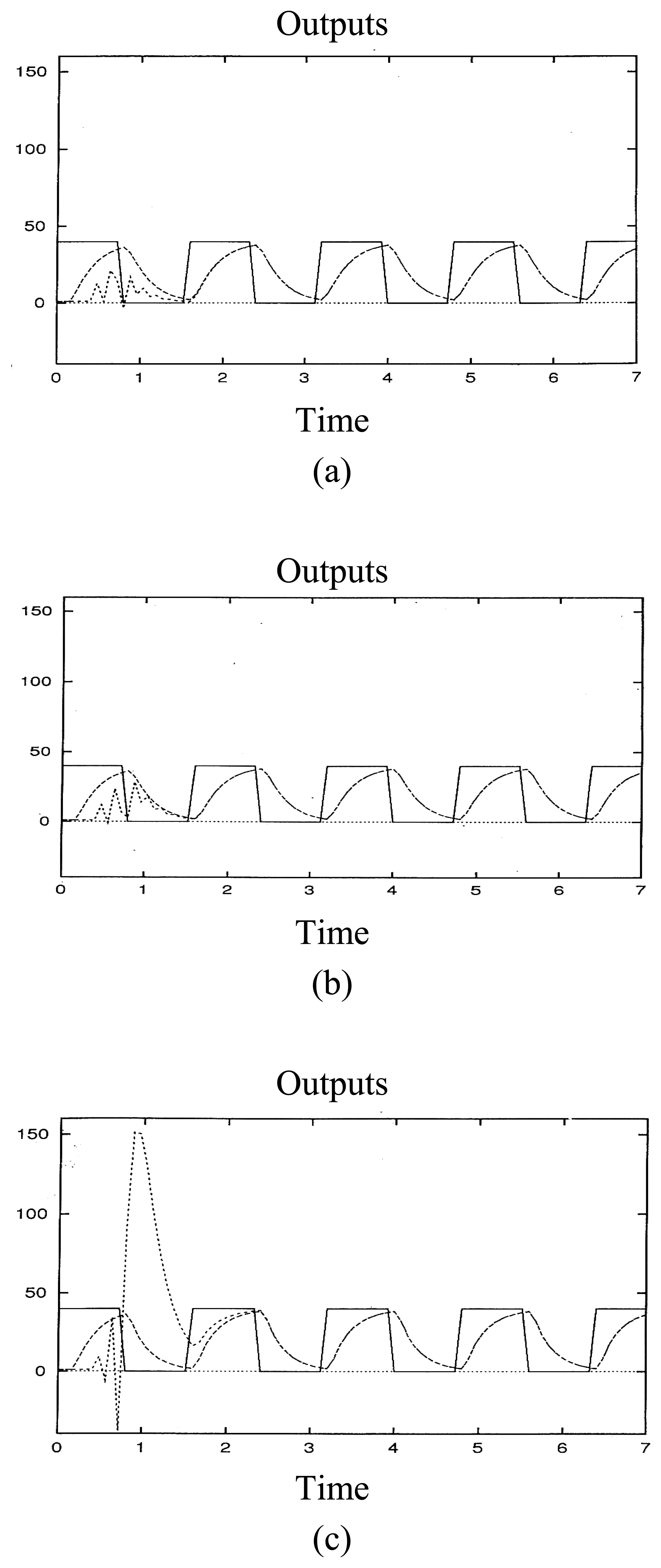
A new example is performed to check the transient performances under different holds and oscillatory inputs. It is assumed that a continuous-time reference model of transfer function G m ( s ) = 60 s 2 + 19 s + 60 specifies the suited performance. The controlled plant is given by the transfer function G ( s ) = 20 2 19.9 s + 60 of parameters assumed to be unknown. Both plant and reference model are discretized under different holds of gains β=0 (ZOH), β=0.2 and β=1 (FOH) resulting in the respective discrete transfer functions H (z) and H β (z) which incorporate the sampling and hold devices in cascade with the corresponding continuous transfer functions. Then, a model-matching based discrete adaptive controller is used which consists of a discrete precompensator and a discrete feedback compensator which are used to generate the plant input at sampling instants. Both compensators are designed such that the closed-loop system transfer function matches that of the reference model. The input to the continuous plant during the inter-sample intervals is generated according to the reconstruction laws of discretized signals under, in general, fractional sampling and hold devices. The initial covariance matrix of the least-squares adaptation algorithm is diagonal with all the diagonal entries being identical to 105. All the initial estimated parameters are fixed to unity, the sampling period is taken to be T= 0.08 secs. and the initial conditions of the plant and reference model are assumed to be zero so that only the forced responses are evaluated. The reference input to the reference model is a almost square nonnegative signal. Such a signal is appropriate to check transients because of its fast changing shape. The resulting control scheme is displayed in Figure 3.
The closed-loop plant outputs for the three tested sampling and hold devices are displayed in Figures 4 together with the reference signal injected to the reference model. Note that there is an asymptotic tracking of the reference output by the plant output as expected with a negligible inter-sample ripple deviations, related to their maximum values, for the three sampling and hold devices tested as expected. However, the three behaviors are quite distinct during the adaptation transients. The fractional order-hold with β=0.2 exhibits the better performance transient behavior, the first-order-hold exhibits the worst one and the ZOH exhibits an intermediate tracking performance.

Acknowledgments

The author is very grateful to The Spanish Ministry of Education by its support through Grant DPI 2006-00714 and to the Basque Government by its support through Grants Research Groups No. 269 and SAIOTEK 2006: S-PED06UN10. He is also grateful to the referees by their useful comments.

References and Notes

  1. De la Sen, M. A method for general design of positive real functions. IEEE Transactions on Circuits and Systems I: Fundamental Theory and Applications 1998, 45(7), 764–769. [Google Scholar]
  2. De la Sen, M. Relationships between positive realness of continuous transfer functions and their digital counterparts. Electronics Letters 1999, 35(16), 1298–1299. [Google Scholar]
  3. Liang, S.; Ishitobi, M.; Zhu, Q. Improvement of stability of zeros in discrete multivariable systems using fractional-order-hold. International Journal of Control 2003, 76(17), 1699–1711. [Google Scholar]
  4. Liang, S.; Ishitobi, M. The stability properties of the zeros of sampled models for time-delay systems in fractional order-hold case. Dynamics of Continuous, Discrete and Impulsive Systems – Series B- Applications & Algorithms 2004, 11(3), 299–312. [Google Scholar]
  5. Miskowicz, M. Asymptotic effectiveness of the event-based sampling according to the integral criterion. Sensors 2007, 7(1), 16–37. [Google Scholar]
  6. Suh, Y.S. Send-on-delta sensor data transmission with a linear predictor. Sensors 2007, 7(4), 537–547. [Google Scholar]
  7. Suh, Y.S.; Nguyen, V.H.; Ro, Y.S. Modified Kalman filter for networked monitoring systems employing a send-on-delta method. Automatica 2007, 43(2), 332–338. [Google Scholar]
  8. Burge, S.R.; Hoffman, D.A.; Hartman, M.J.; Venedam, R.J. Automated ground-water sampling and analysis of hexavalent chromium using a “universal” sampling/analytical system. Sensors 2005, 5, 38–50. [Google Scholar]
  9. De la Sen, M. On the properties of reachability, observability, controllability and constructibility of discrete-time positive time-invariant linear systems with aperiodic choice of the sampling instants; Discrete Dynamics in Nature and Society, 2007; Article ID 84913; pp. 1–23. [Google Scholar]
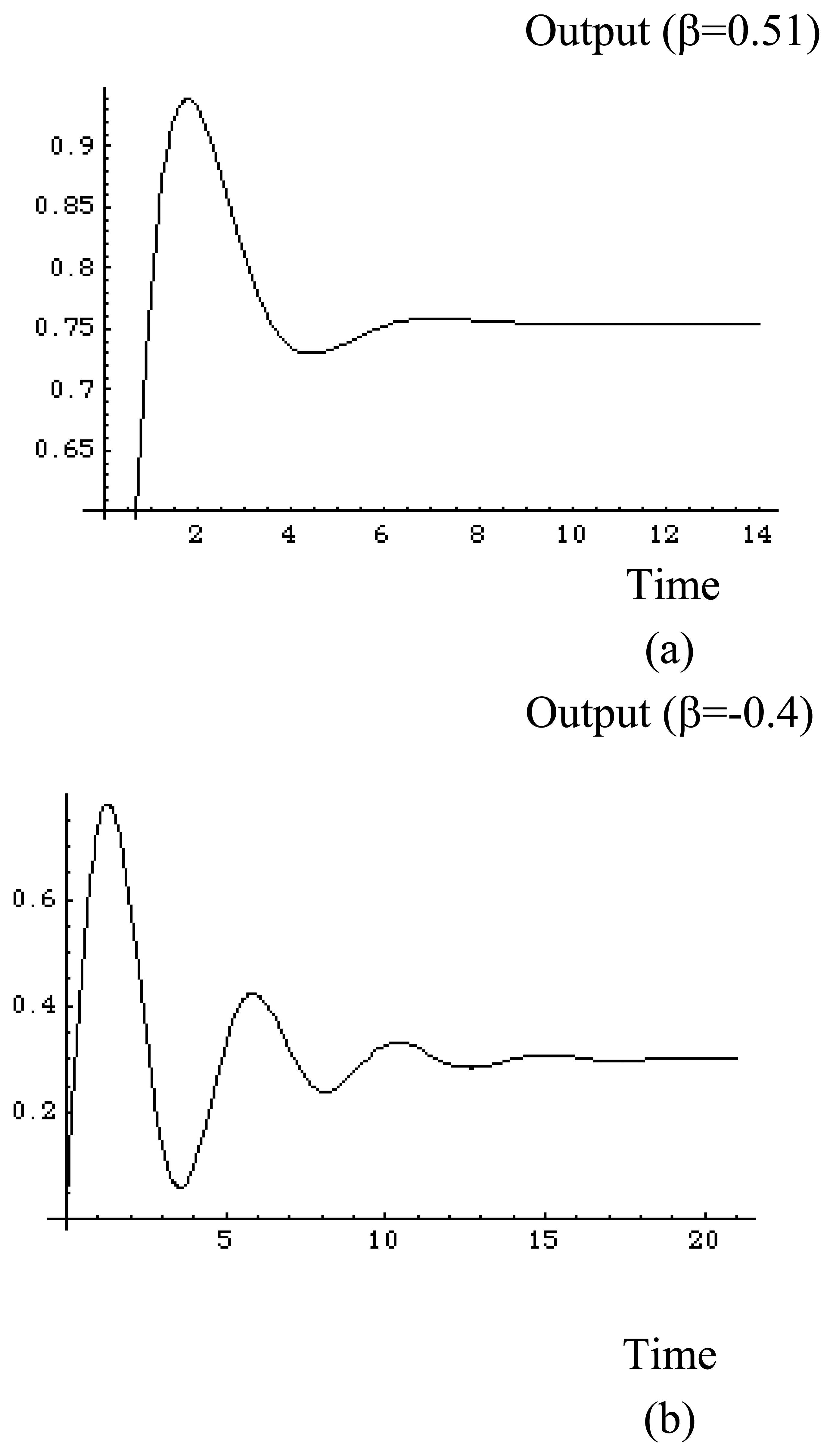
Figure 1. Output inter-sample performance: (a) β=0.51, (b) β=-0.4.
Sensors 07 03146f1
Figure 2. Loss values for β ranging within [−1,1].
Sensors 07 03146f2
Figure 3. Control scheme.
Sensors 07 03146f3
Figures 4. Adaptive transient performances: (a) β=0, (b) β=0.2, (c) β=1; ─ Reference model input, ------ Reference model output, …… Plant output.
Sensors 07 03146f4
Table 1. Loss performances versus values of the correcting gain β
β= 0(ZOH)-0.20.460.471 (FOH)
Loss (Eq. 9)= 16.60925.916541.8494.53180.282

β= -0.25-0.26-0.28-0.30-0.33-0.34-0. 38-0.40-0.5-1
Loss (Eq. 9)= 26.2826.9626.9621.9233914.0767.77302.07791.925.991673.32083