Abstract
The main limitations of standard nadir-looking radar altimeters have been known for long. They include the lack of coverage (intertrack distance of typically 150 km for the T/P / Jason tandem), and the spatial resolution (typically 2 km for T/P and Jason), expected to be a limiting factor for the determination of mesoscale phenomena in deep ocean. In this context, various solutions using off-nadir radar interferometry have been proposed by Rodriguez and al to give an answer to oceanographic mission objectives. This paper addresses the performances study of this new generation of instruments, and dedicated mission. A first approach is based on the Wide-Swath Ocean Altimeter (WSOA) intended to be implemented onboard Jason-2 in 2004 but now abandoned. Every error domain has been checked: the physics of the measurement, its geometry, the impact of the platform and external errors like the tropospheric and ionospheric delays. We have especially shown the strong need to move to a sun-synchronous orbit and the non-negligible impact of propagation media errors in the swath, reaching a few centimetres in the worst case. Some changes in the parameters of the instrument have also been discussed to improve the overall error budget. The outcomes have led to the definition and the optimization of such an instrument and its dedicated mission.
1. Introduction
Topex/Poseidon, Jason and Envisat are currently orbiting, delivering data for ocean monitoring and forecasting. Addition of spatial radar altimetry observations to in-situ measurements and models has given evidence of success for the last decades (see [3]). However, a limit has been reached that nadir altimetry cannot overcome without launching several radars at the same time. The two main drawbacks of nadir altimetry are lack of spatial and temporal coverage and a limited observed swath (typically 2 km for T/P and Jason). Ocean mesoscale phenomena with spatial scales that can go down to a few tens of kilometres and amplitudes in the range of 50 centimetres play a major role in the ocean dynamics: they remain largely undersampled.
A new and revolutionary altimetric measurement has been assessed for the past few years (see [1, 2]). Indeed, mixing altimetry and interferometry, it increases by almost a hundred times the observation swath and aims at keeping a typical measurement error budget of about a few centimetres to catch most of the ocean circulation (see [3] and [4]). The Wide Swath Ocean Altimeter (WSOA) was originally expected to be implemented onboard the Jason-2 satellite in 2004, but the WSOA is not now going ahead (WSOA main parameters are recalled in the table of Figure 24). A global study of the performances of this instrument and its interactions with any external factors was driven by CNES (Centre National d'Etudes Spatiales) in cooperation with NASA/JPL (Jet Propulsion Laboratory) since the end of 2003. Every error domain has been checked and the outcomes have led to the definition of a dedicated mission to such an instrument.
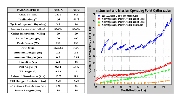
Figure 24.
New operating characteristics for improving the height budget.
In the first section, we give an overview of the geometric layout of such concepts mixing altimetry and interferometry. We assess the derivation of the observed target features (position and height). Subsequently, based on the physics of the interferometric measurement for a given configuration (frequency, chirp bandwidth, antenna length, interferometric base, etc.), we set-up the instrumental error budgets leading to the performance estimation. Instrumental height error profiles are finally simulated for several processing configurations. The above-mentioned approach is primarily applied to the nominal profile of the WSOA onboard Jason-2.
In the second section, the impact of external error sources is evaluated: platform (attitude, atmospheric drag), and propagation media (ionospheric and tropospheric effects). Subsequently, we focus on the required quality of a specific ground processing procedure dedicated to the roll angle determination, which is shown to be a critical aspect of the concept.
A data simulation case is presented in the third section. It is based on real data acquired during the tsunami episode of December 26th, 2004. Some of the possibilities offered by such concepts are illustrated.
Finally, the last section develops a new set of instrument characteristics and dedicated mission by taking into consideration the outcomes of the previous error budget studies. An overall satellite configuration (platform + payload) is proposed, which optimizes the existing technologies in order to much better answer the scientific objectives.
2. Instrument operating characteristics
Before going into some details in the technique of wide swath interferometric altimetry and into the optimization of a proposed space mission to primarily observe ocean mesoscale features, let us recall one main requirement at mission level. Indeed, to observe ocean mesoscale features and assimilate observations in models usefully, it is now agreed that the lower the nadir altimeter instrument range noise, the better mesoscale features will be retrieved, assuming that resolution is provided thanks to multiple orbiting instruments in a well-phased configuration. The optimal range noise level is at the level of some 2 cm, which is a figure that is reached by the well known TOPEX, POSEIDON-1, POSEIDON-2, ENVISAT RA-2 instruments in typical situations characterized by a 2 meter significant waveheight and a 11 dB backscatter coefficient. As far as swath instruments are considered, estimating the measurement noise is a multi-parameter task that will be described in the coming sections. For the purpose of data assimilation in ocean models, it is important to have a good knowledge of the statistics of the error measurements over the entire swath. Previous use of wide-swath simulated data in a high-resolution ocean model have shown that a 4 to 5 cm overall noise level may be adequate to retrieve ocean signals at the same level as would be achieved by a constellation of 3 to 4 nadir instruments (see [4]). Thus, the basic assumption of the paper will be to design an instrument and a complete system to reach such a 4 to 5 cm noise level.
2.1. Geometry of the system
Both swaths are the results of an off-nadir observation by two passive antennas separated by a mast (see Figure 1 (a)). Compared to conventional SAR interferometry (see [5]), look angles are kept small to get a good level of return power while getting the widest swath possible. The optimal working mode consists in transmitting from one given antenna once every two pulses, while the reception is made by both antennas, to permit further interferometric processing (see Figure 1 (a)). The electronics remains on the central payload to prevent propagation losses all along the interferometric baseline. Then both antennas are tilted by 45 degrees from the mast and double polarization feeds enable both swaths to observe and distinguish signal returns (see Figure 1 (b)).
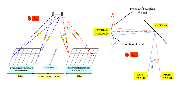
Figure 1.
(a) Lay-out of the geometry of observation (b) Antenna and feeds configuration arbitrarily for the right swath; on the other side, feeds' polar are reversed (Emission/Reception H Feed and Reception. V Feed); a V-polarization pulse is emitted by one antenna, and the consecutive pulse, with H-polarization, is emitted by the second antenna; both polarizations are received by the two antennas.
The purpose of this subsection is to figure out how the real height and position of an observed target within one given swath is derived from the collected data. The determination of the altimetric measurement requires the precise knowledge of four main parameters: the altitude H given by the POD (Precise Orbit Determination), the range r1 from the master antenna to one pixel coming from the onboard clock, the roll angle α and the interferometric phase Φ, calculated onboard. The roll angle, whose a priori knowledge is given by the PAD (Precise Attitude Determination), happens to be a critical parameter and has then to be accounted for. A dedicated calibration process using crossover data will also have to be implemented to reach optimal performances.
As illustrated on Figure 2 (a), let us consider a target inside the right hand-side swath. For pulses of wavenumber k, the parameters quoted previously enable us to calculate the height h above the plane tangential to the surface at nadir:
and its position X as:
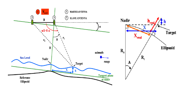
Figure 2.
(a) Geometry of the interferometric measurement (b) Local Frame Transformation.
The height measurement h and the exact position of the target X inside the swath, primarily referenced against the tangent plane and reference altitude at nadir, are more conveniently expressed in a local frame: hreal and Xreal (see Figure 2 (b)).
POD performances directly impact the knowledge of r1 and then hreal. The precise knowledge of the roll angle comes from the PAD and from a post processing procedure using crossovers estimation (see Section II.3). Last but not least, the quality of the onboard estimation of the interferometric phase is primitive and needs to be further investigated. It should be noted that the phase unwrapping process is not a critical point in our configuration (unlike standard SAR interferometry applications). Indeed, the altitude of ambiguity (see [6]) ranges from 25 m at the NR (Near Range) to 170 m at the FR (Far Range), which is much larger than the few tens of centimeters magnitude of expected observed phenomena.
2.2. Interferometric phase
The interferometric phase measurement quality is strongly related to the coherence value γT between the two receiving channels. This coherence is mainly affected by three factors: the instrument signal to noise ratio, the range migration within the swath, and the speckle (its effect is also called geometric decorrelation (see [7]). An onboard process enables to correct the impact of speckle effect (see [1, 2]). Furthermore, accounting for the very small range of incidence angles (less than 5°), the second term becomes negligible compared to the first term, directly related to the instrument features. Therefore the coherence between signals is mainly driven by the SNR:
The interferometric phase statistics are distributed according to the Wishart distribution (see [8]), depending on the number of looks and the coherence between the two received signals. Assuming both signals have complex circular Gaussian distributions, the computation of the argument of their product of correlation leads to the following probability density function of the interferometric phase (see [9-13]):
where Γ(.) is the Gamma function and F(.) the hypergeometric function (see [14]).
Figure 3 (a) illustrates the dependence of the pdf on coherence γT for a single look and Figure 3 (b) illustrates its dependence on the number of looks for a typical correlation of 0.9 (see next subsection). These plots show that the instrument parameters (related to the SNR) must be selected to guarantee the highest possible degree of coherence to avoid the need for extensive multi-look processing, which would result in poorer intrinsic spatial resolution.
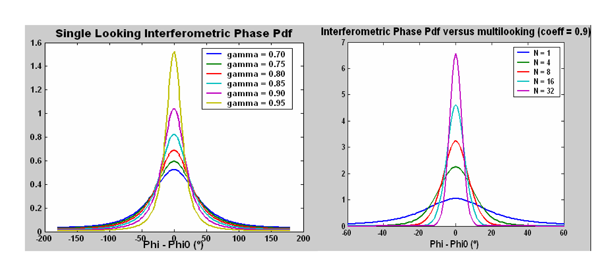
Figure 3.
Interferometric phase densities of probability versus coherence (a) and multi looking (b).
The phase variance can be numerically calculated from (6); above a certain number of looks, it can be shown that it can be well approximated by the Cramer-Rao bound (see [15]), in the case of high coherence values (see Figure 4):
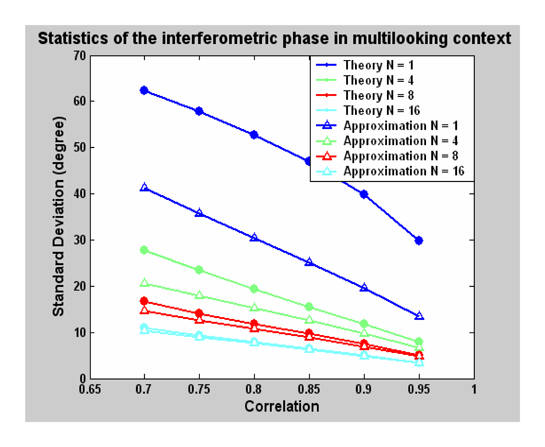
Figure 4.
Statistics of the interferometric phase in multilooking context.
This approximation strengthens the need for a large degree of coherence. The next subsection will confirm this behaviour when entering the details of the WSOA operating characteristics.
Therefore, the instrument SNR has to be studied carefully, as the main contributor to the decorrelation between the two channels. The analysis of the derived degree of coherence in the swath will then fix the multilooking strategy to be implemented. Indeed, the objective of such a strategy will be to reach the desired standard deviation of the estimated interferometric phase that keeps the height performances within the range of constraints specified by the targeted scientific objectives.
2.3. Instrument performance: SNR and Height Error
The signal to noise ratio for an extended target (a resolution cell) can be expressed as follows, where the different terms refer respectively to the range loss, the EIRP (Equivalent Isotropic Radiated Power), the effective antenna surface, the range resolution, the azimuth resolution, a global addition of different losses related to the instrument RF and the atmosphere, the reception channel noise, the range compression gain and the observed scene contribution through the backscattering coefficient (see [16-19]):
Based on published specifications for WSOA ([1, 2]), the derived coherence of the received signals is plotted in Figure 5 (a). Values are larger than 0.9 for more than 90 % of the swath (Note than the centre of the swath benefits from a coherence value close to 0.97; the bell shape stems from an optimization processing described in the following). The performances of the instrument are related to the onboard interferometric phase estimation that is related to the SNR and the desired geometry of the final pixel; the equation providing the expression of the height error can be written as:
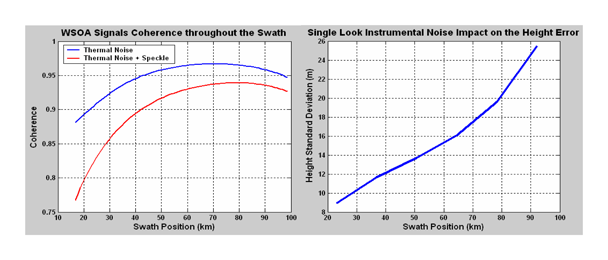
Figure 5.
(a) WSOA signal coherence throughout the swath with and without the onboard correction of the geometric decorrelation (b) Single looking instrumental noise impact on the height budget.
Figure 5 (b) shows the height errors (expressed in meters) related to a single looking process, that is to say a resolution cell of 13.5*0.6 km in the NR to 13.5*0.1 km in the FR (assuming an orbit height of 1334 km and the antenna beamwidth in the along track direction to be around 0.55°). The 10 to 25 m order of magnitude is considerably greater than the scientific objectives (4 to 5 centimeters). Even with a stronger coherence, performances would remain very poor. Therefore we cannot avoid an extensive multilooking process. The size of the onboard post-processed pixels has then to be determined to comply with the following conditions: (i) keep it as small as possible to allow additional ground processing procedures to be used for extra averaging in order to lower noise if needed, (ii) make this size large enough to allow for the feasibility of data downloading to Earth terminals, given affordable telemetry rates on usual satellite platforms. Let us also add that because the complex onboard process is irreversible, a small pixel size would be preferable to avoid losing any information from the raw observations.
Figure 6 displays a plot of the number of looks and the standard deviation of the height error as a function of the pixel position in the swath. Four pixel dimensions have been tested in the range direction whereas a fixed 16 km scale (corresponding to 13.5 km plus distance moved in 400ms) is imposed in the azimuth direction. A 1030.05 Hz PRF per antenna is considered. Looks are counted with regard to the onboard incoherent averaging procedures. Ground segment algorithms may adopt an increased number of looks in order to improve the resulting performances: however, ground algorithms are beyond the scope of this performances study.
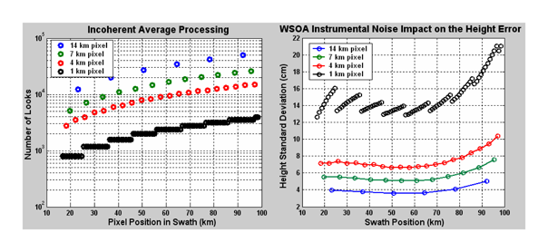
Figure 6.
(a) Number of looks associated with different incoherent average processing procedures in the range direction (b) Associated WSOA instrumental noise impact on the height error (the digitization step in the number of looks is related to the intrinsic range resolution, that results in discontinuity when considering 1 km pixels).
The 4 to 5 cm objective can be reached when the averaging process is applied over 16*14 km pixels (see Figure 6 (b)). If finer data are required, e.g. with 1 km resolution in the range direction, noise is increased by almost a factor of 4. The strategy for WSOA as a Jason-2 instrument was to retrieve the interferometric phase over 16*1 km pixels on-board, before data downloading. In this case, the possibility of applying the multi-looking process on ground offered a key degree of freedom.
Another major objective is to get a quality of measurement as uniform as possible over the swath. However, degradations caused mainly by the range loss, the backscattering coefficient and the range resolution are far more important at the edge of the swath. The center of the antenna beam has then to be oriented toward the far range of the swath in order to maximize the gain there and compensate these losses. Figure 7 shows that a 3.5 degree antenna boresight produces an almost flat height standard deviation across the whole swath. This optimization results in the coherence previously shown in Figure 5 (a).
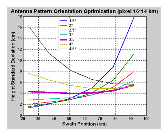
Figure 7.
Antenna Pattern Orientation Optimization.
The required instrumental error is so stringent that a large amount of multilooking is necessary. There is a modification that could be brought to the WSOA operating characteristics that could help get slightly better coherence, and allow us to reduce the number of looks and thus improve the intrinsic spatial resolution (see section 5).
However, the WSOA operating characteristics cannot be completely assessed and discussed without determining the impacts of external factors on the error budget. This is the purpose of the next section.
3. Impact of external errors
Only instrumental effects on the error budget have been reported yet. External effects need to be analysed and associated errors shall then be incorporated in the overall budget. The ones stemming from the errors on the POD and the radiometer measurement as well as the electromagnetic bias are already well known thanks to current missions. Their in-depth study is not the purpose of this section.
First of all, we will focus on the influence of the platform attitude. Two components of the three dimensional attitude angles are considered. On the one hand, yaw rotation is considered: indeed, as selected orbits can be sun-synchronous or not, the use of a yaw motion may be required to supply energy to the carrier satellite. It will be shown that a yaw rotation significantly degrades the spatial coverage; on the other hand, the impact of a roll motion is estimated, and will be shown to hugely amplify the height error.
Last, electromagnetic wave propagation perturbations through the ionosphere and the troposphere will be statistically reviewed. We will consider worst case scenarios as is usual when evaluating instrument performances and dimensioning systems.
3.1. Impact of orbit selection
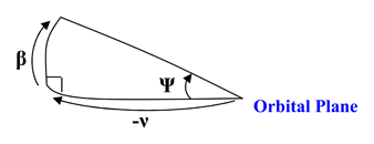
The Jason-2 orbit, as the ones from Topex/Poseidon and Jason, has been constrained to be non sun-synchronous to cope with the tidal aliasing. However, this kind of orbit requires a strong attitude control onboard so as to keep the solar panels directed toward the Sun, by driving the yaw angle rotation around the axis directed toward the Earth, called yaw steering (see Appendix A). The most constraining angle to look at is the angle between the Sun and its projection on the orbital plane, called β angle; for a repetitive orbit, this angle has strong variations and goes null 6 times per year, corresponding to the best position of the Sun in the orbital plane. It impacts directly the yaw angle and then the geometry of the swath. The width of the swath at a given yaw can be expressed as followed:
where
where L0 is the nominal width in the range direction, Raz the azimuth resolution, Ψ the yaw angle and ν the angle between Earth-Sun vector projection on the orbital plane and Earth-Satellite vector.
Figure 8 (a) illustrates both the yaw and beta angle evolution onboard the Jason-2 platform over an entire year. The six best periods are 12 days long (green circles in Figure 8). They correspond to no yaw steering when the Sun is within 15° of the orbital plane.
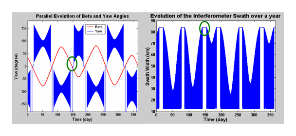
Figure 8.
(a) Yaw steering onboard Jason-2 over a year (b) WSOA Swath Width over a year. Note the yaw and swath width vary between the minimum and maximum of their envelope within each orbital period.
Figure 9 (a) illustrates the daily evolution of the yaw angle versus the latitude. The yaw angle evolves almost periodically with the orbit; it covers a very wide range of values when a steering motion is on, varying in the +/- 90° range twice an orbit; in the worst case, the width of the swath reaches a minimum which corresponds to the azimuth resolution of the instrument. The geographical distribution of the swath width is symmetric with respect to the equator: the minimal width area moves from the equator to the poles when β goes from +/-15° to +/- 90°. When β is close to the maximum, the yaw angle remains close to +/- 90° and the width of the swath is always of the order of a few tens of kilometres only (see Figure 9 (b)).
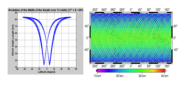
Figure 9.
(a) Evolution of the Swath over 13 orbits at the beginning of yaw steering (b) Width of the swath over 10 days in the worst case (-75°<β<-73°).
Furthermore, these rotated configurations of the resolution cells deteriorate the averaging process and the formation of clean final pixels. If we only consider valid data at zero yaw angle, the global functioning time reduces to 20 % of the overall mission lifetime (see Figure 10 (a)). The Doppler centroid, that is the weighted mean of the Doppler shifts within a look direction, is given by Equation (12) and Figure 10 (b)), As this is not corrected onboard, it has to be taken into consideration in the ground processing algorithms. Besides, the efficiency of the correction imposes an intrinsic range resolution as short as possible.
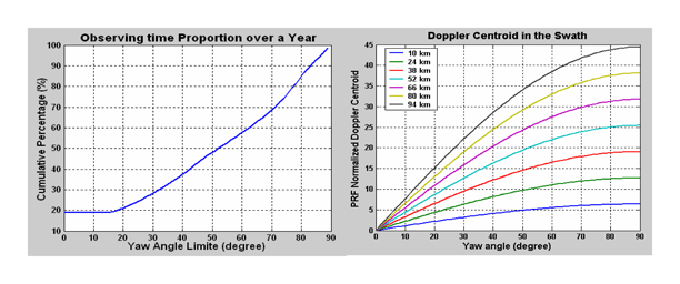
Figure 10.
(a) Impact of the yaw steering onboard Jason-2 on the predicted observing time (b) Impact on the signal processing in terms of Doppler centroid.
Finally, this orbital configuration leads to the orientation of the solar panels perpendicular to the satellite velocity. The atmospheric drag has known effects causing the semi major axis to drift and then the ground track to move, as follows (see [20], all variables are defined in Appendix 2):
Sticking to classical repeat orbits that remain located within a +/- 1 km band from a nominal ground-track (to make easier the study of time-varying phenomena), we can then infer the frequency of maneuvers to maintain the orbit as it is required.
The required rotation of the panels around their symmetric axis extends the surface drag of the satellite, accelerating the frequency of maneuvers and then reducing the satellite life-time or degrading the mass and cost budgets. In addition, the rotation of the interferometer antennas around the yaw axis further increases the drag.
Figure 11 shows how the atmospheric drag can be decreased by approximately 80 % when selecting a sun-synchronous orbit. As a consequence, the frequency of maneuvers – which can be calculated from Equation (14) (see Appendix 2) that gives the duration between 2 successive maneuver s- is decreased by a factor of 5.
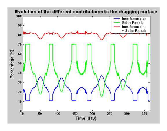
Figure 11.
Evolution of the different contributions to the overall satellite surface drag.
As far as the interferometric altimetry system is considered, flying a sun-synchronous orbit would eliminate many of the drawbacks of flying a non sun-synchronous one: (i) the observation geometry would be kept constant, (ii) the carrier platform could be made very stable and the sun-satellite relative geometry would be always optimal to provide energy to the satellite, avoiding negative impacts on the interferometric error budget. The overall impact of this change of orbit, and especially the problem of tidal aliasing will be considered in section 5.
3.2. Impact of environmental effects
The range value between the target in the swath and the master antenna r1 is used during the ground altimetric process (see I.1). This range is affected by several sources, principally the ionospheric and tropospheric delays.
3.2.1. Ionosphere
The ionospheric delay is mainly dependent of the Total Electronic Content (TEC) and the radar signal frequency. The nadir altimeter, which now commonly operates at two frequencies, has thus the ability to determine the TEC along its path and in the mean time the ionospheric delay. However, this measurement only applies in the nadir direction, and not in the off-nadir direction. Therefore, there is an error in applying the nadir ionospheric delay to the interferometer master antenna range.
The ionosphere is known to have variability with spatial wavelengths of the order of one thousand kilometers. However, in order to get an accurate error budget, the maximum amplitude of TEC variations over about 100 km (FR) must be determined (worst cases consideration). Dual-frequency ionospheric data have already been computed along nadir altimeter paths (see [4]). They only enable us to determine these ionospheric delays along one direction. However, delays must also be known along the crosstrack direction and even along all directions because of the yaw steering. GIM (Global Ionospheric Model) maps resulting from GPS (Global Positioning Satellites) worldwide data are available daily and have been intensively validated (see [21, 22]). They constitute the best dataset to derive global statistics of the worst cases. Figure 12 shows an example of the errors for April 2000, plus a summary of the results for the years 2001 and 2002.
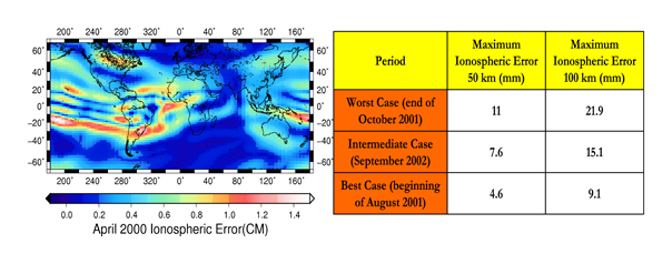
Figure 12.
(a) Example of the spatial distribution of the FR ionospheric errors (differences between the nadir and the off-nadir delays) in an intermediate case at midnight in April 2000 (b) Maximum ionospheric errors in the swath (Middle Range and Far Range) in different cases.
Statistics show that ionospheric errors (difference between the nadir and off-nadir delays) above 0.7 cm in the Middle Range (MR) and 1 cm in the Far Range (FR) are common, especially in the tropics. Then, the use of worldwide GPS data in the ground processing segment can be an appropriate solution to solve such an issue.
3.2.2. Wet troposphere
The case is similar for the tropospheric correction, which is derived from measurements of a three-frequency nadir radiometer (18.7, 23.8 and 34.0 GHz) that is a standard part of an optimal altimetry payload. The amplitude of the variations of the water vapor content of the troposphere have been looked at through the computation of SSMI (Special Sensor Microwave Imager) data (see [23]), the worst cases being analyzed during periods of Hurricane Juan in fall 2003. First of all, the overall mean error (difference between the nadir and the off-nadir wet tropospheric delays) in the FR has been analyzed versus latitude. Stronger signals in the tropics result in an error that may be 50 % larger than the global average (see Figure 13 (a)). Maximum errors can reach 3 cm in the Middle Range (MR) and beyond (see Figure 13 (b)). Occurrence of the Hurricane Juan on the 30th of September is clearly visible in the tropospheric error plots (see arrows).
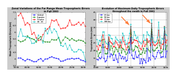
Figure 13.
(a) Zonal variations of the Far Range mean tropospheric error in October 2003 (b) Worst cases tropospheric errors during fall 2003 with evidences of the Hurricane Juan (orange arrows).
The statistical distribution of the errors when going through a typical large atmospheric feature (a few hundred of kilometers wide) has been computed (see Figure 14 (a) and (b)). For distances within the swath larger than 50 km, almost 50 % of the errors go above 1 cm.
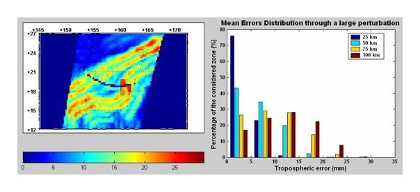
Figure 14.
(a) Spatial differences in wet tropospheric delays over a large atmospheric feature (typically a few hundred kilometers wide) in mm (b) Statistical distributions of the tropospheric errors over the feature.
3.3. Impact of roll angle knowledge
The roll angle plays a major role in the height estimation process (see I.1): a roll error linearly impacts the height measurement thanks to the across track distance in the swath x according to:
Applying Equation 15, a one arc second error in the knowledge of the roll angle results in a Far Range height error about 50 cm. It then comes that a 0.1 arcsecond maximum error is acceptable, given the 5 cm requirement corresponding to the overall error budget of the height parameter.
An a priori knowledge of the roll angle spectral characteristics is provided by the PAD system onboard the satellite. However, the required accuracy of less than a tenth of an arc second is so strong that ground post processing procedures using crossover data need to be done. A crossover is an area where an ascending track crosses a descending track. In the case of WSOA, swath/swath, nadir/swath and nadir/nadir crosses shall be considered as calibration points (see Figure 15). Two successive crossover locations along a track are only 80 seconds apart as a maximum. Thus, assuming we get rid of the high frequency part of the roll spectrum in the PAD, an appropriate interpolation scheme between crossovers may finally give an overall a posteriori knowledge of the roll angle that lies within the specifications.
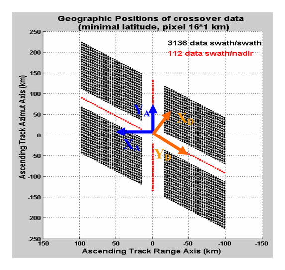
Figure 15.
Geometry of crossovers measurements and definition of the appropriate local frame.
Rodriguez and al ([2]) have computed a crossover maximum likelihood estimation of the roll angle in the WSOA/Jason-2 case, considering a 14 km intrinsic range resolution. The goal of the current study is to determine the influence of external factors on the quality of the roll estimator: the ground pixel size after incoherent onboard processing, the repeat cycle of the orbit and finally the presence of nadir altimeter data.
The main idea of the crossover estimator is that the over flying time of the crossovers zones are small enough to consider a linear evolution of the roll angle with time (see Figure 16 (a)) as followed:
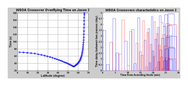
Figure 16.
(a) Latitudinal Dependence of the interval between successive crossovers (b) WSOA Jason-2 crossovers characteristics: blue refers to ascending tracks first and red to descending tracks first; each rectangle corresponds to one crossover, its width defining how long it is over flown.
Four parameters (two for the ascending track, two for the descending track) are then to be estimated:
The height differences at the crossovers are dependent on several factors, which are respectively the roll parameters associated to the geometry of the crossovers (see Figure 15), the instrumental noises (interferometer and nadir altimeter), the ocean variability and the external noises (tropospheric and ionospheric), and can be expressed as followed (all variables are defined in the table of notations):
The interferometer noise and the external noises are derived from previous sections. The nadir altimeter noise is assumed to be 2 cm (see [24]). The covariance of the SLA (Sea Level Anomaly) is computed from [25] as a function of latitude. A maximum time difference of 5 days between ascending and descending tracks has been used in the selection of crossovers to avoid high temporal decorrelation. Thus, for Jason-2, all crossovers can then be considered (see Figure 16 (b)).
“A-D” (ascending minus descending) differences in Equation (18) are the observations, which we will call di, which can be represented using the following:
where m(θ) = Hθ, and (Ni) have covariance matrices R independent of θ. H can be easily expressed in the local frame and (Ni) are related to all the noises defined in Equation (18). Covariance matrices of the estimated parameters can then be computed as followed, leading to the knowledge of the quality of the process:
The quality of the estimation is defined by the standard deviation of the roll angle, related to the residual error in its knowledge (in arcsec).
The histogram in Figure 17 (a) shows that the shorter the repeat cycle, the better the estimation. The main reason is the ocean decorrelation which becomes very important above 5 days (see [25]). The histogram in Figure 17 (b) shows that even a very small number of nadir/swath measurements help decrease the error in the a posteriori knowledge of the roll angle. Finally, the last histogram in Figure 18 shows that the minimum onboard incoherent processing (going to 3 km pixels almost removes errors greater than 0.05 arc second!). Indeed, it would be better to do the estimation with high-resolution data, even if the precision is lower, and then add a ground average processing procedure to get the final pixel resolution more compliant with the required height precision.
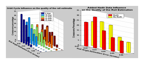
Figure 17.
(a) Influence of the orbit characteristics on the quality of the processing (b) Influence of the presence of nadir altimeter on the quality of the processing.
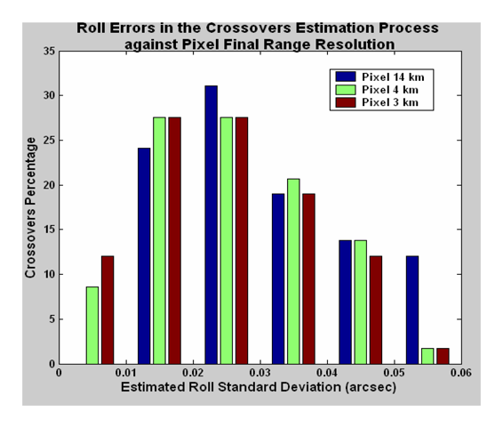
Figure 18.
Influence of the pixel range resolution on the quality of the estimation process.
Processing crossovers may also enable us to correct the linear part of the ionospheric and tropospheric gradients errors in the swath, which would then be assimilated as an additional roll angle.
3.4. Overall WSOA Error Budget
Results from the last two sections eventually will provide an overall performances budget (see Figure 19) of WSOA onboard Jason-2. In order to show the influence of external errors, the 16*14 km post processing pixel was selected. Best and worst cases are mainly dependent on the media propagation and attitude errors. The residual roll error in worst case was taken equal to 0.12 arcsecond (see II.3). POD error is equal to 2.5 cm (Envisat error budget), electromagnetic bias to 2 cm, dry troposphere to 0.7 cm, and nadir radiometer to 1.2 cm (Jason error budget). The error in the determination of the ionospheric delay with the dual frequency nadir altimeter is taken equal to 0.5 cm (see [26]). Finally, the baseline length error comes out from the consideration of a 1 K temperature accuracy and a thermo elastic coefficient of the mast of 10-6.
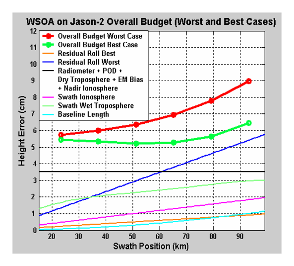
Figure 19.
Global error budget of WSOA in worst and best cases for 16*14 km
On a worst case basis, the contribution of the instrumental error (see Figure 6 (b)) to the global budget is about 55 % for a 16*14 km pixel; if we compute the overall budget over a 16*1 km pixel, the contribution goes up to 90 %. Therefore, even if there is a strong need to improve estimates of external sources of errors, improving the performance of the radar instrument would have an impact on improving the performance of the system for high spatial resolution. Section 5 presents a slightly modified operating characteristics for an instrument such as WSOA in order to strengthen this overall error budget. However, before going into such an analysis, section 4 illustrates the scientific goals of WSOA.
4. Data Simulation
A primary advantage of such a WSOA system is that data are collected in two dimensions, namely along-track and across-track. Then surface gradients and Laplacian can be computed, leading to computations of the geostrophic velocity and vorticity (see [20]). Furthermore, the intrinsic resolution (16*1 km) samples the ocean surface enough to determine the structure of most of the ocean eddies at Rossby radius of deformation scales (see [27]) as well as coastal processes (see [28]).
A way to illustrate the usefulness of such a system has been to simulate the observations that could have been done at the time of an extreme ocean event. The case of the December 2004 tsunami over the Indian Ocean is such an example. Indeed, the Topex/Poseidon (T/P) and Jason satellites flew over the area of interest a few hours after the beginning of the seism. However, the direction of the tsunami, as well as an estimation of its power could not be derived from the acquired data. We simulated observations of such a tsunami assuming that an interferometer is implemented on the two platforms, based on CEA (Comité à l'Energie Atomique) outputs of a tsunami propagation model (which has been well validated using the real T/P and Jason-1 altimeter data).
The tsunami started at 0 h 58 GMT at the top North of Sumatra Island. Jason went over the equator, at 85.7° East longitude 116 minutes later. Finally, Topex/Poseidon went over 7 minutes later, at 84.3° East longitude. For the purpose of the simulation, the SLA (Sea Level Anomaly), referring to the height of the water above the MSS (Mean Sea Surface), have been computed. Simulations were performed with post processing resolution of 16*4 km (21 pixels in each swath), which is the best compromise between quality of the height budget and minimal density of measurements to detect small-scale phenomena.
The simulation takes into account the overall instrumental and external factors studied, with the worst cases in propagation errors and attitude errors.
The direction of the tsunami wave can be easily determined from the height profiles derived from the simulated WSOA data on the Jason platform (see Figure 20 (a) and (b)), thanks to the added knowledge in the range direction perpendicular to the satellite velocity. The roll errors, which are correlated across track and along track, are well corrected, thus even in the worst case the residual errors (from 1cm in the NR to 5 cm in the FR) don't prevent from a very good observation of the amplitude of the phenomenon.
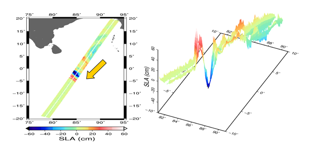
Figure 20.
(a) Simulated sea level anomaly as would have been observed by an interferometer onboard the Jason platform over December 2004 tsunami and determination of the wave direction (yellow arrow) (b) 3D view of the observations (azimuth, range, height).
Figure 21 shows what kind of data a WSOA on Topex/Poseidon would have delivered given the unfavorable yaw angle at the time estimated between 99 and 101 degrees. On the right side of the T/P track, Poseidon 2 track is also plotted. The advantage provided by the large swaths has vanished, and the residual data look like nadir altimeter data..
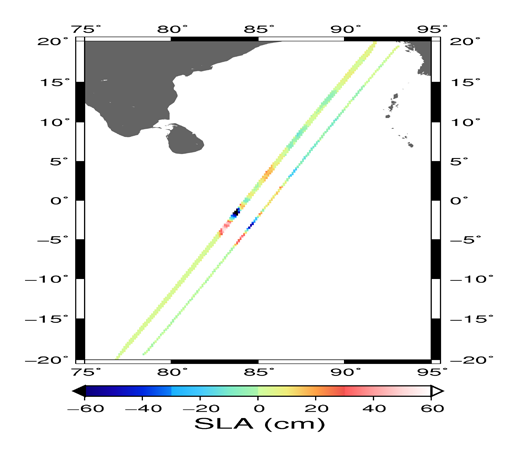
Figure 21.
Simulated interferometer data on T/P platform with yaw steering and Poseidon 2 data to the right of it.
It confirms the strong advantage of getting rid of any platform rotation by moving to a sun synchronous orbit.
5. Overall mission definition and optimization
Let us now assume that the scientific objectives remain the same as for WSOA onboard Jason-2. Some other applications can be considered over coasts and continental basins (typically some tens of square kilometers), but the weak azimuth resolution of several kilometers prevents from studying small scale surfaces. The study of these other potential applications is not the purpose of this paper. They do not provide us with major constraints on the following optimization of the instrument and the dedicated mission. The additional requirement of observing the entire ocean surface between -80 and 80 degrees latitude is brought up. A secondary objective is to maximise the use of technologies that have already been developed, like the mast and the TWTA (Traveling Wave Tube Amplifier).
We focused on areas between 0 and 60 degrees latitude (North and South), as higher latitude areas are well sampled and do not constrain the spatial and temporal coverage. The histogram in Figure 22 (b) confirms the global coverage with less than 1 % unobserved areas (due to the 10 km gaps between nadir and NR). In addition, more than 42 % of the area between -60 and 60 degrees latitude are accessed more than 3 times per cycle.
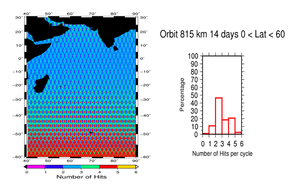
Figure 22.
(a) Number of Hits per cycle of repeatability for a 815 km sun-synchronous orbit over the Indian Ocean (b) Temporal coverage of this orbit between 0 and 60 degrees latitude.
The 9.9156 solar day repeat period of T/P and Jason was chosen to minimize the effects of tidal aliasing (see [29]). One drawback of a 14-day sun-synchronous orbit may lie in the large aliasing periods of the tide harmonics. It may prevent their efficient observation (see Figure 23). However, thanks to T/P and Jason, the major constituents of tides have been mapped with an accuracy better than 2 cm in the deep ocean (see [30]). Shorter wavelengths of the tides may be less well known, but a swath-type observation may provide new insights into the retrieval of small-scale coastal waves (see [31]).
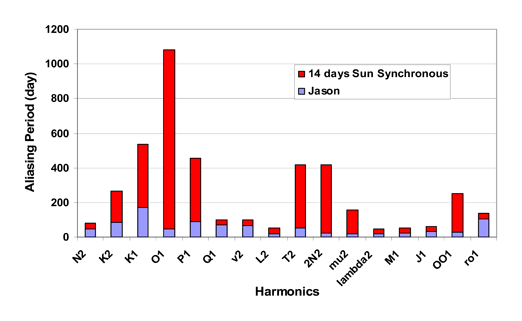
Figure 23.
Tidal aliasing comparison between Jason and the proposed sun synchronous 14-day cycle.
For a given interferometric phase uncertainty, the height error is proportional to the wavelength and to the inverse of the interferometric baseline (see Equation (9)). Ka-band could have been considered as a new carrier frequency since it increases the effective baseline by almost a factor of 3. However, because the maximum peak power out of the amplifiers is proportional to the square of the wavelength to first order, selecting the Ka band instead of the Ku band may lead to technological difficulties in terms of power amplification. In addition backscattering coefficients at Ka-band for small view angles have not yet been fully assessed, even though known tower experiments were run using Ka band instruments. New complex and expensive developments of the TWTA and the antenna reflectarrays would be required that are not worth the performance gain. Therefore Ku band remains the right choice as the carrier frequency, also considering that Ku band backscattering coefficients are very well known given all instruments already using this band to perform radar measurements (see [17] and [18]). The baseline length was limited on Jason-2 because of the size of the spacecraft. Returning to a sun-synchronous orbit releases this constraint. The 10 m specified mast length limit imposed by the manufacturer can then be adopted.
From an ionospheric perspective, the presence of a dual-frequency nadir altimeter onboard the platform is required as the interferometer uses signals whose carrier frequency is in Ku Band or below. Indeed, it is the only way to very accurately cope with the ionospheric correction. However, section II.2.a showed that the interferometer ground processing procedures could take benefit from the use of GPS data in some specific areas in order to extend the correction throughout the swath.
A three-frequency radiometer is of course required; however, using external data such as SSMI or numerical weather prediction analysis to improve the wet tropospheric correction may be considered, especially at low latitudes and in the middle of large storms where the errors can reach more than 2 cm more than 20 % of the time (see Section II.2.b).
The only interest in enlarging the chirp bandwidth would be to get a better resolution in the range direction, which would cost a lot in terms of link budget (leading to degraded performances), power budget and telemetry budget (see [32]). Furthermore, if we limit the mission objectives to oceanographic, coastal and large rivers and basins applications, the current resolution offered by a 20 MHz bandwidth is adequate. Furthermore, the size of the final pixel is in any case mainly constrained in the azimuth direction by the RAR (Real Aperture Radar) resolution around 8.4 km, related to the length of the antennas (see Figure 24).
Conversely, the pulse length should be further checked. It was constrained on Jason-2 by the presence of the nadir altimeter and the telemetry budget. Keeping the nadir altimeter in the new proposed mission freezes the PRF and then constrains the pulse length as well. However, the telemetry budget can be improved and therefore frees a degree of freedom on the pulse length (see [32]). The 120 W TWTA designed onboard Jason-2 has specifications enabling it to function with a maximum duty cycle of 27 %. Chronogram and power budget constraints lead to the selection of a pulse length of a hundred microseconds.
As it was done in Section 3.4, the worst cases external errors are brought up in the overall height budget related to the instrument operating characteristics, which can then be compared to the one on Jason-2 (see Figure 24).
By changing the instrument operating characteristics and the dedicated mission parameters, performances equivalent to a WSOA on a 16*14 km pixel are now likely to be obtained on 12*1 km pixel. The decreasing of the intrinsic surface area has been done by almost 95 %. This huge profit enables to get more hits to phenomena at Rossby radius of deformation scales. Furthermore, coastal observations are improved in the worst case of a perpendicular approach as now the limit distance is no more than 8.4 km. Finally, the 4-5 cm noise level specified in section I is almost reached throughout the whole swath for a 12*4 km pixel; FR data errors fill the constraint when averaging up to 6 km in the range direction (keeping 12 km in azimuth) or up to 13 km in the azimuth (keeping 1 km in range).
6. Conclusion
Wide Swath Altimeters must be part of the future of the overall altimetry observation system. They enable us to get a global coverage of the Earth between -80 and 80 degrees of latitude and an appropriate temporal sampling, required to observe mesoscale phenomena and improve ocean monitoring and forecasting to an unprecedented level. Though their error budget is greater than for a nadir altimeter, and the errors are partially correlated across-track, these new altimeters are the only ones capable of providing us with a global two-dimensional topography of the ocean. Unfortunately, the demonstration of such revolutionary systems could not be incorporated as part of the Jason-2 program. However, studies of such instruments have continued (see [33] and [34]) and hopefully one of them will fly over the oceans to demonstrate their capabilities and add to the scope of nadir altimeter missions.
The studies performed and presented throughout this paper have led to a better knowledge of the performances of this interferometer and its interactions with all kinds of external factors, finally enabling us to optimize the instrument parameters as well as the definition of the overall mission. Different levels of accuracy associated with different pixel resolutions can be achieved. In addition, integrating overlapping passes over the whole mission lifetime will enable to get even better accuracy.
Acknowledgments
There have been a number of people whose assistance has made this research possible. V. Enjolras especially likes to thank CNES and ALCATEL for financial and technical support. He would also like to thank Bruno Cugny (CNES) and Brian D. Pollard (NASA/JPL) for fruitful discussions and comments.
Appendix 1
Here is shown how to derive the onboard yaw angle and his effects on the interferometer swath.
Let's first define the frames in which we are working:
- -
- the local orbital frame ROL(t), with :
- ZROL : in the direction Earth/Satellite, towards the Earth(- yaw axis)
- YROL : orthogonal to the orbital plane, opposite to the angular momentum of the satellite (- pitch axis)
- XROL : to complete the trihedron (roll axis)
- -
- the satellite frame SAT(t), in rotation around-ZROL with an angle Ψ
In order to optimize the solar panels orientation, the platform first has to be oriented for –Xtarget to be directed toward the Sun. The following spherical triangle illustrates this:
The formula related to spherical triangles leads to:
then:
There still remains a π uncertainty on the knowledge of the yaw angle. Another condition is going to help erase this ambiguity. –Xtarget has to face the sun, therefore we have:
In the local orbital frame, we can write:
which becomes:
then, knowing that β remains between -90° et +90°:
Finally, a last condition needs to be taken into account: when β is less than 15° in absolute value, there is no yaw steering. Computing all that gives the plot on Figure 8 (a).
The effects on the swath can then easily be calculated as followed (see Figure 25):
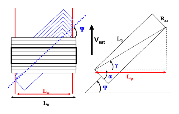
Figure 25.
Effects of the yaw angle on the interferometric swath.
Appendix 2

Appendix 2.
| B | Interferometric baseline |
| θ | View angle |
| r / R | Range |
| X | Position in the swath |
| h | Height above the tangent plane at nadir |
| α | Roll angle |
| H | Altitude of the satellite |
| Φ | Interferometric phase |
| k | Wavenumber/Boltzman constant |
| Rn/Rn | Earth radius nadir/Earth radius target |
| hreal | Height in the local frame above the ellipsoid |
| Xreal | Target position in the local frame |
| A | Ellipsoid arc between nadir and target |
| γ | Correlation between the two channels |
| N | Number of looks |
| Pt | Transmitted power |
| G | Antenna gain |
| λ | Wavelength |
| Laz | Antenna length |
| Tpulse | Chirp length |
| Bd | Chirp bandwidth |
| σ0 | Backscattering coefficient |
| L0/LΨ | Swath length |
| Raz | Azimuth resolution |
| Ψ | Yaw angle |
| β | Angle between the Sun and its projection on the orbital plane |
| ν | Angle between the projection of the Sun on the orbital plane and the satellite |
| fD | Doppler frequency |
| Vsat | Satellite velocity |
| n | Orbit pulsation |
| ρ | Atmospheric density |
| CD | Atmospheric drag coefficient |
| μ | Gravitational constant |
| a | Semi major axis |
| ΩT | Earth rotation velocity |
| XA/D | Across track coordinate in the ascending/descending local frame |
| YA/D | Along track coordinate in the ascending/descending local frame |
| Ninterferometer/nadir_altimeter/ocean/tropo_iono | Height error brought by the interferometer/nadir altimeter/ocean temporal decorrelation/tropospheric and ionospheric delays |
References
- Rodriguez, E.; Pollard, B. The measurement capabilities of wide swath ocean altimeters. HOTSWG Proceedings 2001, 190–215. [Google Scholar]
- Pollard, B.; Rodriguez, E.; Veilleux, L. The Wide Swath Ocean Altimeter: Radar Interferometry for Global Ocean Mapping with Centimetric Accuracy. AEEE Aerospace Conference Proceedings 2002, 2, 1007–1020. [Google Scholar]
- Cazenave, A.; Fu, L.-L. (Eds.) Satellite Altimetry and Earth Sciences: A Handbook of Techniques and Applications. In International Geophysics Series; 2000; Volume 69, Academic Press.
- Fu, L.-L.; Rodriguez, E. High-Resolution Measurement of Ocean Surface Topography by Radar Interferometry for Oceanographic and Geophysical Applications. International Union of Geodesy and Geophysics 2004, 19, 209–224. [Google Scholar]
- Bamler, R.; Hartl, P. Synthetic aperture radar interferometry. Inverse Problems 1998, 14, 1–54. [Google Scholar]
- Massonet, D.; Rabaute, T. Radar Interferometry: Limits and Potential. IEEE Trans. Geosci. Remote Sens. 1993, 31, 455–464. [Google Scholar]
- Gatelli, F.; Guarnieri, A.M.; Parizzi, F.; Pasquali, P.; Prati, C.; Rocca, F. The Wavenumber Shift in SAR Interferometry. IEEE Trans. Geosci. Remote Sens. 1994, 29(6), 855–865. [Google Scholar]
- Pearson, E.S.; Wishart, J. 1898-1956, Biometrica 44 (1-2); 1957; Volume 1-8, pp. 54–163. [Google Scholar]
- Bamler, R.; Just, D. Phase statistics in SAR interferograms. IGARSS 1993 Proceedings 1993, 980–984. [Google Scholar]
- Lee, J.S.; Hoppel, K.W.; Mango, S.A.; Miller, A.R. Intensity and phase statistics of multilook polarimetric and interferometric SAR imagery. IEEE Trans. Geosci. Remote Sens. 1994, 32(5), 1017–1028. [Google Scholar]
- Lee, J.S.; Miller, A.R.; Hoppel, K.W. Statistics of phase difference and product magnitude of multi-look processed Gaussian signals. Waves in Random Media 1994, 4, 307–319. [Google Scholar]
- Touzi, R.; Lopez, A. Statistics of the Stokes parameters and of the complex coherence parameters in one-look and multi-look speckle fields. IEEE Trans. Geosci. Remote Sens 1996, 34(2), 519–531. [Google Scholar]
- Touzi, R.; Lopez, A.; Bruniquel, J.; Vachon, P.W. Coherence estimation for SAR imagery. IEEE Trans. Geosci. Remote Sens. 1999, 37, 135–149. [Google Scholar]
- Abramowitz, M.; Stegun, I.A. Handbook of Mathematical Functions; New York; Dover, 1965. [Google Scholar]
- Rodriguez, E.; Martin, J.M. Theory and Design of Interferometric Synthetic Aperture Radars. IEEE Proceedings, Part F: Radar and Signal Processing 1992, 39(2), 147–159. [Google Scholar]
- Freilich, M.H.; Vanhoff, B.A. The Relationship between Winds, Surface Roughness, and Radar Backscatter at Low Incidence Angles from TRMM Precipitation Radar Measurements. Journal of Atmospheric and Oceanic Technology 2003, 20(4), 549–562. [Google Scholar]
- Freilich, M.H.; Challenor, P.G. A new approach for determining fully empirical altimeter wind speed model functions. J. Geoph. Res. 1994, 99, 25051–25062. [Google Scholar]
- Wentz, F.J.; Peteherych, S.; Thomas, L.A. A model function for ocean radar cross-sections at 14.6 GHz. J. Geophys. Res. 1984, 89, 3689–3704. [Google Scholar]
- Jackson, F.C.; Walton, W.T.; Hines, D.E. Sea Surface mean square slope from Ku-band backscatter data. J. Geophys. Res. 1992, 97, 11411–11427. [Google Scholar]
- Zarrouati, O. Trajectoires spatiales, Centre National d'Etudes Spatiales, Cepadues Editions ed; 1987. [Google Scholar]
- Sardon, E.; Rius, A.; Zarraoa, N. Estimation of the Transmitter and Receiver Differential Biases on the Ionospheric Total Electron Content from Global Positioning System Observations. Radio Science 1994, 29, 577–586. [Google Scholar]
- Ruffini, G.; Cardellach, E.; Flores, A.; Cucurull, L.; Rius, A. Ionospheric Calibration of Radar Altimeters Using GPS Tomography. Geophys. Res. Lett. 1998, 25(20), 3771–3774. [Google Scholar]
- Wentz, F.J. A well-calibrated ocean algorithm for SSM/I. J. Geophys. Res. 1997, 102(C4), 8703–8718. [Google Scholar]
- Zanife, O.Z.; Dumont, J.P.; Thibaut, P.; Vincent, P.; Carayon, G.; Steunou, N. 2002: Preliminary comparison of the Topex and Poséidon-2 Radar Altimeters. Jason-1/Topex/Poséidon Scientific Working Team Meeting, New-Orleans, Louisiana USA, 21-23 October 2002.
- Ducet, N.; Le Traon, P.Y.; Reverdin, G. Global High Resolution Mapping of Ocean Circulation from Topex/Poseidon and ERS1/EES2. J. Geophys. Res. 2000, 105(C8), 19477–19498. [Google Scholar]
- Imel, D.A. Evaluation of the Topex/Poseidon dual-frequency ionosphere correction. J. Geophys. Res. 1994, 99(12), 24895–24906. [Google Scholar]
- Chelton, D.B.; deSzoecke, R.A.; Schlax, M.G.; Naggar, E.; Siwertz, N. Geographical variability of the first baroclinic Rossby radius of deformation. J. Phys. Oceanograph. 1998, 28, 433–460. [Google Scholar]
- Mourre, B.; De Mey, P.; Lyard, F.; Le Provost, C. Assimilation of sea level data over continental shelves: an ensemble method for the exploration of model errors due to uncertainties in bathymetry. Dynamics of Atmospheres and Oceans 2004, 38, 93–121. [Google Scholar]
- Parke, M.E.; Stewart, R.L.; Farless, D.L.; Cartwright, D.E. On the choice of orbits for an altimetric satellite to study ocean circulation and tides. J. Geophys. Res. 1987, 92(11), 693–11707. [Google Scholar]
- Le Provost, C. Tides over ridges, shelves, and near the coasts, in Report of the High-Resolution Ocean Topography Science Working Group Meeting; Red. 2001-4; Chelton, D.B., Ed.; Oregon State University: Corvallis, OR; p. 224 pp.
- Le Provost, C. Generation of overtides and compound tides (review). In Tidal Hydrodynamics; Parker, B., Ed.; John Wiley and Sons: New-York, 1991; pp. 269–296. [Google Scholar]
- Centre National d'Etudes Spatiales, Spacecraft Techniques and Technology2005; Volume 2, Cepadues Editions ed.
- Phalippou, L.; Guijarro, J. End to end Performances of a Short Baseline Interferometric Radar Altimeter for Ocean Mesoscale Topography. IGARSS 2004 Proceedings 2004. [Google Scholar]
- Phalippou, L.; Cotton, D.; Guijarro, J.; Menard, Y.; Vincent, P. Future radar altimeter concepts for ocean applications. IGARSS 2003 Proceedings 2003. [Google Scholar]
© 2006 by MDPI ( http://www.mdpi.org). Reproduction is permitted for noncommercial purposes.