Determination of the Temperature Change by Means of an Outcoming Signal of Electric Resistance in an Isoperibolic Calorimetric Cell. Obtainment of Heat Solution

Abstract

An isoperibolic calorimetric cell is built with glass surrounded by plastic insulation. The cell has a lid on which a thermistor thermometer, an electric resistance to provide the cell with definite quantities of electric work and a container for a glass ampoule, are placed. For measuring the thermal changes, an NTC thermistor, which provides an electric resistance signal that varies with temperature, is used. Calibration curves of the thermistor and of the stabilization of the system signal in thermal equilibrium are shown, which enable the observation of a good insulation. The calorific capacity of the system with water, with a value of 206.7 ±0.7 J °C^-1 is determined; the solution enthalpy for propanol-water and KCl-water systems is obtained, which shows the behavior of the cell before exothermic and endothermic effects, respectively.

1. Introduction

The calorimetry of solution can involve, totally or partially, processes of solution, mixture and dilution, which generate an amount of heat in the liquid solution at a definite temperature [1]. The solution enthalpy is generally measured in calorimeters with heat shield, in which the temperature of the calorimetric cell changes with the development of the process, while the temperature of the surroundings is kept constant by means of a thermostat [2]. Since the operating conditions are not strictly adiabatic, these equipments were called isoperibolic calorimeters by Kubaschewski and Hultgren [3], and, since then, they are distinguished from isothermal and adiabatic calorimeters.

In isoperibolic calorimeters, it is intended to reduce the heat exchange between the cell, where the process takes place, and the surroundings. This is achieved by minimizing the difference in temperature between them, thus diminishing the thermal transference coefficient and reducing the time for the heat exchange.

When the thermal transference between the surroundings and the cell is limited, so that the heat exchange depends on the temperature difference between them, T_A corresponds to the temperature of the surroundings and T_C to the temperature of the cell and measurement system. Since T_A is constant, then the heat flow is a function of T_C. If the heat generation inside the cell ends, the temperature T_C gets close to the temperature of the surroundings T_A [4].

At the beginning of the experience, the temperature is kept very close to the temperature of the surroundings T_A. When a certain amount of heat is produced in the cell, the temperature raises first, then reaches a top value, to finally start to descend because T_C is larger than T_A, and the magnitude of descent depends on the insulation of the cell. In macro isoperibolic calorimeters, it is intended to keep the thermal transference as low as possible, so that the heat measurement in such devices is very similar to the one made in an adiabatic system. The heat amount for the process examined is equal to:

$$\text{Q}=\text{Cp}\mathrm{\Delta }{\text{T}}_{\text{corrected}}$$

(1)

Where Cp is the calorific capacity of the system studied plus the calorific capacity of the cell, ΔT_corrected is the temperature difference for which a graphic correction is made because of the small but existing heat leak [5,6]. For exact measurements, it is not completely necessary to maintain the heat leak as low as possible, it is enough that they can be reproduced according to the temperature difference between the cell and the surroundings [7] and that they can be determined by electric calibrations.

Given the fact that, during the calorimetric experience it is necessary to follow, with the best possible sensitivity, the temperature variation of cell T_C, on which the evaluation of the heat generated by the studied process depends, easy to handle electronic thermometers are used, with a previous calibration according to the temperature. The thermistors are frequently used in calorimetry, and are made with semiconductor ceramic materials and with mixtures of powders of metallic oxides treated at high pressures and temperatures [8].

In thermistors, an electric resistance signal that does not depend lineally on the temperature and that in many cases has an inverse relation is measured. Thus, they are referred to as thermistors with negative temperature coefficient, NTC. A relation that is established between the resistance of the thermistor and the temperature is:

$$R_T=R_{\infty }{e}^{(B/T)}$$

(2)

where T is the system temperature in °C; R_T is the resistance of the thermistor at temperature T; R_∞ and B are constants which depend on the characteristics of the thermistor [9].

In this work, an isoperibolic calorimetric cell is connected to an NTC thermistor for measuring the heats of solution of liquids and solids, in which small temperature's magnitudes are determined.

2. Experimental Section

2.1. Isoperibolic calorimetric cell

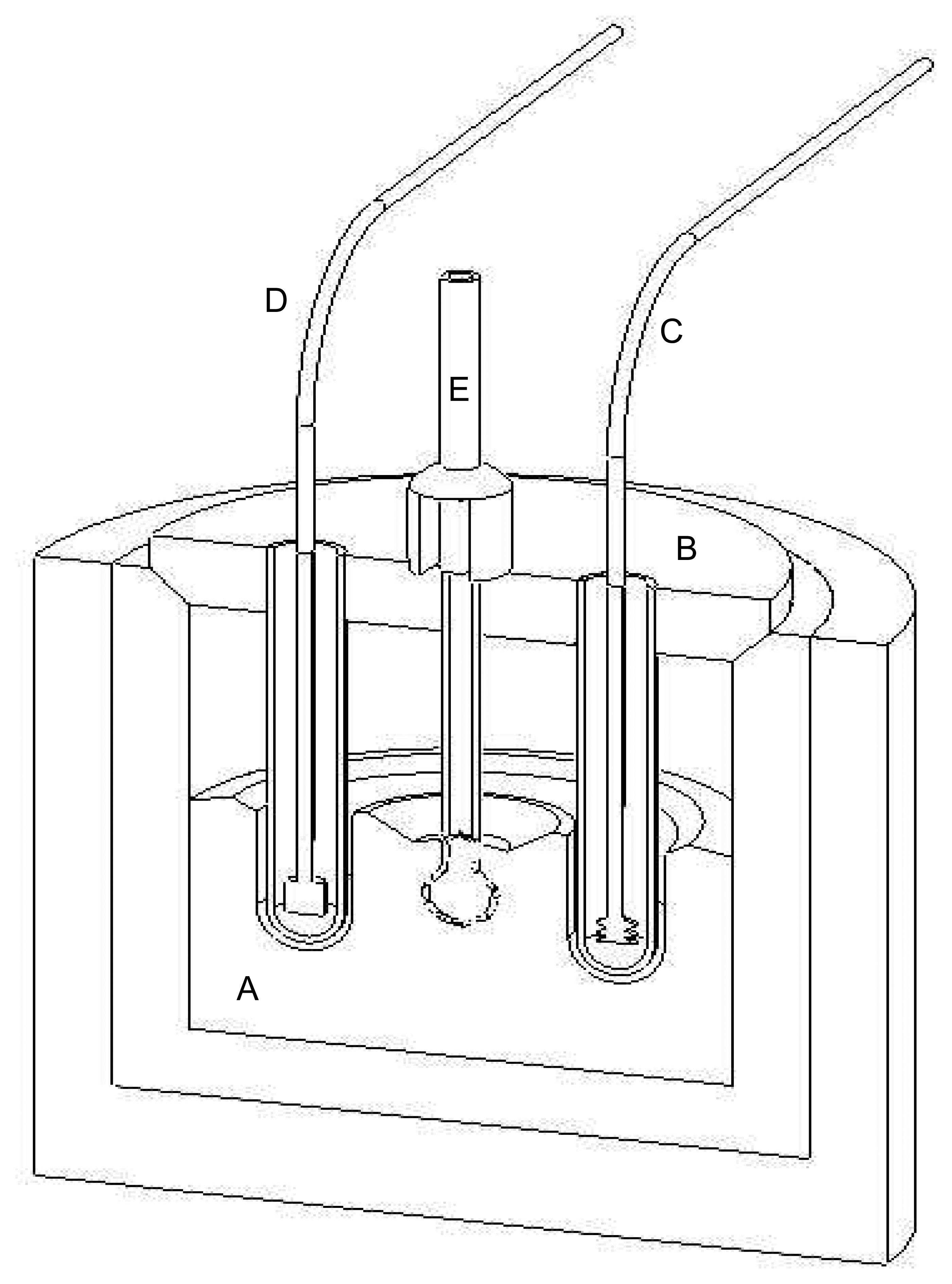
The calorimetric cell is composed of a cylindrical Pyrex glass container 45 mm. in diameter and 45 mm in height, with a capacity of approximately 60 mL (A); in the internal upper part, a 6 mm section is ground to adjust a lid, also made of glass (B), with holes which allow for the placement of two glass tubes which contain, one which electric resistance is of 150 ohms and 5 watts for heating the inside of the cell (C), and the other which the NTC thermistor thermometer is of 1.00 KΩ at 25 °C (D). A third hole in the lid permits the placement of a glass ampoule where the solute is placed to obtain the solution (E). The above mentioned cell is placed, with a good thermal contact, inside a plastic block of 125 mm. in diameter and 85 mm in height. A hole is made in the center of the block with the dimensions of the cell. Figure 1 shows a diagram of the cell used.

The above set is placed inside an air thermostat that maintains constant the temperature of ± 0.1 °C, to make the calorimetric determinations.

2.2. Calibration of the thermistor

Approximately 100 mL of water, at a temperature between 0 y 50 °C, is placed inside a Dewar cell. A plastic lid is adjusted to the glass Dewar vessel where, inside a glass Pyrex tube of 7 mm in diameter and 20 cm in length, the thermistor thermometer is placed connected to copper connectors for the reading of the outgoing electric resistance and a mercury thermometer with 0.01°C accuracy, calibrated and with register NIST (National Institute of Standards and Technology), and the cell is closed. Readings of the outgoing electric resistance, in KΩ, are made for the thermistor with a precision multimeter Hewlett-Packard 34401A with a sensitivity of 0.01 ohm and, simultaneously, the temperature readings are made with the mercury thermometer.

2.3. Determination of Stability in the Electric Resistance Reading

Distilled water (40 mL) is placed inside the cell, at a temperature close but above 25 °C, to establish the change that is produced in the system temperature at a specific time. Readings of outgoing electric resistance of the thermistor in function to time are made for 60 minutes periods, with recordings of resistance readings every 20 minutes, in order to observe the continuous change in the electric resistance of the thermistor and the insulation of the cell-water system. Resistance curves in function to time are determined, with the calorimetric set kept at room temperature and with temperature control inside the thermostat.

2.4. Determination of the Heat Capacity of the Cell-Water System

Determination of the heat capacity is carried out by placing 40mL of distilled water at approximately 25 °C inside the glass cell. The cell is placed inside the insulator and the entirety is taken to the air thermostat which keeps the temperature at 25 ± 0.1 °C. When the system reaches thermal equilibrium, readings of electric resistance are taken in function to time, every 30 seconds for a period of around 10 minutes, during which the outgoing resistance of the thermistor remains constant. After this time, electric work is provided to the cell through the heating resistance, and the resistance readings continue until they are constant again.

2.5. Determination of the heat solution

Once the characteristics of the calorimetric cell are known, the determinations of the heat solution are made for a system in liquid phase, propanol-water and for a solid liquid KCl-water system. Water (40 mL) is placed in the cell and in the glass ampoule an amount of the solute is weighed with a precision of 0.001 g; the cell is assembled and is thermally equilibrated in a thermostat at 25 ± 0.1 °C, for approximately one hour. When the variation in the outgoing electric resistance of the thermistor is constant, its readings are started for a pre-period between 10 and 15 minutes, with resistance readings every 20 seconds; then the mixture of the solvent, water, and the solute is made, the resistance readings are continued until they become constant and finally it is calibrated electrically.

3. Results and Discussion

The determination of the change of temperature that occurs inside the cell, in isoperibolic calorimetry, is an important factor as well as its insulation, so that the largest amount of heat developed inside can be detected by the system adapted for the measuring. Isoperibolic calorimeters have the advantage of a rather simple building and operation, and the results obtained are due to the combination of an adequately insulated cell and a sensitive thermometer easy and rapid to read [10].

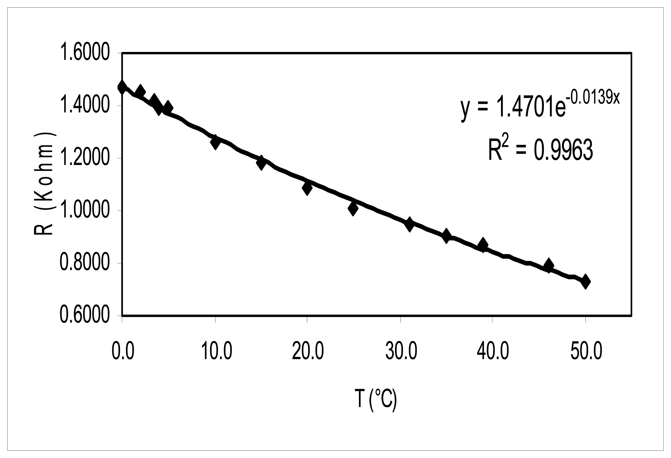
Figure 2 corresponds to the relation between the outgoing electrical resistance of the thermistor and the temperature obtained in a mercury thermometer of 0.01 °C. It can be observed that there is an exponential correlation between the temperature in °C and the electric resistance recorded in the multimeter with an accuracy of 0.01Ω, in the calibration range observed of 0 to 50 °C and that permits the observation of temperature variations of 0.001 °C.

The equation that describes the experimental points is R = 1.4701e^−0.0139Twith a correlation coefficient r², of 0.9963, which reflects the behavior of the NTC thermosensor, where, when the temperature increases, the electric resistance diminishes. The points show low dispersion and a continuous diminishing of the resistance with temperature that makes the thermistor an element with an adequate thermometric property that responds noticeably to temperature [11]. And, since in isoperibolic calorimetry temperature differences are evaluated, the use of the thermistor thermometer facilitates the study of systems where temperature changes are observed in ranges near room temperature, as in the case of the calibration made.

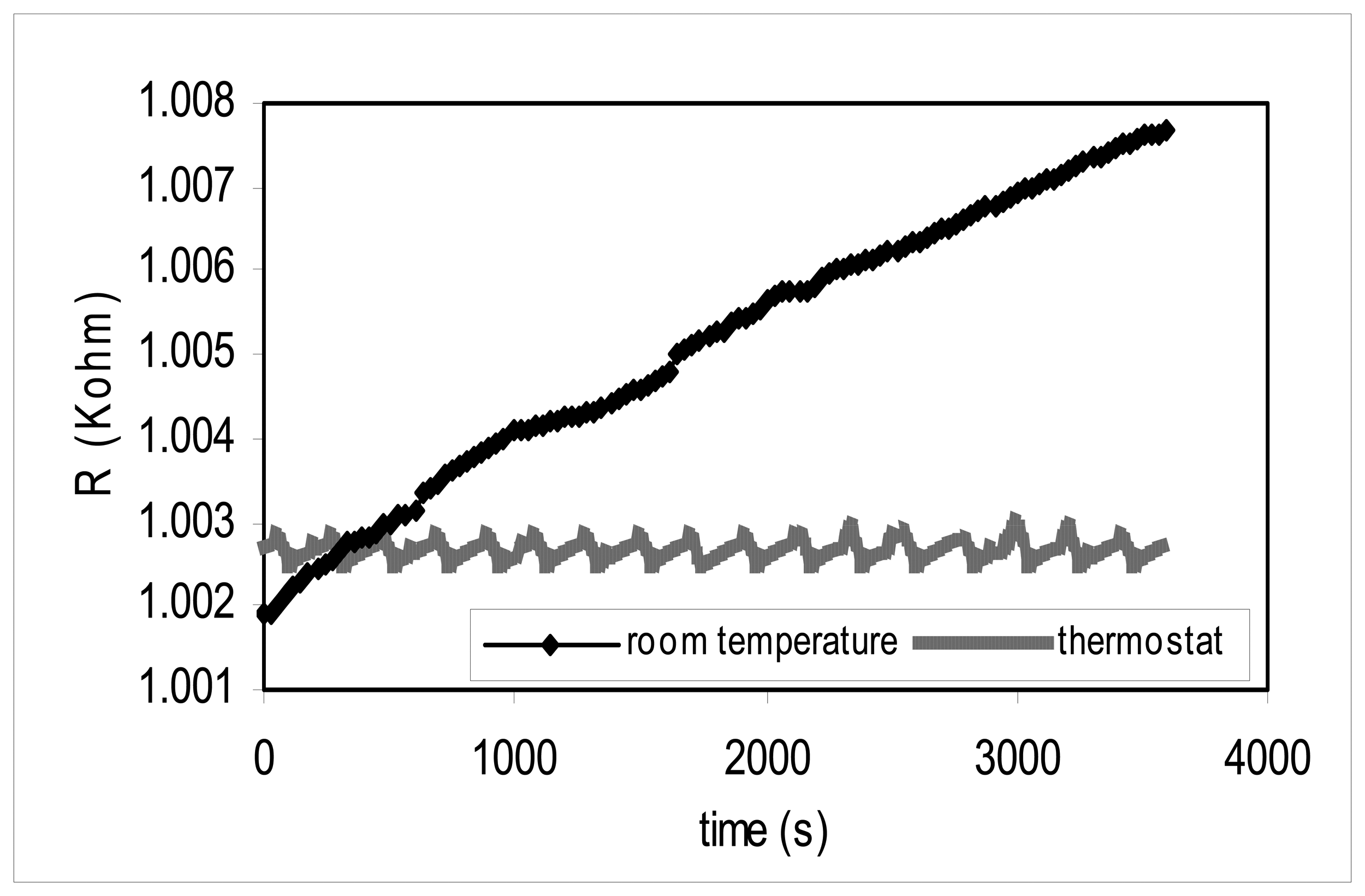
Figure 3 shows two curves of outgoing electric resistance of the thermistor in function to the time. The black line corresponds to the register of the heat losses when the calorimetric unit, with water inside the cell, is at room temperature with a value of approximately 20 °C. The 40 mL of water placed in the cell should have a higher temperature, of approximately 27.5 °C, so that a thermal transference favored by the temperature gradient may occur. The register shows a variation in the outgoing electric resistance of the thermistor, from 1.00191 to 1.00765 KΩ, which indicates the cooling of the system and produces a temperature variation of 0.414 °C in one hour. This shows the good insulation of the cell.

The register in grey in Figure 3 is produced when the calorimetric unit is placed in a thermostat with a temperature adjusted at 26 °C, that is with a difference of around 2 °C with respect to the conditions of the cell; small variations occur with resistance values between limits during the hour of observation and the largest change observed is of 5 Ω. The result indicates that it is advisable to make the calorimetric determinations by controlling the temperature of the surroundings and confirms the adequate insulation of the cell to operate under isoperibolic conditions.

The parameter that needs to be known is the cell constant that, in this case, corresponds to its heat capacity [10]. For this purpose, an amount of electric work is dissipated in the cell and the change in temperature is evaluated.

Table 1. Determination of the Heat Capacity of the Cell-Water System at 25.0 °C.

Vc (Volt)	Welec (J)	ΔT (°C)	Cp (J °C-1)
10.2	97.92	0.483	207.2
10.0	102.0	0.495	206.1
12.1	153.1	0.738	207.5
12.2	146.4	0.712	205.6
15.2	200.6	0.968	207.2
15.3	201.9	0.978	206.4
18.0	248.4	1.199	207.2
18.2	251.2	1.215	206.7
20.1	301.5	1.455	207.2
19.9	298.5	1.452	205.6

shows the results obtained for the heat capacity of the system with water, when it dissipates in the calorimetric cell, thus increasing amounts of electric work. The table shows the heating potential provided to the heating resistance, Vc in volt; the electric work dissipated, Welec in J, the temperature difference generated, ΔT in °C and the heat capacity of the cell-water system, Cp in J°C^-1.

The results show that considerable temperature differences can be determined, from approximately 0.480 °C, that take place in the cell because of the energetic change. The values obtained for the heat capacity of the system are reproducible at different levels of dissipated electric work, which indicates that the cell is appropriate for the determination of enthalpic changes between 100 to 300 J. When making the statistical treatment of the values of Cp of the system, an average value of 206.7 J °C^-1 is obtained, with a standard deviation of ± 0.7 J °C^-1. Knowing the water content, a value of 39.3 J °C^-1 is found for the calorimetric cell.

Figure 4 shows a curve of outgoing electric resistance of the thermistor in function to the time, when an electric work of around 150 J is dissipated in the cell. This graph represents a typical thermogram produced by an exothermic effect; in this case the reduction in the electric resistance is caused by the characteristics of the thermistor. Its resistance variation is inversely proportional to the temperature. Likewise, a constant resistance in the initial and final periods is observed, as expected for an isoperibolic cell [4, 6, 12].

The heat solution is determined for propanol-water and KCl-water systems with the calorimetric cell built. These systems are used as reference since the enthalpy values of the solution can be compared with the literature [10, 13, 14].

Table 2. Determination of the Enthalpy of Solution of Propanol in Water at 25 °C.

Molality (mol kg-1)	ΔT (°C)	Q (J)	ΔHsln (kJ mol-1)
0.099	0.203	-41.96	-10.40
0.198	0.416	-86.16	-10.81
0.294	0.639	-132.5	-11.09
0.391	0.873	-181.0	-11.37

shows the results obtained in the determination of the heat solution for different amounts of propanol in 40 mL of water at 25.0 °C. It shows the molality of the solution, m in mol kg^-1; the difference in temperature generated, ΔT in °C; the heat generated in the solution, Q in J and the change in the enthalpy of solution, ΔH_sln in kJ mol^-1.

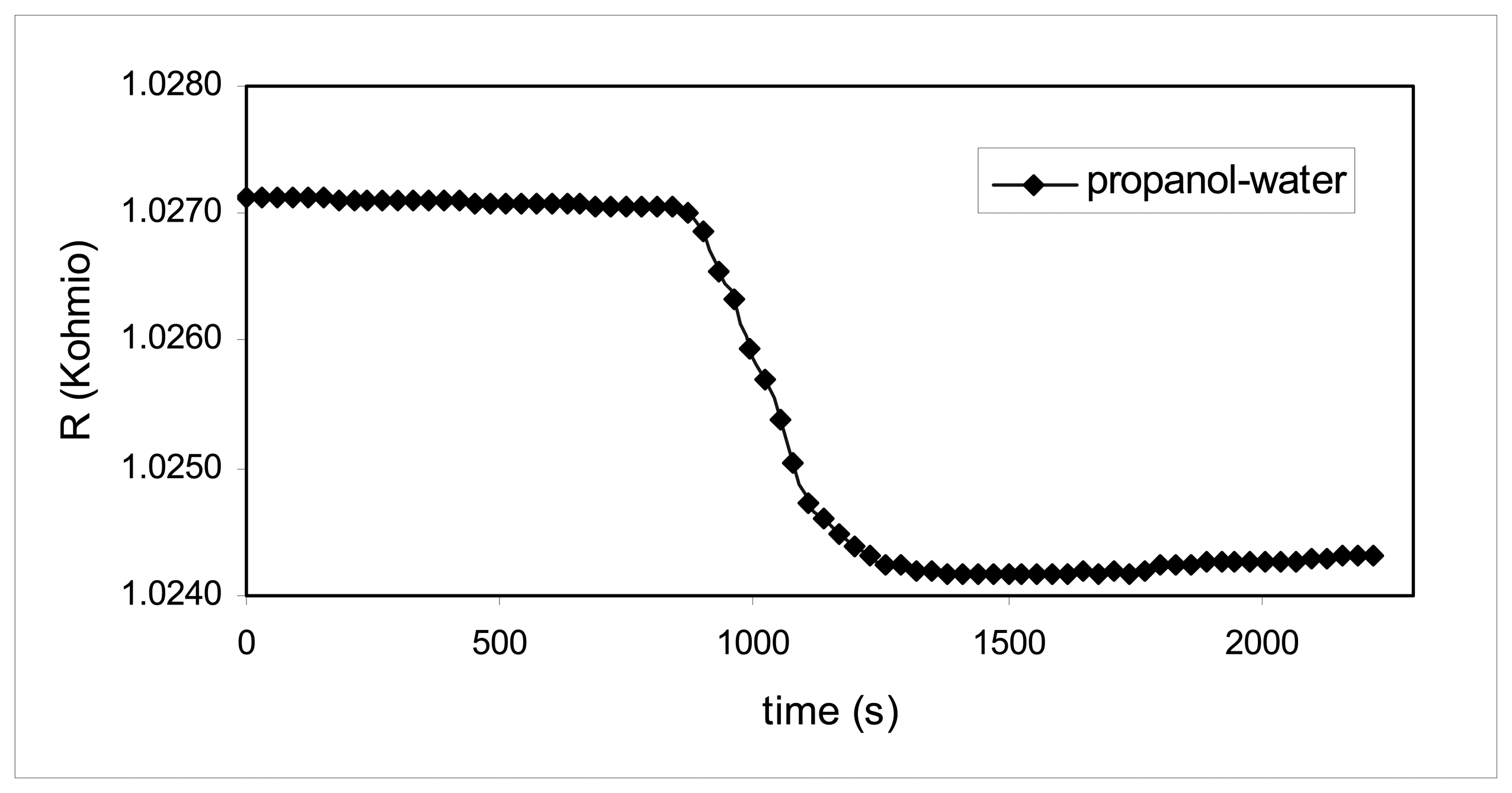
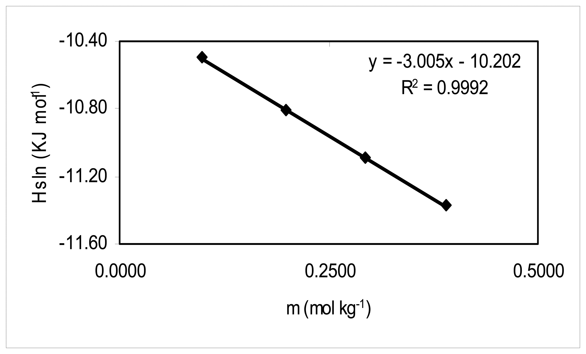
The results show interesting aspects, the first corresponding to the determination of ΔT which is achieved with the thermistor for small temperature changes. And, as can be observed in Figure 5, the thermogram obtained for the solution with the lowest concentration, said change can be easily evaluated. The other aspect, related to the one above, is that relatively small heat solution, around 40 J, can be determined. Finally the variation of the enthalpy of solution ΔH_sln, with the concentration of the solution that indicates its dependence on the quantity of alcohol, is observed. Thus, in order to compare, the enthalpy of solution at infinite dilution ΔH^∞_sln, is calculated, which is obtained as the limit when the quantity of propanol tends to zero in a ΔH_sln graph, in function to the molal concentration of the solution, as shown in Figure 6. The experimental points show a lineal relation, with an equation ΔH_sln = -3.005m – 10.202 and a correlation coefficient, r², of 0.9992. We have then an enthalpy of solution at infinite dilution for propanol in water of –10.202 kJ mol^-1, which is in agreement with literature [13].

Table 3. Determination of the Enthalpy of Solution for KCl in Water at 25 °C.

Molarity (mol kg1)	ΔT (°C)	Q (J)	ΔHsln (kJ mol-1)
0.071	0.244	50.34	17.55
0.069	0.238	49.05	17.54
0.071	0.242	49.93	17.55
0.070	0.240	49.48	17.55
0.070	0.203	49.41	17.55
0.070	0.240	49.50	17.55

shows the results for the determination of the enthalpy of solution of the system KCl-water, with the same variables and units presented in Table 2.

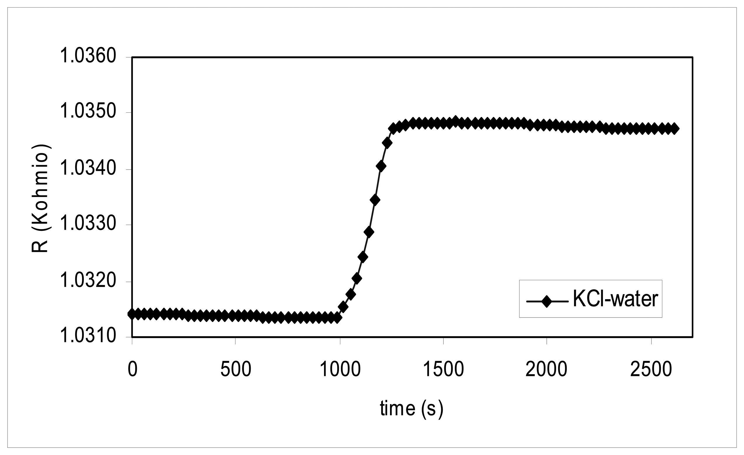
The determination of the enthalpy of solution of KCl in water is made for the same amount of salt, around 0.210 g, in order to observe the reproducibility obtained in the determinations when small heat absorptions are produced, like when the process is endothermic. Figure 7 presents the thermograph obtained, where a convenient evaluation of temperature change can be made. The statistical processing of the data results in an average value of 17.551kJ mol^-1 with a standard deviation of 1.51×10^-3kJ mol^-1. Again, the value obtained for the enthalpy of solution of KCl is in agreement with literature [14].

4. Conclusions

A calorimetric cell is built with glass inside plastic insulation, with a capacity of approximately 60mL, which operates in isoperibolic conditions. The calorific capacity of the cell has a value of 39.3 J °C^-1.

An NTC thermistor thermometer is connected and the changes of electric resistance generated are read with a precision multimeter. Small changes of temperature are determined and a rapid response of the thermometer to these changes occurs.

The calorific capacity of the system with water at 25.0 °C is determined, with a result of 206.7 ± 0.7 J °C^-1.

The enthalpy of solution for the systems propanol-water and KCl-water is determined. In the former case, a value of –10.202 kJ mol^-1 is obtained for the enthalpy of solution at infinite dilution, and for the salt, a value of 17.551± 1.51×10^-3 kJ mol^-1.