
ECG Sensor Design Assessment with Variational Autoencoder-Based Digital Watermarking


Abstract
1. Introduction
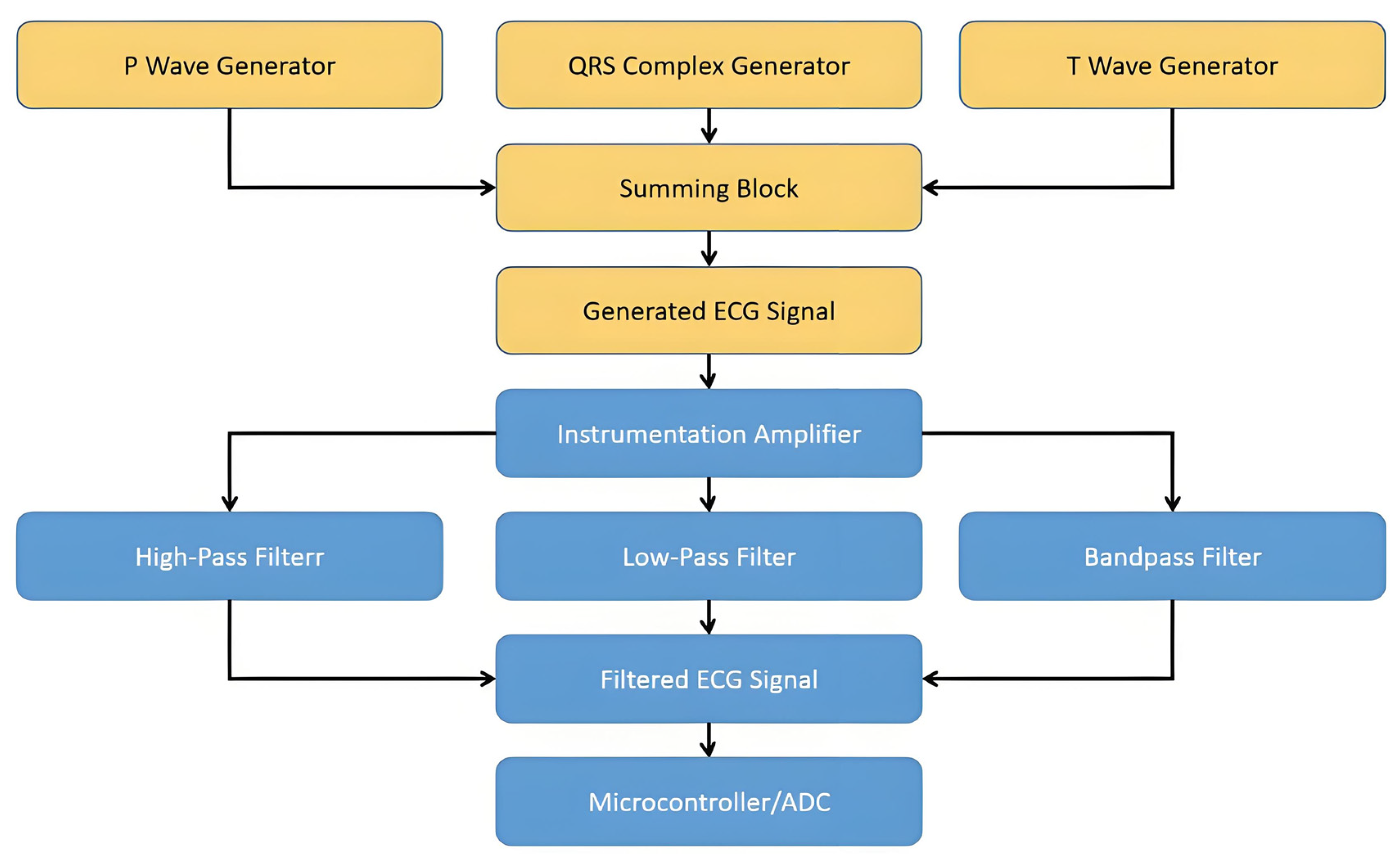
- High-Pass Filter: a cutoff frequency of 1.0 Hz
- Low-Pass Filter: a cutoff frequency of 10.0 Hz
- Band-Pass Filter: a low cutoff frequency of 5.0 Hz and a high cutoff frequency of 20.0 Hz
2. Variational Autoencoders (VAEs)
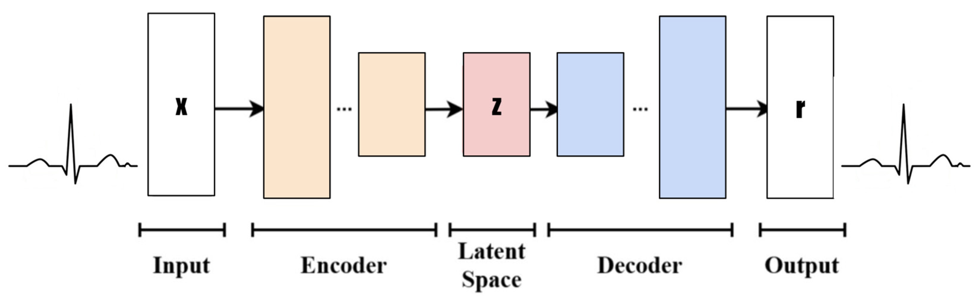
- Input: Design a rectangle or ellipse with “Input” inside. The data type is the time-series ECG signal (x) and the dimension (1, 100).
- Encoder: Use multiple rectangles or trapezoid stacks to represent the encoder layer. Each rectangle can be simply marked with “Enc Layer” or a specific layer name (such as the convolution layer, pooling layer, etc.), and arrows indicate the data flow direction.
- Latent Space: This is represented by a circle or oval, with “Latent Space” marked inside. You can add some small dots or cloud patterns to symbolize potential representation.
- Decoder: This is similar to the encoder design but in the opposite direction, and it means decoding data from the latent space back to the original or target domain.
- Output: The type of output data (reconstructed x) and dimension (1, 100) are labeled “Output”.
2.1. VAE Mathematical Description
2.2. Variational Reasoning
2.3. Autoencoder
2.4. Loss Function
- Reconstruction Error: This measures the difference between the reconstructed and the original . Commonly used metrics for this purpose are the Mean Squared Error (MSE) or Binary Cross-Entropy (BCE), depending on the nature of the data being reconstructed.
- KL Divergence: This measures the difference between the approximate posterior distribution and the prior distribution . KL Divergence, also known as Kullback–Leibler Divergence, is a measure of how one probability distribution diverges from another. In the context of VAEs, minimizing this divergence encourages the approximate posterior to resemble the prior distribution, typically a simple distribution like a multivariate Gaussian, facilitating the generation of new samples.
3. Methodology
3.1. Data Preparation and Preprocessing
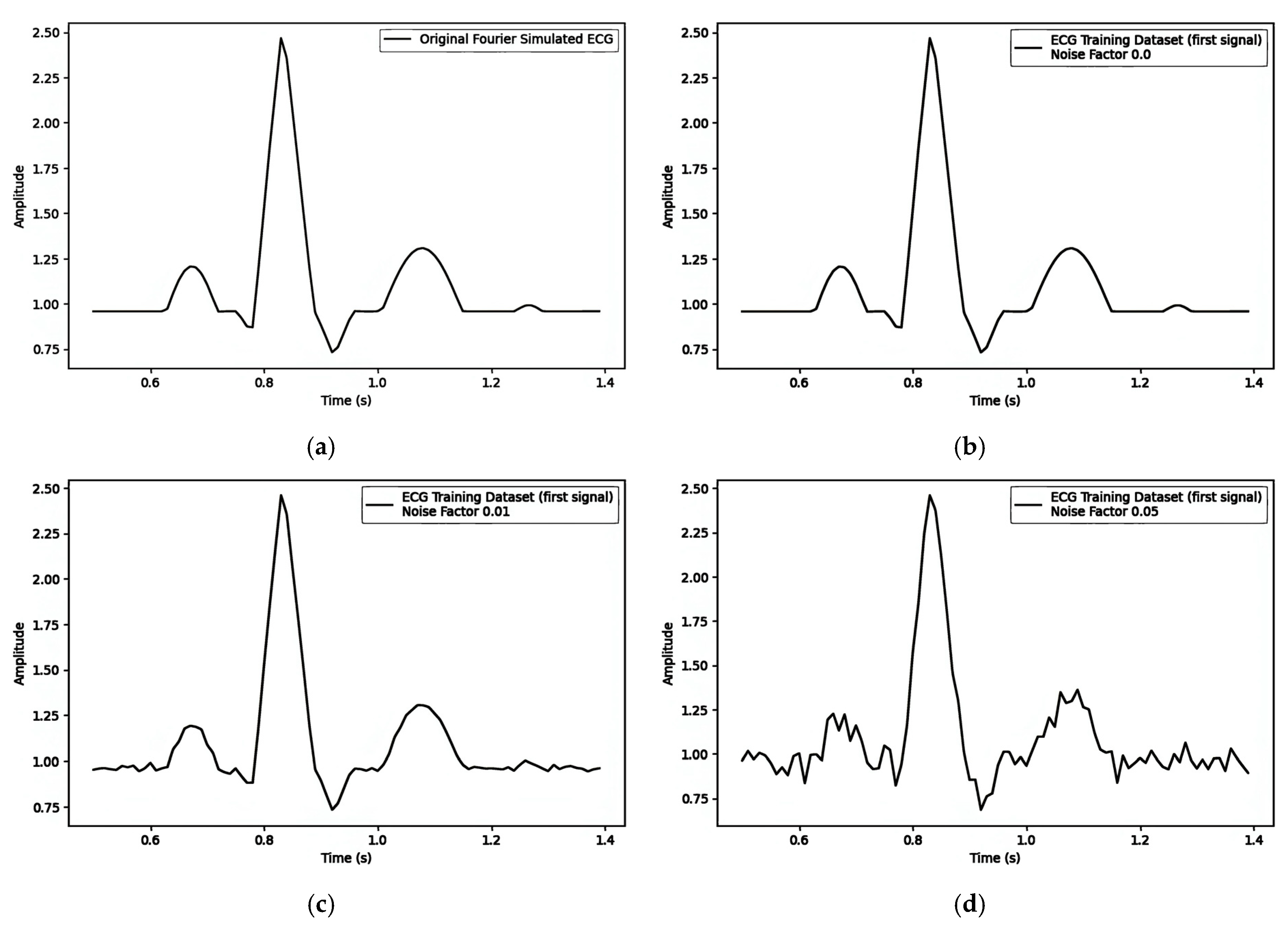
Fourier-Simulated ECG
- P Wave: The P wave represents atrial depolarization, with the electrical signal preceding atrial muscle contraction. It typically lies above the isoelectric line, and its morphology and amplitude can provide insights into atrial size and conduction abnormalities.
- PR Interval: The PR interval measures the time from the onset of the P wave to the start of the QRS complex, reflecting the duration of electrical signal conduction from the atria to the ventricles. During the PR interval, the ECG typically displays the isoelectric line, indicating that ventricular depolarization has not yet begun.
- QRS Complex: The QRS complex represents ventricular depolarization, which is the most prominent and substantial part of the ECG. It consists of three waves (Q, R, and S), though not every QRS complex fully exhibits all three. The isoelectric line preceding the QRS complex signifies the absence of ventricular depolarization, while the subsequent isoelectric line may indicate the completion or imminent onset of ventricular repolarization.
- ST Segment: The ST segment connects the end of the QRS complex to the beginning of the T wave, reflecting the early phase of rapid ventricular repolarization. In normal conditions, the ST segment should be level with or slightly below the isoelectric line without significant deviation. Changes in the ST segment (e.g., elevation or depression) are crucial indicators of myocardial ischemia or infarction.
- T Wave: The T wave represents the slow repolarization of the ventricles and the electrical signal as ventricular muscle cells gradually return to their resting potential after contraction. The direction and amplitude of the T wave can be influenced by various factors, including myocardial metabolic status, medication effects, and electrolyte balance.
- QT Interval: The QT interval measures the time from the onset of the QRS complex to the end of the T wave, encompassing the total duration of ventricular depolarization and complete repolarization. The prolongation or shortening of the QT interval may be associated with arrhythmia, electrolyte disturbances, or medication effects.
- U Wave: Following the T wave, with an interval of 0.02 to 0.04 s, the U wave is wide, low, and typically has an amplitude below 0.05 millivolts and a duration of approximately 0.20 s.
3.2. Watermarking Modes in VAEs
3.2.1. Pre-Reconstruction: Embedding into the Mean ()
- Embedding Process
- (a)
- Encoding: Pass the ECG segment through the encoder to obtain and .
- (b)
- Watermark Integration: Concatenate or add a scaled watermark to the mean where is the embedding strength.
- (c)
- Reparameterization: Sample the latent variable using and :
- (d)
- Decoding: Pass to the decoder to generate the watermarked ECG signal .
- Extraction Process
- (a)
- Decoding: When verifying, encode the suspected watermarked ECG again to obtain .
- (b)
- Watermark Retrieval: Compute the difference between the original (if known or stored) and : This reverses the embedding operation and recovers the watermark.
- Notes and Trade-offs
- (a)
- Advantages: Advantages include strong invisibility and minimal additional computation.
- (b)
- Disadvantages: Disadvantages include the fact that it requires knowledge of the original mean for exact extraction; a large could degrade reconstruction quality.
3.2.2. Pre-Reconstruction: Embedding Through the Latent Variable ()
- Embedding Process
- (a)
- Encoding: Obtain and from the encoder.
- (b)
- Reparameterization: Sample the initial latent variable .
- (c)
- Watermark Integration: Add a scaled watermark to :
- (d)
- Decoding: Pass to the decoder to generate the watermarked ECG signal .
- Extraction Process
- (a)
- Re-encode: Encode the watermarked ECG to obtain .
- (b)
- Retrieval: Subtract the original from (if is available) or compare it with known references:
- Notes and Trade-offs
- (a)
- Advantages: Advantages include the fact that it preserves without modification, potentially simplifying certain aspects of the retrieval.
- (b)
- Disadvantages: Disadvantages include that the process must handle storing or recomputing the original ; increasing may introduce more distortion.
3.2.3. Post-Reconstruction: Frequency-Domain Watermarking
- Embedding Process
- (a)
- VAE Reconstruction: Generate the reconstructed ECG from a latent vector.
- (b)
- Fourier Transform: Convert to the frequency domain (e.g., via Fast Fourier Transform, FFT).
- (c)
- Watermark Insertion: Modify selected frequency coefficients based on the watermark bits. For instance,
- ▪
- If watermark bit = 1, increase the magnitude by .
- ▪
- If watermark bit = 0, decrease the magnitude by .
- (d)
- Inverse Transform: Apply the inverse FFT to obtain a watermarked ECG signal in the time domain.
- Extraction Process
- (a)
- Fourier Transform of Watermarked ECG: Convert the watermarked signal back to the frequency domain.
- (b)
- Compare Coefficients: Check how each targeted coefficient changes relative to a reference (either an original or a threshold-based approach).
- (c)
- Reconstruct Watermark Bits: If a coefficient is higher than expected, interpret that as bit 1; otherwise, interpret it as bit 0.
- Notes and Trade-offs
- (a)
- Advantages: Advantages include the fact that there is generally minimal impact on time-domain clinical features if embedding is performed carefully; there is robust to minor time-domain noise.
- (b)
- Disadvantages: Disadvantages include more computational steps (FFT and IFFT); detection requires frequency-domain analysis and may be vulnerable to frequency-specific attacks (e.g., notch filtering).
4. Experimental Results and Discussions
4.1. Simulated Dataset
4.2. Model Evaluation Metrics
Mean Squared Error (MSE)
- is the actual value of the original signal at the th observation.
- is the predicted or generated value of the signal at the th observation.
- is the total number of observations.
4.3. Implementation of Variational Autoencoder (VAE) Architecture
4.4. Experimental Setup and Parameter
- Hardware and Software
- ○
- Implement the VAE and watermarking algorithms in Python 3.12, leveraging deep learning frameworks (e.g., PyTorch 1.8, TensorFlow 2.5).
- ○
- Use GPU acceleration for efficient model training (e.g., NVIDIA RTX GPUs).
- Hyperparameters for VAE Training
- ○
- Batch Size: Batch size is typically 16–64, depending on GPU memory.
- ○
- Learning Rate: The learning rate is often between 1 × 10⁻⁴ and 1 × 10⁻³.
- ○
- Number of Epochs: the number of epochs is 100–300, monitored by early stopping criteria.
- ○
- Latent Dimension: This is selected based on signal complexity; common ranges are 8–64.
- Watermark Parameters
- ○
- Watermark Length: This must fit the latent representation size (for pre-reconstruction) or the number of frequency coefficients (for post-reconstruction).
- ○
- Embedding Strength (α): This is critical for controlling the balance between watermark visibility and robustness. Typical test values are {0.1, 0.5, 0.9}.
- ○
- Watermark Data: These could be binary patterns, textual identifiers, or random noise vectors.
- Evaluation Metrics
- ○
- Signal Fidelity:
- ▪
- The MSE between original and reconstructed signals.
- ▪
- PSNR or SSIM (optional) are used to evaluate signal quality more comprehensively.
- ○
- Watermark Detection:
- ▪
- The accuracy/success rate of extracting the correct watermark bits is considered.
- ▪
- Threshold-based or correlation-based detection strategies are used if the watermark is noise-like.
- ○
- Robustness Tests: Noise is applied.
- Attack Scenarios
- ○
- Introduce signal manipulations (e.g., Gaussian noise and low-pass filtering) to test whether the watermark can still be detected under realistic conditions.
4.5. Watermarking Experiment Results and Discussions
- Embedding the watermark in the mean () results in α having an influence of less than on the MSE.
- Embedding the watermark through the latent variable () results in α having an influence of less than on the MSE.
- Embedding the watermark through the frequency domain results in α having an influence of less than on the MSE.
4.5.1. Embedding the Watermark in the Mean (μ)
4.5.2. Embedding the Watermark Through the Latent Variable ()
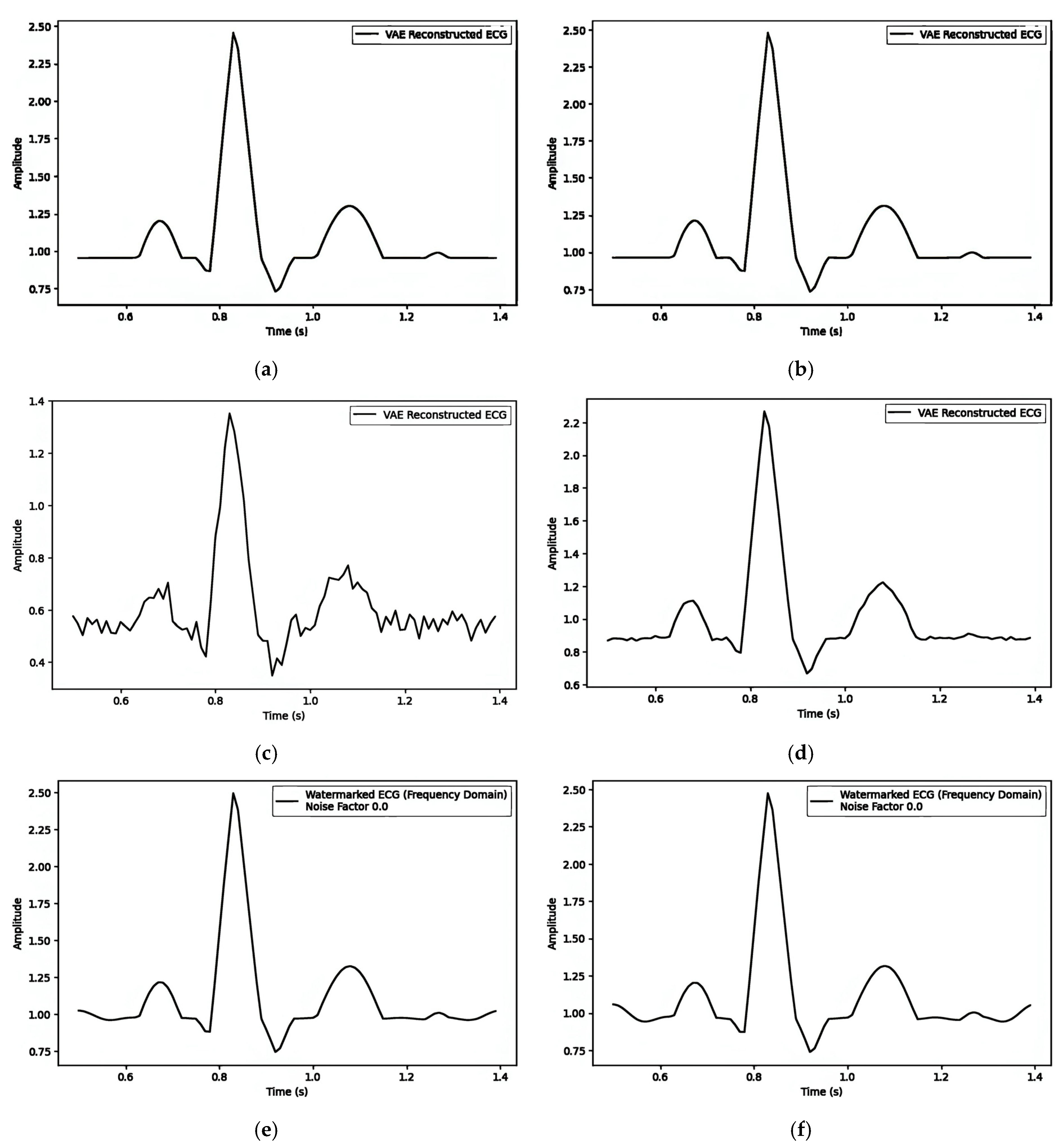
4.5.3. Embedding Watermark Through Frequency Domain
5. Conclusions
Author Contributions
Funding
Institutional Review Board Statement
Informed Consent Statement
Data Availability Statement
Conflicts of Interest
References
- Li, G.; Ma, X.; Wang, X.; Yue, H.; Li, J.; Liu, L.; Feng, X.; Xue, J. Optimizing deep neural networks on intelligent edge accelerators via flexible-rate filter pruning. J. Syst. Archit. 2022, 124, 102431. [Google Scholar] [CrossRef]
- Liu, L.; Ma, X.; Liu, H.; Li, G.; Liu, L. FlexPDA: A flexible programming framework for deep learning accelerators. J. Comput. Sci. Technol. 2022, 37, 1200–1220. [Google Scholar] [CrossRef]
- Li, G.; Ma, X.; Wang, X.; Liu, L.; Xue, J.; Feng, X. Fusion-catalyzed pruning for optimizing deep learning on intelligent edge devices. IEEE Trans. Comput. Aided Des. Integr. Circuits Syst. 2020, 39, 3614–3626. [Google Scholar] [CrossRef]
- Sanivarapu, P.V.; Rajesh, K.N.V.P.S.; Reddy, N.V.R.; Reddy, K.V.K.; Rao, P.V.R.; Reddy, A.S. Patient Data Hiding into ECG Signal Using Watermarking in Transform Domain. Phys. Eng. Sci. Med. 2020, 43, 213–226. [Google Scholar] [CrossRef]
- Kaur, S.; Singhal, R.; Farooq, O.; Ahuja, B.S. Digital Watermarking of ECG Data for Secure Wireless Communication. In Proceedings of the 2010 International Conference on Recent Trends in Information, Kerala, India, 12–13 March 2010; pp. 140–144. [Google Scholar] [CrossRef]
- Chen, S.-T.; Ye, R.-J.; Wu, T.-H.; Cheng, C.-W.; Zhan, P.-Y.; Chen, K.-M.; Zhong, W.-Y. Patient Confidential Data Hiding and Transmission System Using Amplitude Quantization in the Frequency Domain of ECG Signals. Sensors 2023, 23, 9199. [Google Scholar] [CrossRef]
- Khaldi, A.; Kafi, M.R.; Moad, M.S. Wrapping Based Curvelet Transform Approach for ECG Watermarking in Telemedicine Application. Biomed. Signal Process. Control 2022, 75, 103540. [Google Scholar] [CrossRef]
- Goyal, L.M.; Mittal, M.; Kaushik, R.; Verma, A.; Kaur, I.; Roy, S.; Kim, T.-H. Improved ECG Watermarking Technique Using Curvelet Transform. Sensors 2020, 20, 2941. [Google Scholar] [CrossRef]
- Engin, M.; Çıdam, O.; Engin, E.Z. Wavelet Transformation Based Watermarking Technique for Human Electrocardiogram (ECG). J. Med. Syst. 2005, 29, 589–594. [Google Scholar] [CrossRef]
- Huang, Y.; Niu, B.; Guan, H.; Zhang, S. Enhancing Image Watermarking with Adaptive Embedding Parameter and PSNR Guarantee. IEEE Trans. Multimed. 2019, 21, 2447–2460. [Google Scholar] [CrossRef]
- Kumar, S.; Rajpal, A.; Sharma, N.K.; Rajpal, S.; Nayyar, A.; Kumar, N. ROSEmark: Robust Semi-Blind ECG Watermarking Scheme Using SWT-DCT Framework. Digit. Signal Process. 2022, 129, 103648. [Google Scholar] [CrossRef]
- Jafari, F.; Tinati, M.A.; Mozaffari, B. A New Fetal ECG Extraction Method Using Its Skewness Value Which Lies in Specific Range. In Proceedings of the 2010 18th Iranian Conference on Electrical Engineering, Isfahan, Iran, 11–13 May 2010; pp. 30–34. [Google Scholar] [CrossRef]
- Priya, J.Y.; Suganya, R. Steganography Techniques for ECG Signals: A Survey. In Proceedings of the 2016 11th International Conference on Industrial and Information Systems (ICIIS), Roorkee, India, 3–4 December 2016; pp. 269–273. [Google Scholar] [CrossRef]
- Ibaida, A.; Khalil, I. Wavelet-Based ECG Steganography for Protecting Patient Confidential Information in Point-of-Care Systems. IEEE Trans. Biomed. Eng. 2013, 60, 3322–3330. [Google Scholar] [CrossRef]
- LeCun, Y.; Bengio, Y.; Hinton, G. Deep Learning. Nature 2015, 521, 436–444. [Google Scholar] [CrossRef] [PubMed]
- Annadurai, C.; Nelson, I.; Devi, K.N.; Manikandan, R.; Gandomi, A.H. Image Watermarking Based Data Hiding by Discrete Wavelet Transform Quantization Model with Convolutional Generative Adversarial Architectures. Appl. Sci. 2023, 13, 804. [Google Scholar] [CrossRef]
- Mincholé, A.; Rodríguez, B. Artificial Intelligence for the Electrocardiogram. Nat. Med. 2019, 25, 22–23. [Google Scholar] [CrossRef] [PubMed]
- Tamura, S.; Tateishi, M. Capabilities of a Four-Layered Feedforward Neural Network: Four Layers Versus Three. IEEE Trans. Neural Netw. 1997, 8, 251–255. [Google Scholar] [CrossRef]
- Rajpurkar, P.; Hannun, A.Y.; Haghpanahi, M.; Bourn, C.; Ng, A.Y. Cardiologist-Level Arrhythmia Detection with Convolutional Neural Networks. arXiv 2017, arXiv:1710.10121. [Google Scholar]
- Rashed-Al-Mahfuz, M.; Moni, M.A.; Lio, P.; Islam, S.M.S.; Berkovsky, S.; Khushi, M.; Quinn, J.M.W. Deep Convolutional Neural Networks Based ECG Beats Classification to Diagnose Cardiovascular Conditions. Biomed. Eng. Lett. 2021, 11, 147–162. [Google Scholar] [CrossRef]
- Singh, P.; Pradhan, G. A New ECG Denoising Framework Using Generative Adversarial Network. IEEE/ACM Trans. Comput. Biol. Bioinform. 2021, 18, 759–764. [Google Scholar] [CrossRef]
- Goodfellow, I.; Pouget-Abadie, J.; Mirza, M.; Xu, B.; Warde-Farley, D.; Ozair, S.; Courville, A.; Bengio, Y. Generative Adversarial Nets. In Proceedings of the 28th International Conference on Neural Information Processing Systems—Volume 2, Montreal, QC, Canada, 8–13 December 2014. [Google Scholar] [CrossRef]
- Kingma, D.P.; Welling, M. Auto-Encoding Variational Bayes. arXiv 2014, arXiv:1312.6114. [Google Scholar]
- Doersch, C. Tutorial on Variational Autoencoders. arXiv 2016, arXiv:1606.05908. [Google Scholar]
- Zhao, J.; Hou, X.; Pan, M.; Zhang, H. Attention-Based Generative Adversarial Network in Medical Imaging: A Narrative Review. Comput. Biol. Med. 2022, 149, 105948. [Google Scholar] [CrossRef] [PubMed]
- Hsu, C.-Y.; Chen, C.-C.; Liu, C.-Y.; Chen, S.-T.; Tu, S.-Y. Intelligent Healthcare System Using Mathematical Model and Simulated Annealing to Hide Patients Data in the Low-Frequency Amplitude of ECG Signals. Sensors 2022, 22, 8341. [Google Scholar] [CrossRef] [PubMed]
- Karthik, R. ECG Simulation Using MATLAB. Principle of Fourier Series; College of Engineering Guindy, Anna University: Chennai, India, 2006. [Google Scholar]
- Kubicek, J.; Penhaker, M.; Kahankova, R. Design of a Synthetic ECG Signal Based on the Fourier Series. In Proceedings of the 2014 International Conference on Advances in Computing Communications and Informatics (ICACCI), Delhi, India, 24–27 September 2014; pp. 1881–1885. [Google Scholar] [CrossRef]
- Verma, S.; Mehta, K.; Mehta, S.; Sharma, M. Watermarking of ECG Signals Using Wavelet Transform for Privacy Preservation. J. Biomed. Inform. 2020, 103, 103448. [Google Scholar]
- Vincent, P.; LaRochelle, H.; Bengio, Y.; Manzagol, P.-A. Extracting and composing robust features with denoising autoencoders. In Proceedings of the 25th international conference on Machine learning (ICML ’08), New York, NY, USA, 5 July 2008; pp. 1096–1103. [Google Scholar] [CrossRef]
- Giorgino, T. Computing and Visualizing Dynamic Time Warping Alignments in R: The dtw Package. J. Stat. Softw. 2009, 31, 1–24. [Google Scholar] [CrossRef]
- Chen, S.-Y.; Lin, S.-J.; Tsai, M.-C.; Tsai, M.-D.; Tang, Y.-J.; Chen, S.-T.; Wang, L.-H. Patient Confidential Information Transmission Using the Integration of PSO-based Biomedical Signal Steganography and Threshold-based Compression. J. Med. Biol. Eng. 2021, 41, 433–446. [Google Scholar] [CrossRef]
- Zhao, M.; Chen, S.-T.; Chen, T.-L.; Tu, S.-Y.; Yeh, C.-T.; Lin, F.-Y.; Lu, H.-C. Intelligent Healthcare System Using Patients Confidential Data Communication in Electrocardiogram Signals. Front. Aging Neurosci. 2022, 14, 870844. [Google Scholar] [CrossRef]


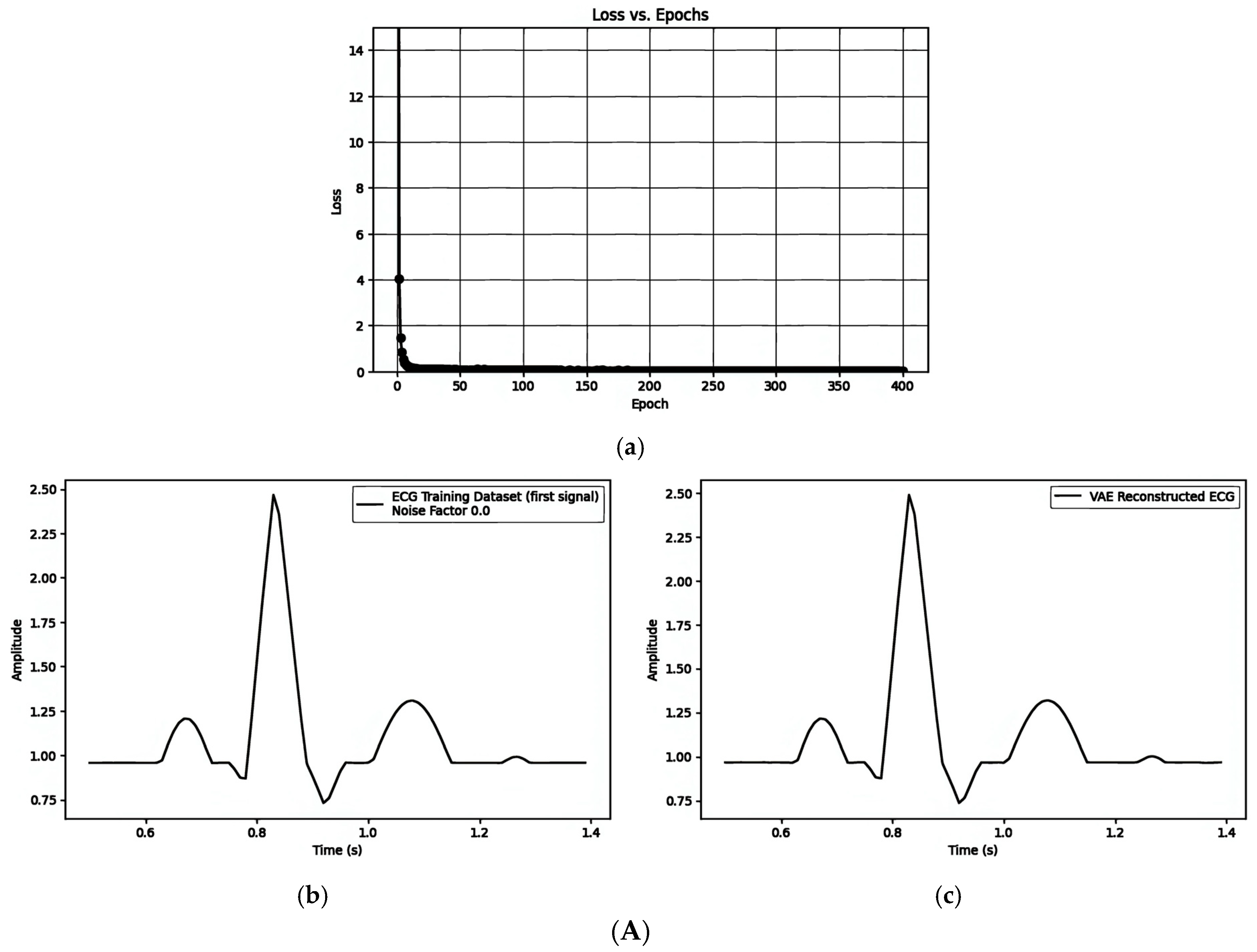
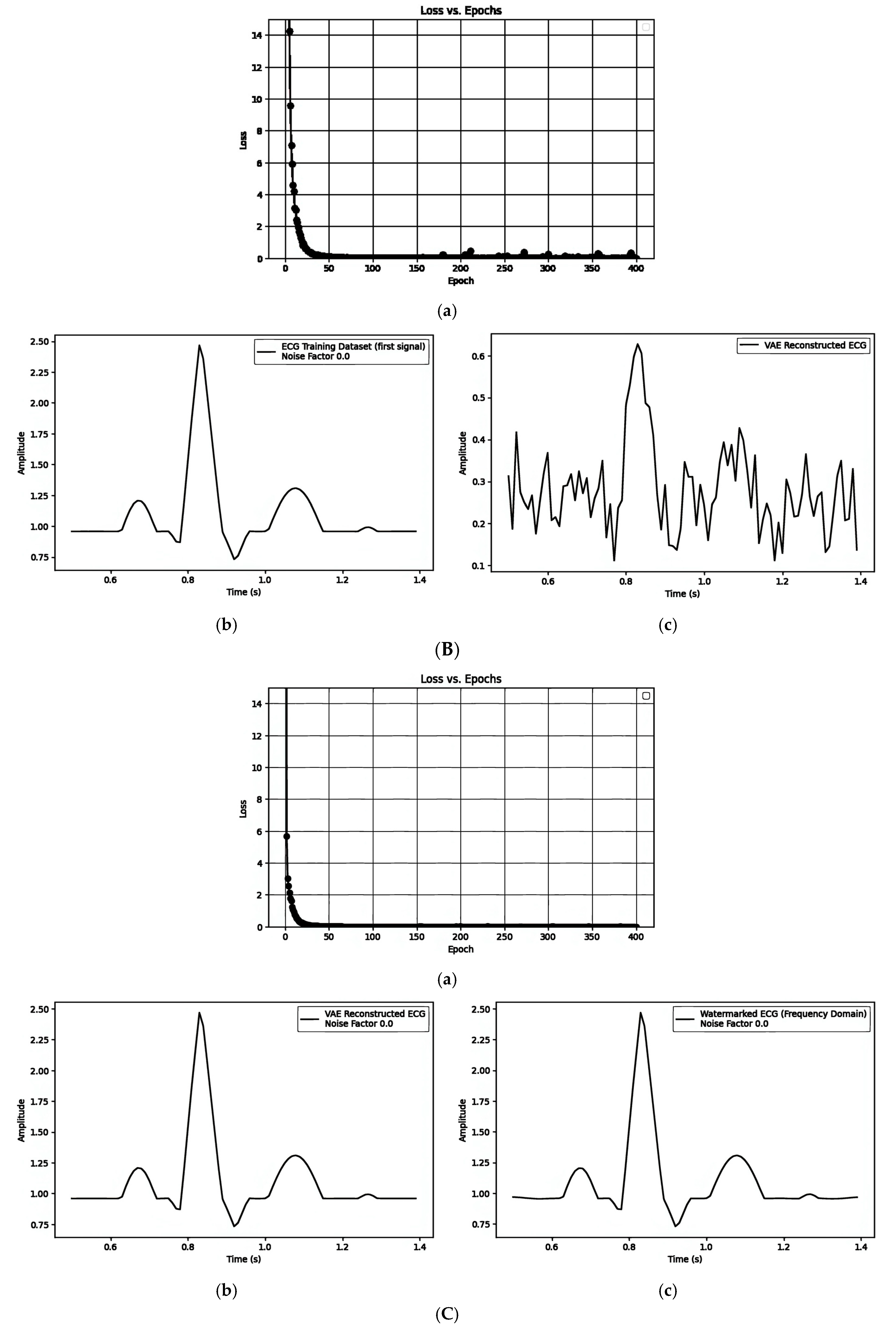
| Figure 7A(a–c)/Figure 7B(a–c)/Figure 7C(a–c) | ||||||
|---|---|---|---|---|---|---|
| Model Parameters | Data Parameters | |||||
| Input dimension | Latent dimension | Learning rate | Batch size | Training epochs | Noise factor | Watermark length |
| 90 | 20 | 0.001 | 32 | 400 | 0.0 | 10 |
| Watermarking Strategies | MSE | Comprison Figures | alpha |
|---|---|---|---|
| 1. Pre-Reconstruction Watermarking: Embedding the watermark in the mean () | 0.00025240 | Figure 7A(b) and Figure 7A(c) | 0.1 |
| 0.00002263 | Figure 5b and Figure 8a | 0.5 | |
| 0.00002474 | Figure 5b and Figure 8b | 0.9 | |
| 2. Pre-Reconstruction Watermarking: Embedding watermarks through the latent variable () | 0.71435501 | Figure 7B(b) and Figure 7B(c) | 0.1 |
| 0.25729716 | Figure 5b and Figure 8c | 0.5 | |
| 0.00806380 | Figure 5b and Figure 8d | 0.9 | |
| 3. Post-Reconstruction Watermarking: Embedding watermarks through the frequency domain | 0.00000679 | Figure 7C(b) and Figure 7C(c) | 0.1 |
| 0.00016975 | Figure 5b and Figure 8e | 0.5 | |
| 0.00055000 | Figure 5b and Figure 8f | 0.9 |
| Watermarking Strategies | MSE | Dimension of Latent Space |
|---|---|---|
| 1. Pre-Reconstruction Watermarking: Embedding the watermark in the mean () | 0.00002229 | 30 |
| 0.00002773 | 20 | |
| 0.00003235 | 10 | |
| 2. Pre-Reconstruction Watermarking: Embedding watermarks through the latent variable () | 0.00000756 | 30 |
| 0.00030506 | 20 | |
| 0.01020047 | 10 |
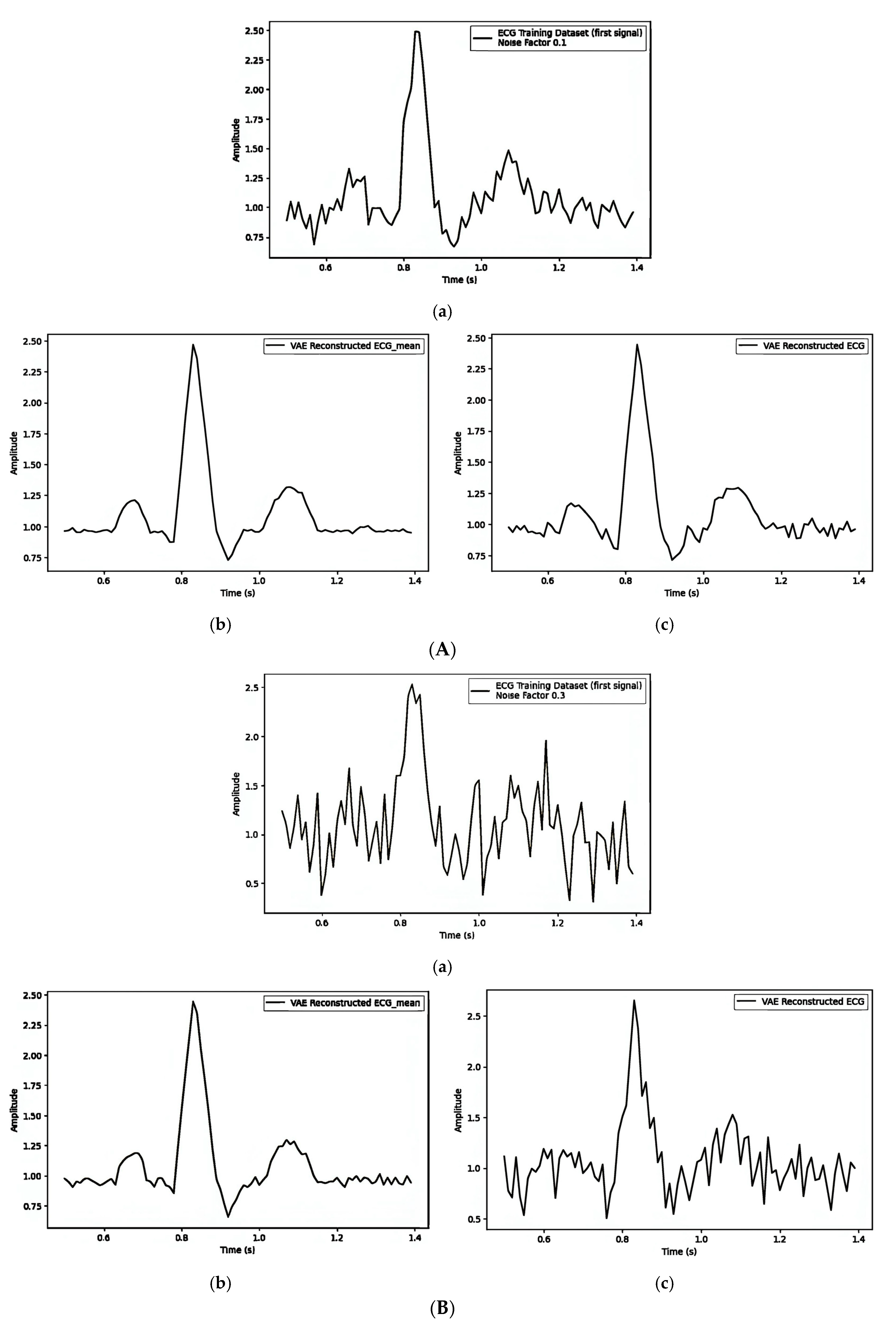
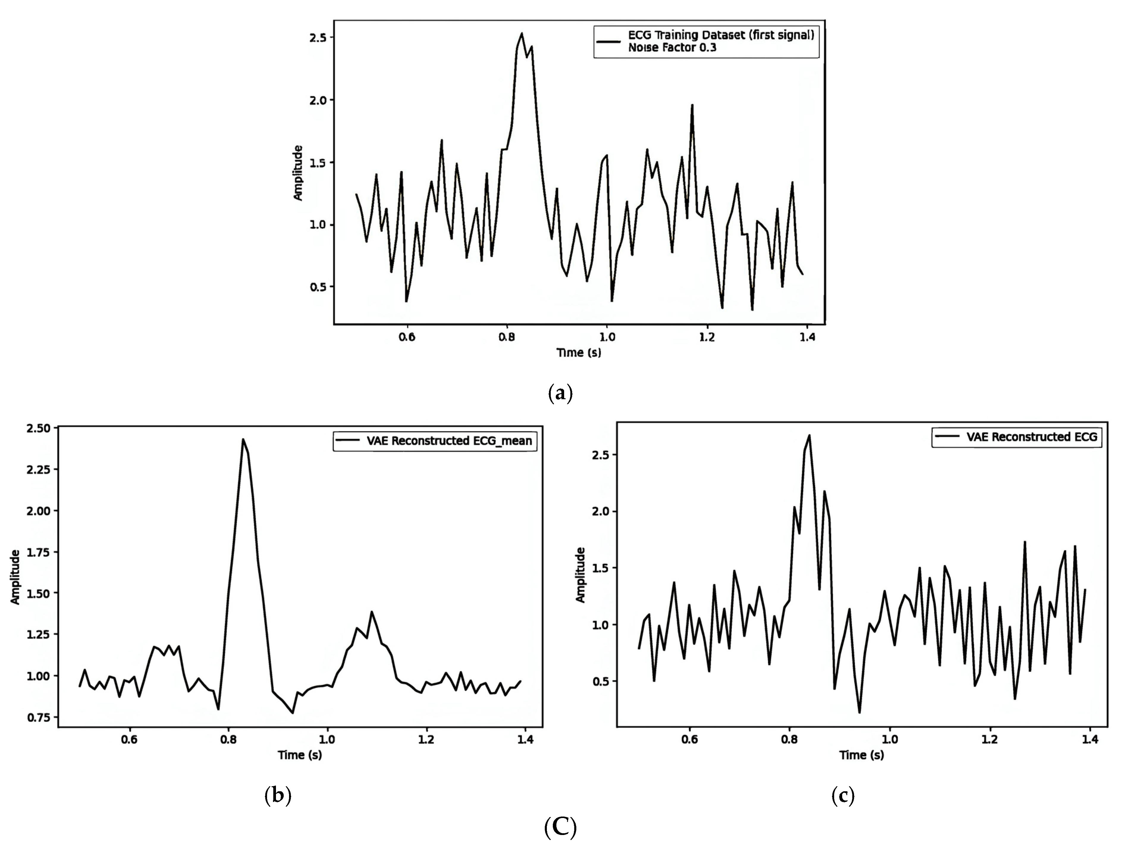
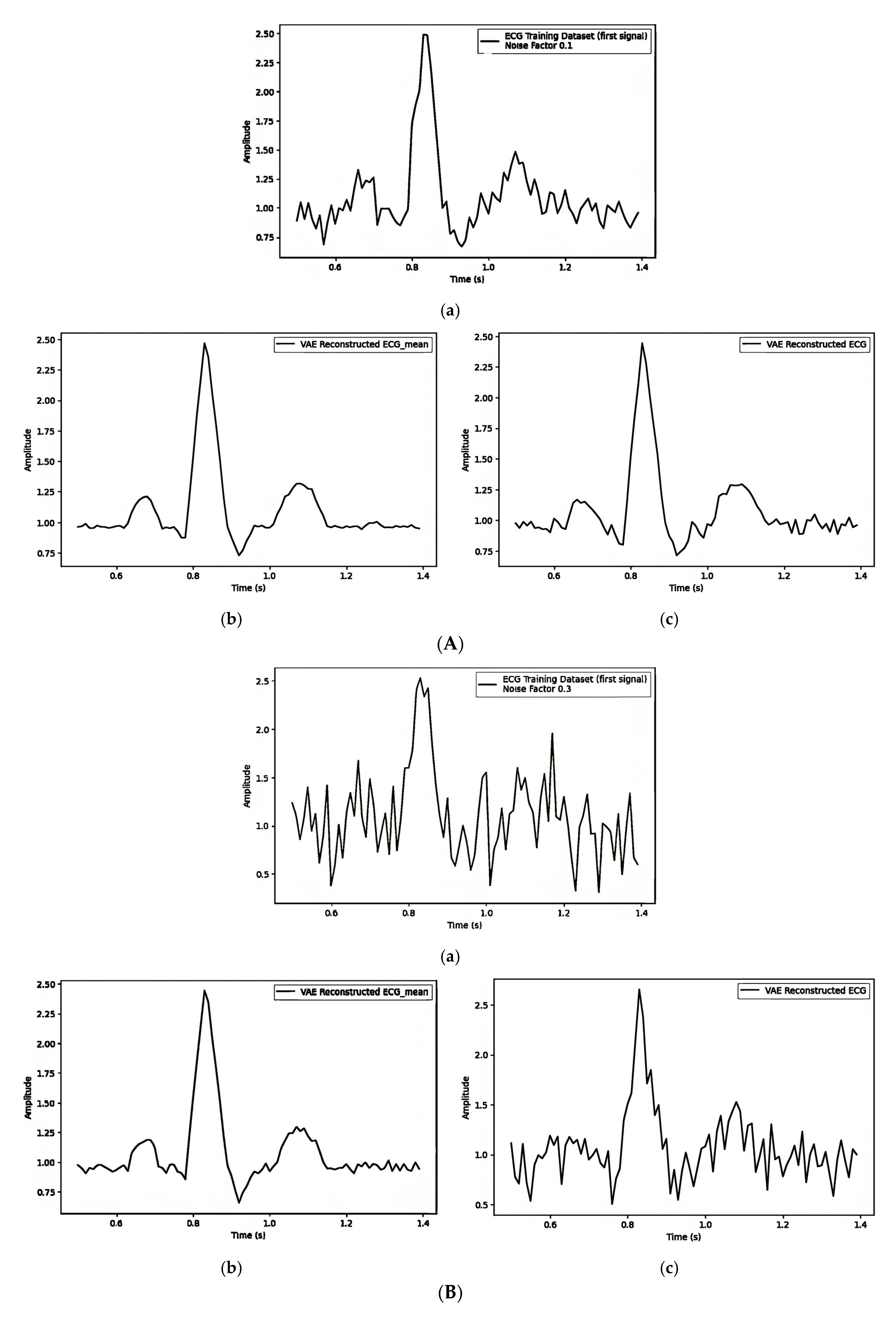
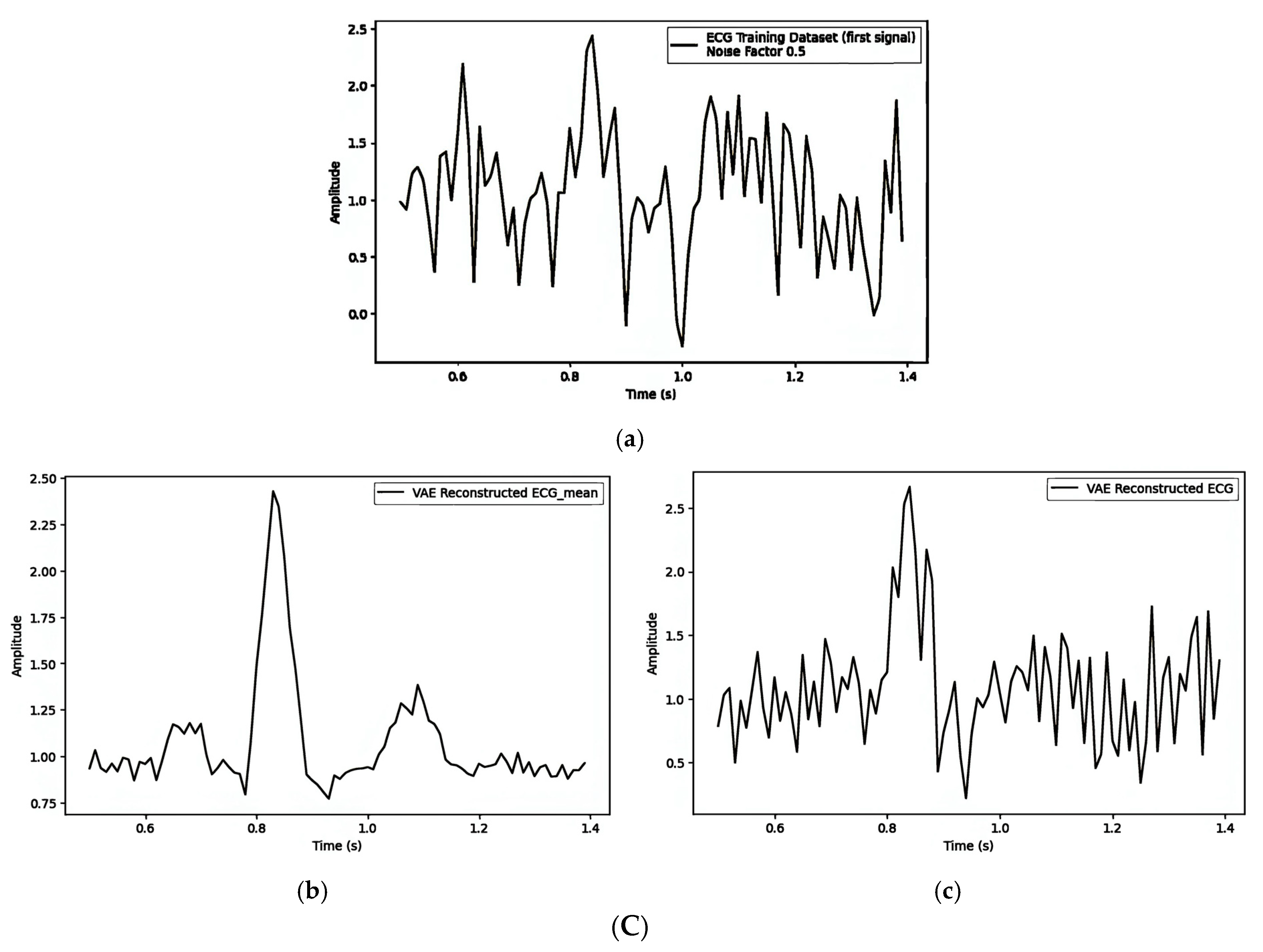
| Noise Factor | Figure 9A/Figure 9B/Figure 9C | |||||
|---|---|---|---|---|---|---|
| MSE | DTW | |||||
| (a) vs. (b) | (a) vs. (c) | (b) vs. (c) | (a) vs. (b) | (a) vs. (c) | (b) vs. (c) | |
| 0.1 | 0.0098 | 0.0122 | 0.0016 | 8.85 | 9.12 | 3.67 |
| 0.3 | 0.1033 | 0.1736 | 0.0494 | 23.37 | 24.04 | 17.42 |
| 0.5 | 0.2260 | 0.3738 | 0.1063 | 38.48 | 38.60 | 25.79 |
| Noise Factor | Figure 10A/Figure 10B/Figure 10C | |||||
|---|---|---|---|---|---|---|
| MSE | DTW | |||||
| (a) vs. (b) | (a) vs. (c) | (b) vs. (c) | (a) vs. (b) | (a) vs. (c) | (b) vs. (c) | |
| 0.1 | 0.0823 | 0.0969 | 0.0216 | 22.63 | 20.92 | 12.32 |
| 0.3 | 0.0918 | 0.1018 | 0.0102 | 23.76 | 21.92 | 9.06 |
| 0.5 | 0.2639 | 0.4514 | 0.1599 | 37.45 | 34.80 | 28.18 |
| Noise Factor | Figure 11A/Figure 11B/Figure 11C | |||||
|---|---|---|---|---|---|---|
| MSE | DTW | |||||
| (a) vs. (b) | (a) vs. (c) | (b) vs. (c) (b) vs. (d) (c) vs. (d) | (a) vs. (b) | (a) vs. (c) | (b) vs. (c) (b) vs. (d) (c) vs. (d) | |
| 0.1 | 0.00769329 | 0.00768736 | 0.00000606 | 7.36723554 | 7.38519794 | 0.35533977 |
| 0.00000849 | 0.31853223 | |||||
| 0.00000679 | 0.17227793 | |||||
| 0.3 | 0.09544947 | 0.09547500 | 0.00000714 | 22.89780141 | 22.87669791 | 0.38388956 |
| 0.00001911 | 0.52939296 | |||||
| 0.00000679 | 0.20855498 | |||||
| 0.5 | 0.22180541 | 0.22261526 | 0.00001820 | 37.97530274 | 37.92291443 | 0.58136564 |
| 0.00002480 | 0.67344922 | |||||
| 0.00000679 | 0.22654438 | |||||
| Data ID | Reference [32] (Time Domain) | Reference [33] (DWT Domain) | Proposed Method (Time Domain) | |||
|---|---|---|---|---|---|---|
| SNR | BER (%) | SNR | BER (%) | SNR | BER (%) | |
| 1 | 51.7 | 23.2 | 38.4 | 25.1 | 50.4 | 0 |
| 2 | 68.3 | 21.1 | 32.7 | 24.3 | 52.3 | 0 |
| 3 | 60.9 | 23.7 | 34.2 | 23.8 | 50.6 | 0 |
| 4 | 55.7 | 24.5 | 37.4 | 24.6 | 51.3 | 0 |
| 5 | 38.4 | 25.3 | 32.5 | 25.3 | 48.5 | 0 |
| 6 | 29.2 | 20.7 | 26.9 | 23.7 | 42.6 | 0 |
| 7 | 63.6 | 22.8 | 26.7 | 26.2 | 53.2 | 0 |
| 8 | 40.3 | 24.1 | 41.9 | 24.5 | 48.5 | 0 |
Disclaimer/Publisher’s Note: The statements, opinions and data contained in all publications are solely those of the individual author(s) and contributor(s) and not of MDPI and/or the editor(s). MDPI and/or the editor(s) disclaim responsibility for any injury to people or property resulting from any ideas, methods, instructions or products referred to in the content. |
© 2025 by the authors. Licensee MDPI, Basel, Switzerland. This article is an open access article distributed under the terms and conditions of the Creative Commons Attribution (CC BY) license (https://creativecommons.org/licenses/by/4.0/).
Share and Cite
Hsu, C.-Y.; Chang, C.-Y.; Chen, Y.-C.; Wu, J.; Chen, S.-T. ECG Sensor Design Assessment with Variational Autoencoder-Based Digital Watermarking. Sensors 2025, 25, 2321. https://doi.org/10.3390/s25072321
Hsu C-Y, Chang C-Y, Chen Y-C, Wu J, Chen S-T. ECG Sensor Design Assessment with Variational Autoencoder-Based Digital Watermarking. Sensors. 2025; 25(7):2321. https://doi.org/10.3390/s25072321
Chicago/Turabian StyleHsu, Chih-Yu, Chih-Yin Chang, Yin-Chi Chen, Jasper Wu, and Shuo-Tsung Chen. 2025. "ECG Sensor Design Assessment with Variational Autoencoder-Based Digital Watermarking" Sensors 25, no. 7: 2321. https://doi.org/10.3390/s25072321
APA StyleHsu, C.-Y., Chang, C.-Y., Chen, Y.-C., Wu, J., & Chen, S.-T. (2025). ECG Sensor Design Assessment with Variational Autoencoder-Based Digital Watermarking. Sensors, 25(7), 2321. https://doi.org/10.3390/s25072321