

Modeling Debris Flow Events in the Rio Inferno Watershed (Italy) Through UAV-Based Geomorphological Survey and Rainfall Data Analysis


Abstract
1. Introduction
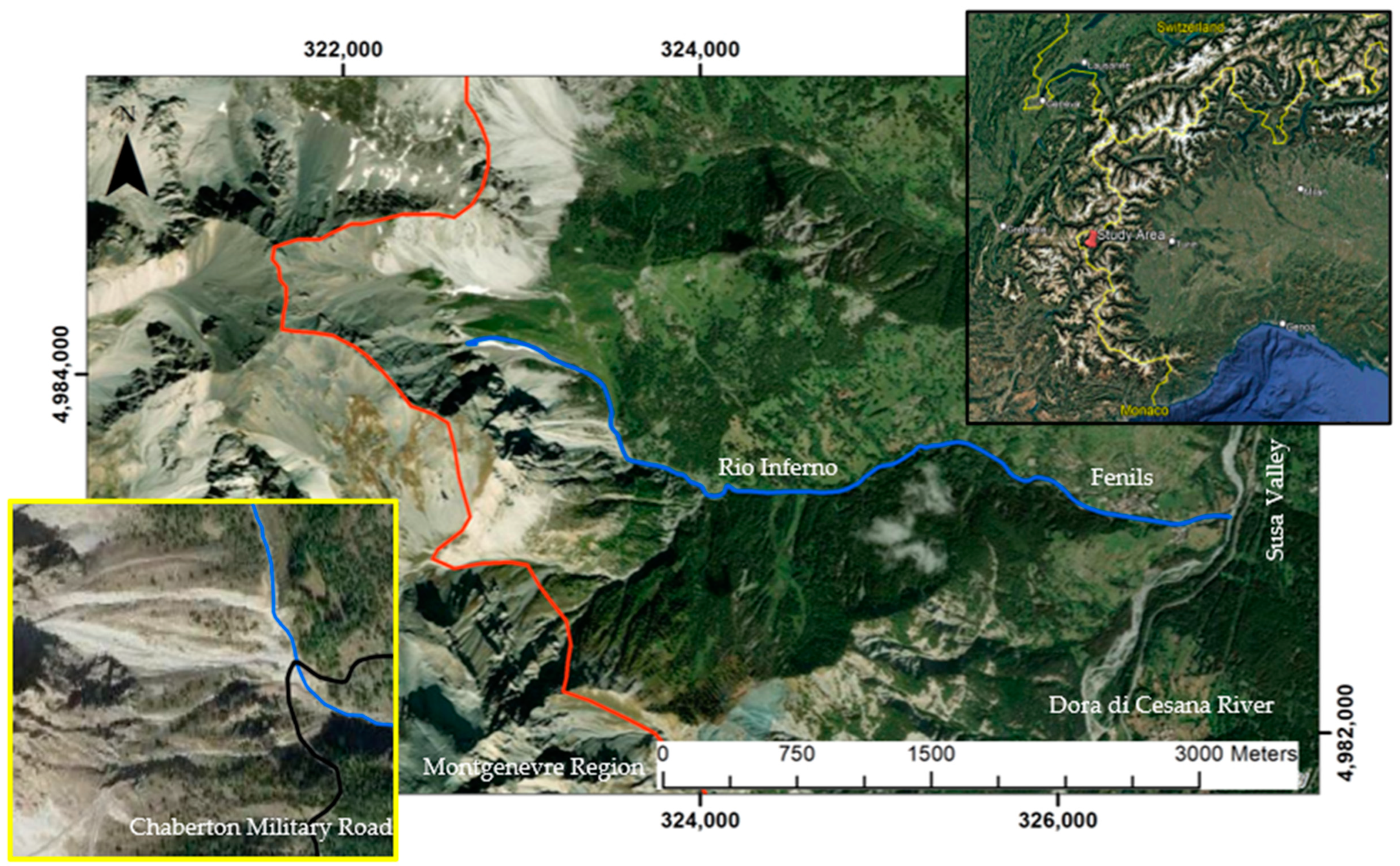
2. Case Study
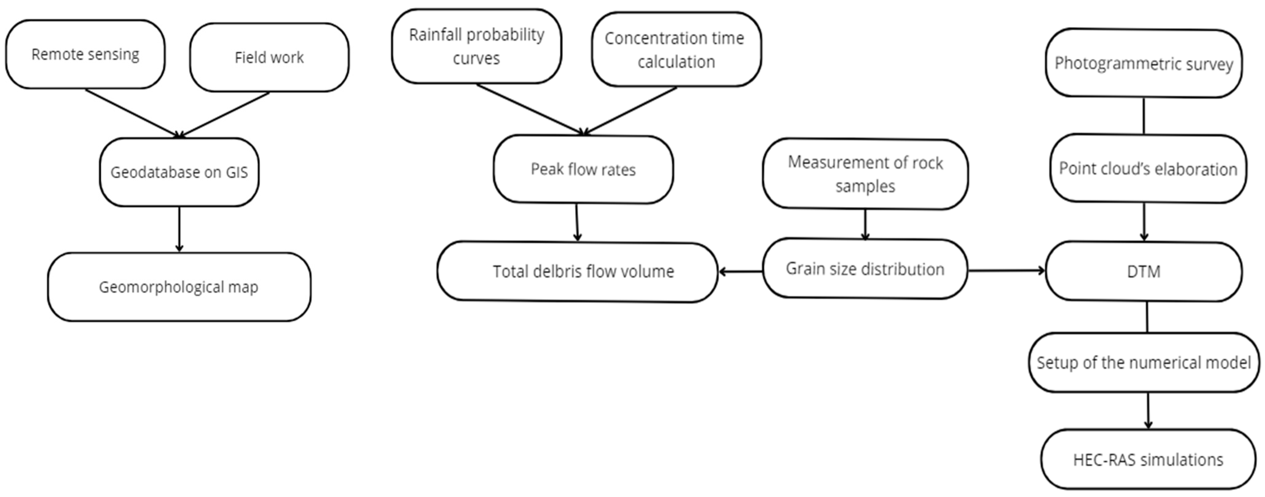
3. Materials and Methods
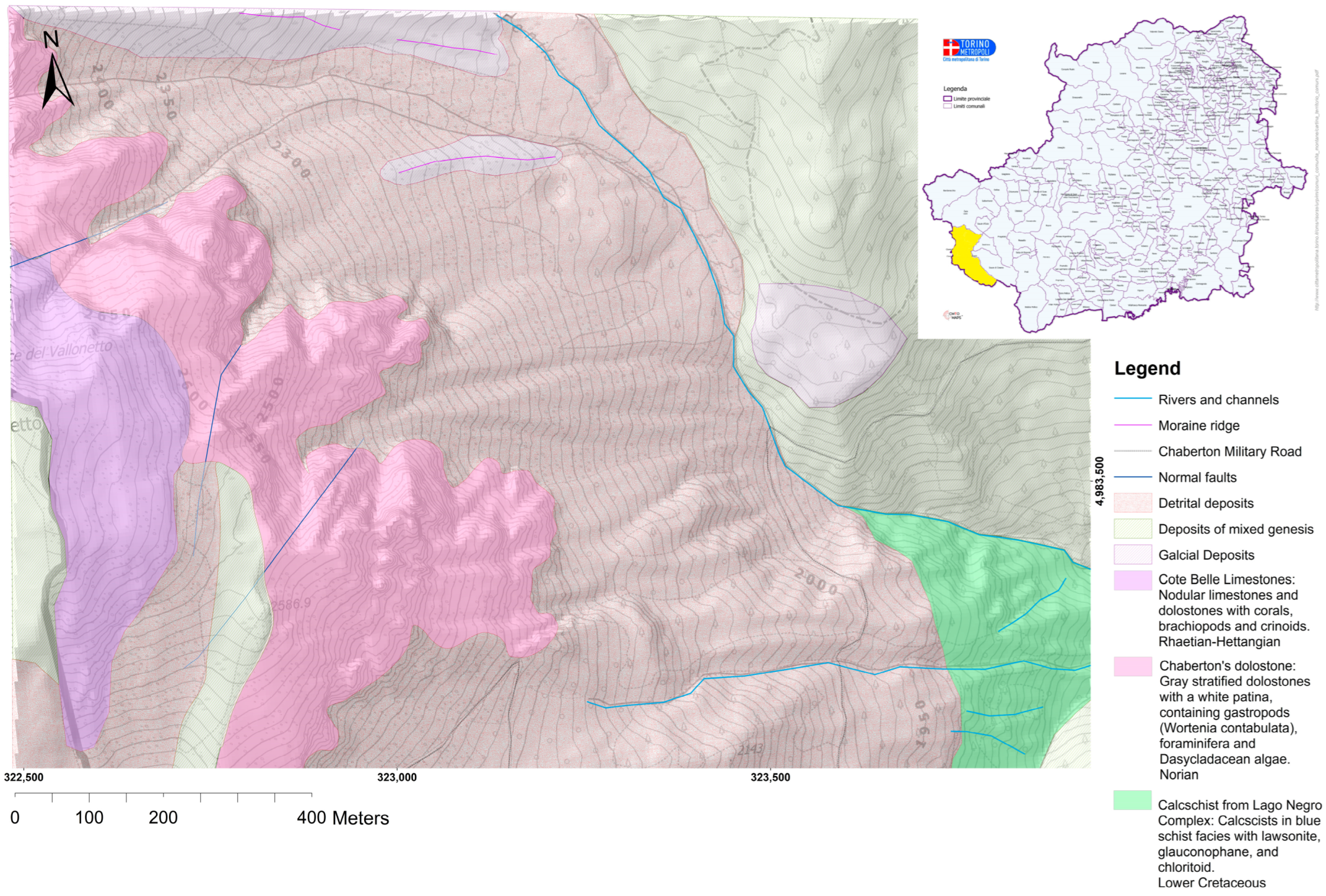
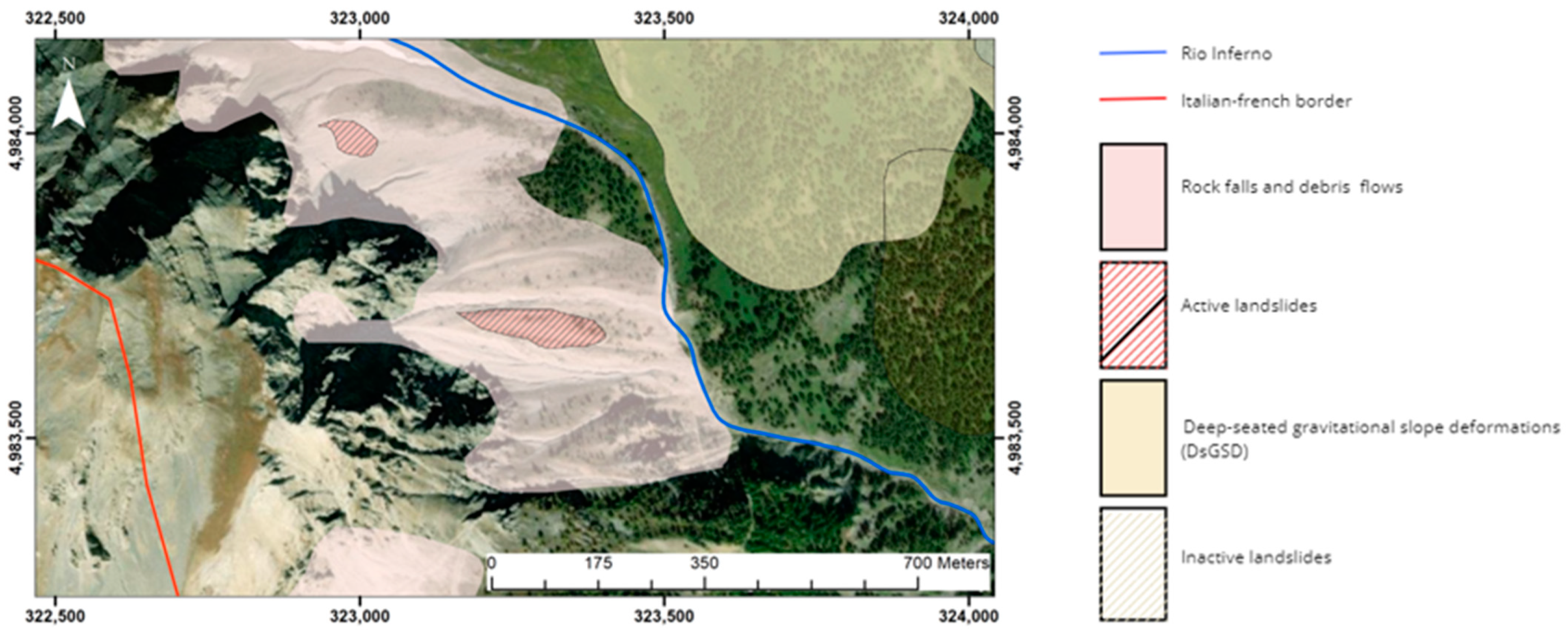
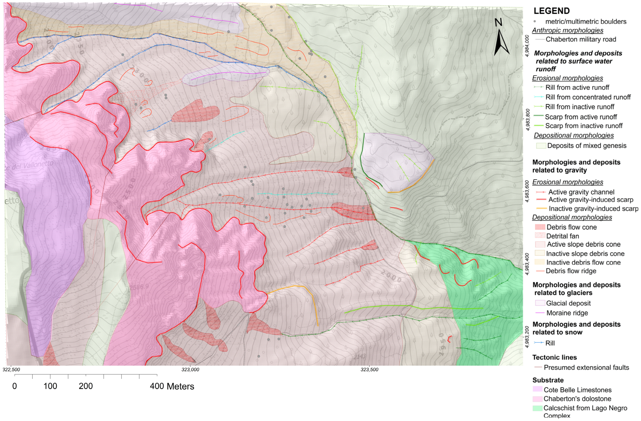
3.1. Geomorphological Map of the Rio Inferno Watershed
- Observed landforms → classified into erosional and depositional forms;
- Morphogenetic agents → categorized as gravity, surface water, ice, snow, and anthropogenic;
- State of activity → active or inactive.
3.2. Flow Volume and Maximum Flow Rate
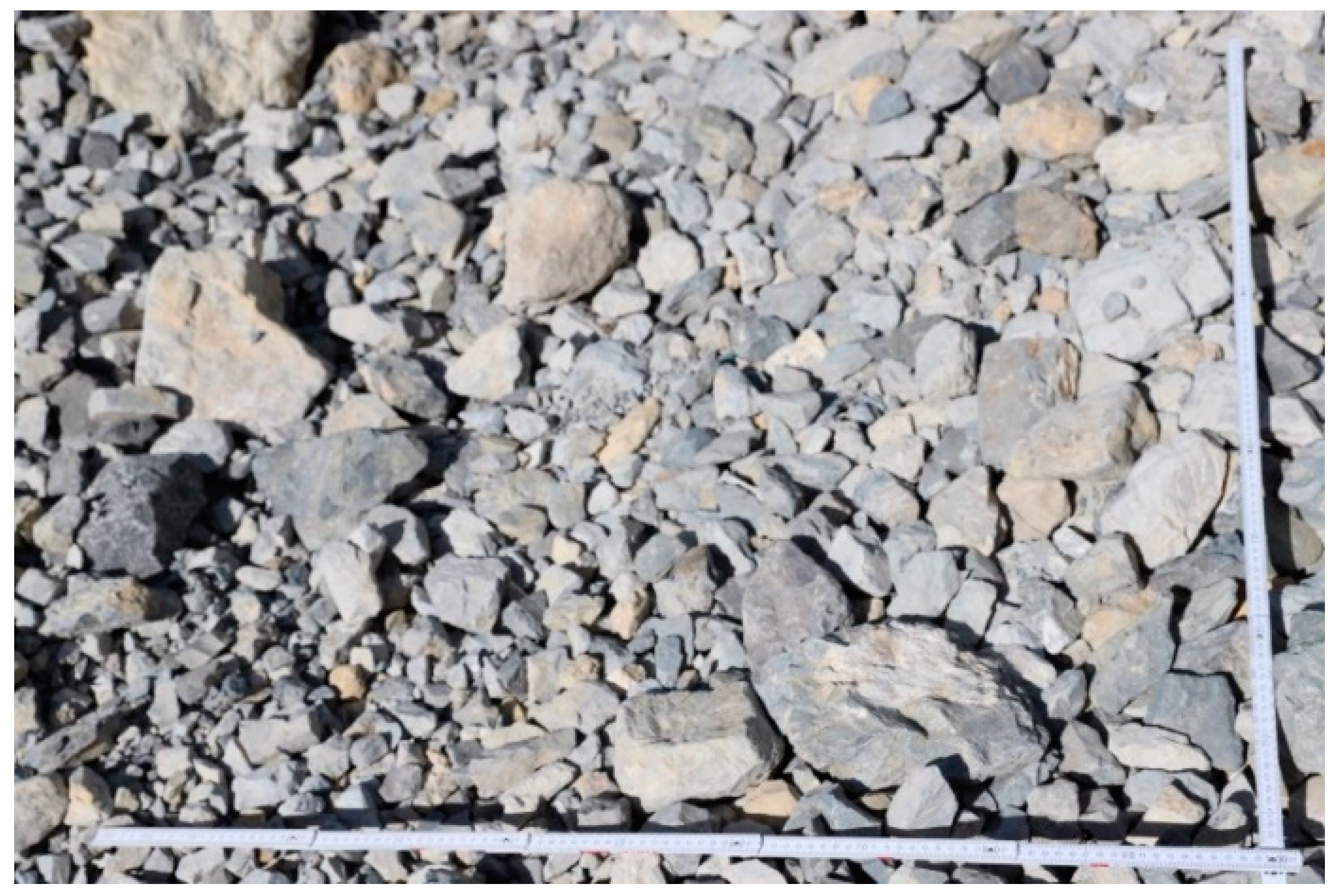
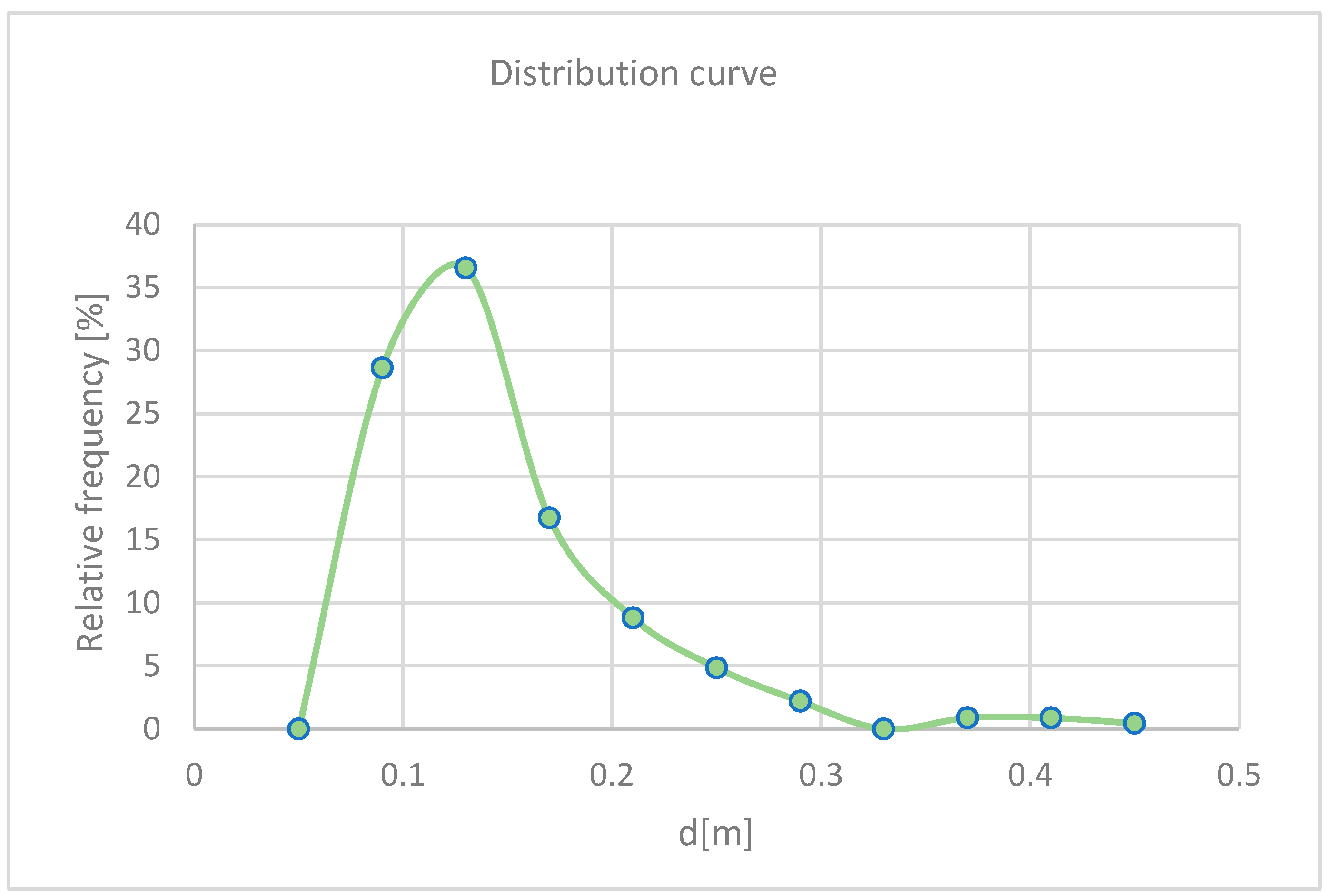
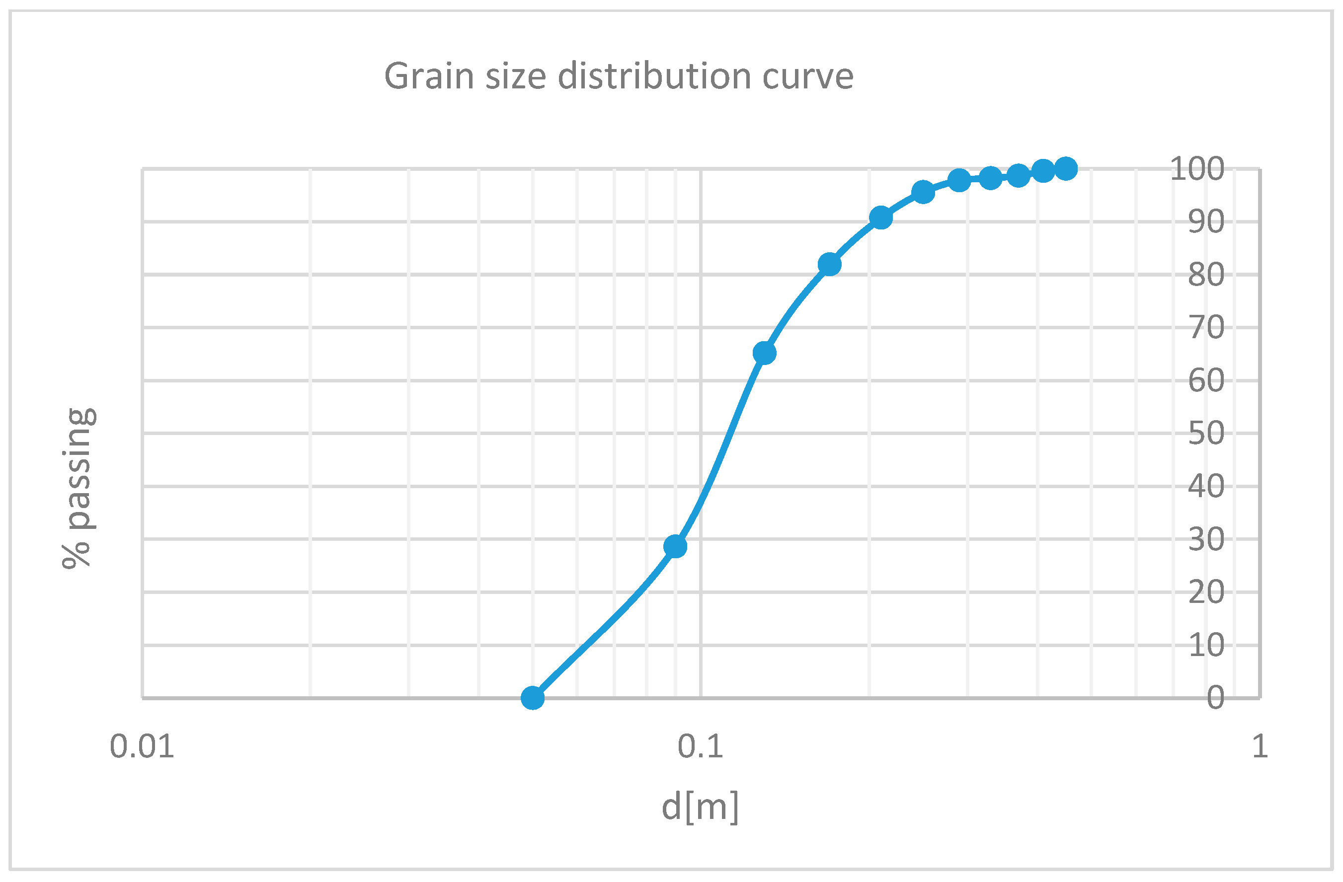
3.3. Grain Size Distribution
3.4. The Debris Flow Numerical Model
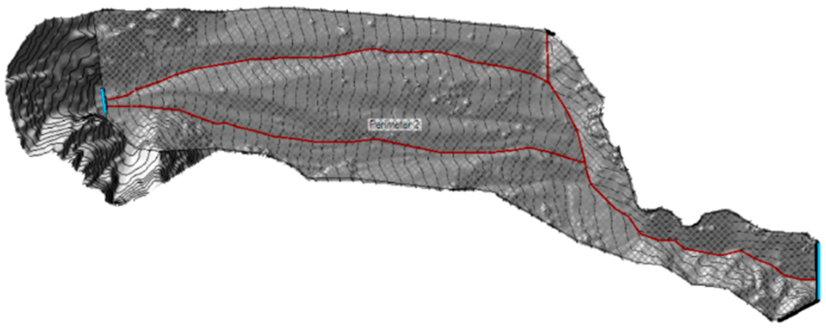
- A model perimeter within which the simulation is carried out.
- Boundary condition lines: an inflow line located upstream of the study area and an outflow line located downstream. These define the start and end points of the model.
- Breaklines, one for each primary channel identified in the simulation perimeter. These lines are necessary to guide the software in determining the directions in which the flow will develop.
- Flow data, including the flood hydrograph.
3.5. Photogrammetric Survey and DTM
4. Results
4.1. Geomorphological Survey and Mapping of the Rio Inferno Watershed
4.2. Computation of Input Parameters
4.3. Construction of the Grain Size Distribution
4.4. Set up of the Debris Flow Numerical Model
5. Discussion
6. Conclusions
Author Contributions
Funding
Institutional Review Board Statement
Informed Consent Statement
Data Availability Statement
Acknowledgments
Conflicts of Interest
References
- Bello, S.; Perna, M.G.; Consalvo, A.; Brozzetti, F.; Galli, P.; Cirillo, D.; Andrenacci, C.; Tangari, A.C.; Carducci, A.; Menichetti, M.; et al. Coupling rare earth element analyses and high-resolution topography along fault scarps to investigate past earthquakes: A case study from the Southern Apennines (Italy). Geosphere 2023, 19, 1348–1371. [Google Scholar] [CrossRef]
- Perks, M.T.; Russell, A.J.; Large, A.R.G. Technical Note: Advances in flash flood monitoring using unmanned aerial vehicles (UAVs). Hydrol. Earth Syst. Sc. 2016, 20, 4005–4015. [Google Scholar] [CrossRef]
- Cirillo, D.; Zappa, M.; Tangari, A.C.; Brozzetti, F.; Ietto, F. Rockfall Analysis from UAV-Based Photogrammetry and 3D Models of a Cliff Area. Drones 2024, 8, 31. [Google Scholar] [CrossRef]
- Sun, J.W.; Yuan, G.Q.; Song, L.Y.; Zhang, H.W. Unmanned Aerial Vehicles (UAVs) in Landslide Investigation and Monitoring: A Review. Drones 2024, 8, 30. [Google Scholar] [CrossRef]
- Román, A.; Tovar-Sánchez, A.; Roque-Atienza, D.; Huertas, I.E.; Caballero, I.; Fraile-Nuez, E.; Navarro, G. Unmanned aerial vehicles (UAVs) as a tool for hazard assessment: The 2021 eruption of Cumbre Vieja volcano, La Palma Island (Spain). Sci. Total Env. 2022, 843, 157092. [Google Scholar] [CrossRef]
- Amodio, A.M.; Corrado, G.; Gallo, I.G.; Gioia, D.; Schiattarella, M.; Vitale, V.; Robustelli, G. Three-Dimensional Rockslide Analysis Using Unmanned Aerial Vehicle and LiDAR: The Castrocucco Case Study, Southern Italy. Remote Sens. 2024, 16, 2235. [Google Scholar] [CrossRef]
- Zemp, M.; Frey, H.; Gärtner-Roer, I.; Nussbaumer, S.U.; Hoelzle, M.; Paul, F.; Haeberli, W.; Denzinger, F.; Ahlstrøm, A.P.; Anderson, B.; et al. Historically unprecedented global glacier decline in the early 21st century. J. Glaciol. 2015, 61, 745–762. [Google Scholar] [CrossRef]
- National Academies of Sciences, Engineering, and Medicine. Attribution of Extreme Weather Events in the Context of Climate Change; The National Academies Press: Washington, DC, USA, 2016. [Google Scholar] [CrossRef]
- Roe, G.H.; Baker, M.B.; Herla, F. Centennial glacier retreat as categorical evidence of regional climate change. Nat. Geosci. 2017, 10, 95–99. [Google Scholar] [CrossRef]
- Gariano, S.L.; Guzzetti, F. Landslides in a changing climate. Earth Sci. Rev. 2016, 162, 227–252. [Google Scholar] [CrossRef]
- Cruden, D.M.; Varnes, D.J. Landslide types and processes. In Landslides Investigation and Mitigation: Transportation Research Board; Turner, A.K., Scuster, R.L., Eds.; Special Report 247; US National Research Council: Washington, DC, USA, 1996; pp. 36–75. [Google Scholar]
- Iverson, R.M. The Physics of Debris Flows. Rev. Geophys. 1997, 35, 245–296. [Google Scholar] [CrossRef]
- Hungr, O.; Leroueil, S.; Picarelli, L. The Varnes classification of landslide types, an update. Landslides 2014, 11, 167–194. [Google Scholar]
- Costa, J.E. Physical geomorphology of debris flows. In Developments and Applications in Geomorphology; Costa, J.E., Fleischer, P.J., Eds.; Springer: Berlin/Heidelberg, Germany, 1984; pp. 268–317. [Google Scholar]
- Frank, F.; McArdell, B.W.; Huggel, C.; Vieli, A. The importance of entrainment and bulking on debris flow runout modeling: Examples from the Swiss Alps. Nat. Hazard. Earth Sys. 2015, 15, 2569–2583. [Google Scholar] [CrossRef]
- Mantovani FPatusto, A.; Silvano, S. Definition of the elements at risk and mitigation measures of the Cancia debris flow (Dolomites, northeastern Italy). Engineering Geology for 144 developing Countries. In Proceedings of the 9th Congress of the International Association for Engineering Geology and the Environment, Durban, South Africa, 16–20 September 2002; pp. 16–20. [Google Scholar]
- Berti, M.; Simoni, A. Experimental evidences and numerical modelling of debris flow Initiated by Channel runoff. Landslides 2005, 2, 171–182. [Google Scholar]
- Jakob, M.; Hungr, O. Debris-Flow Hazards and Related Phenomena; Praxis Publishing Ldt.: Berlin/Heidelberg, Germany, 2005. [Google Scholar]
- ISPRA—IdroGEO. Inventario Dei Fenomeni Franosi d’Italia (IFFI). Available online: https://idrogeo.isprambiente.it/app/iffi (accessed on 26 July 2024).
- Polaris (Popolazione a Rischio da Frana e da Inondazione in Italia). Available online: https://polaris.irpi.cnr.it/report/last-report/ (accessed on 23 July 2024).
- Turbessi, L. Caratterizzazione Geomorfologica e Geotecnica del Bacino del Rio Inferno (Cesana Torinese Fraz.Fenils). Master’s Thesis, Department of Earth Science, Università degli studi di Torino, Turin, Italy, 2024. [Google Scholar]
- ISPRA. Dissesto Idrogeologico in Italia: Pericolosità e Indicatori di Rischio. Rapporti 356/2021; ISPRA: Roma, Italy, 2021. [Google Scholar]
- Vagnon, F.; Ferrero, A.M.; Pirulli, M.; Segalini, A. Theoretical and experimental study for the optimization of fexible barriers to restrain debris fows. Geoing. Ambient. E Mineraria 2015, 145, 29–35. [Google Scholar]
- Vagnon, F.; Ferrero, A.M.; Alejano, L.R. Reliability-based design for debris flow barriers. Landslides 2020, 17, 49–59. [Google Scholar] [CrossRef]
- Vagnon, F.; Kurilla, L.J.; Clusaz, A.; Pirulli, M.; Fubelli, G. Investigation and numerical simulation of debris flow events in Rochefort basin (Aosta Valley—NW Italian Alps) combining detailed geomorphological analyses and modern technologies. Bull. Eng. Geol. Environ. 2022, 81, 378. [Google Scholar] [CrossRef]
- Vagnon, F. Design of active debris fow mitigation measures: A comprehensive analysis of existing impact models. Landslides 2020, 17, 313–333. [Google Scholar] [CrossRef]
- Hec Ras User Manual. Available online: https://www.hec.usace.army.mil/confluence/rasdocs/rasum/latest (accessed on 26 April 2024).
- ARPA Piemonte. Atlante Delle Piogge Intense. Available online: https://webgis.arpa.piemonte.it/agportal/apps/webappviewer/index.html?id=378e0fcb7ddd4565ba836c07dd1c4c9b (accessed on 24 April 2024).
- Polino, R.; Borghi, A.; Carraro, F.; Dela Pierre, F.; Fioraso, G.; Giardino, M. Note illustrative della Carta Geologica d’Italia alla scala 1:50.000. Foglio 132-152-153 “Bardonecchia”. Servizio Geologico d’Italia. 2002. Available online: https://www.isprambiente.gov.it/Media/carg/153_BARDONECCHIA/Foglio.html (accessed on 23 March 2024).
- Fioraso, G.; Mosca, P. Note illustrative della carta geologica di Italia alla scala 1:50:000- Foglio 171 “Cesana Torinese”. Ispra-Serv.Geol.It. 2014. Available online: https://www.isprambiente.gov.it/Media/carg/171_CESANA_TORINESE/Foglio.html (accessed on 23 March 2024).
- ARPA Piemonte. Sistema Informativo Frane in Piemonte (SIFRAP). Available online: https://www.arpa.piemonte.it/dato/sistema-informativo-frane-piemonte-sifrap (accessed on 25 July 2024).
- Geoportale Regione Piemonte. Ortofoto RGB AGEA. 2018. Available online: https://www.geoportale.piemonte.it/geonetwork/srv/ita/catalog.search#/home (accessed on 8 November 2021).
- Campobasso, C.; Carton, A.; Chelli, A.; D’Orefice, M.; Dramis, F.; Graciotti, R.; Guida, D.; Pambianchi, G.; Peduto, F.; Pellegrini, L. Aggiornamento ed integrazioni delle Linee Guida della Carta Geomorfologica d'Italia alla scala 1: 50.000-Progetto CARG: Modifiche ed integrazioni al Quaderno n. 4/1994. I Quad. Ser. III Del Serv. Geol. D'italia (SGI). 2018, 13, 1–95. [Google Scholar]
- QGIS Development Team. QGIS Geographic Information System. Open Source Geospatial Foundation Project. 2002. Available online: http://qgis.osgeo.org (accessed on 27 March 2024).
- Gumbel, E.J. The Return Period of Flood Flows. Ann. Math. Stat. 1941, 12, 163–190. [Google Scholar]
- Kirpich, Z.P. Concentration time of small agricultural watersheds. Civ. Eng. 1940, 10, 362. [Google Scholar]
- Chow, V.E. Open-Channel Hydraulics; McGraw-Hill: New York, NY, USA, 1959. [Google Scholar]
- Kuichling, E. The relation between the Rainfall and the Discharge of Sewers in Populous Disctricts. Trans. Am. Soc. Civ. Eng. 1889, 20, 1–56. [Google Scholar]
- Benini, G. Sistemazioni Idraulico Forestali. In Collana: Scienze Forestali e Ambientali; UTET: Torino, Italy, 1990; EAN 9788802043401; ISBN 88-02-04340-X. [Google Scholar]
- Armanini, A. Colate di detriti; Geol. Institute of the Italian Republic and Canton Ticino: Rome, Italy, 1996; Work Report. [Google Scholar]
- Takahashi, T. Mechanical Characteristics of Debris Flow. J. Hydraul. Div. 1978, 104, 1153–1169. [Google Scholar] [CrossRef]
- Coussot, P.; Meunier, M. Recognition, classification and mechanical description of debris flows. Earth Sci. Rev. 1996, 40, 209–227. [Google Scholar]
- Ferreira, T.; Rasband, W. ImageJ User Guide; Version 1.54k; National Institutes of Health: Bethesda, MD, USA, 2011; Available online: https://imagej.net/ij/index.html (accessed on 5 July 2024).
- Yang, J.; Townsend, R.D.; Daneshfar, B. Applying the HEC-RAS model and GIS techniques in river network floodplain delineation. Can. J. Civ. Eng. 2006, 33, 19–28. [Google Scholar]
- Khattak, M.S.; Anwar, F.; Saeed, T.U.; Sharif, M.; Sheraz, K.; Ahmed, A. Floodplain mapping using HEC-RAS and ArcGIS: A case study of Kabul River. Arab. J. Sci. Eng. 2016, 41, 1375–1390. [Google Scholar]
- Yılmaz, K.; Dinçer, A.E.; Kalpakcı, V.; Öztürk, Ş. Debris flow modelling and hazard assessment for a glacier area: A case study in Barsem, Tajikistan. Nat. Hazards 2023, 115, 2577–2601. [Google Scholar] [CrossRef]
- Ekaso, D.; Nex, F.; Kerle, N. Accuracy assessment of real-time kinematics (RTK) measurements on unmanned aerial vehicles (UAV) for direct geo-referencing. Geo Spat. Inf. Sci. 2020, 23, 165–181. [Google Scholar] [CrossRef]
- Martínez-Carricondo, P.; Agüera-Vega, F.; Carvajal-Ramírez, F. Accuracy assessment of RTK/PPK UAV-photogrammetry projects using differential corrections from multiple GNSS fixed base stations. Geocarto Int. 2023, 38, 2197507. [Google Scholar] [CrossRef]
- 3DF Zephyr Free, Version 7.531; Computer Software. Available online: https://www.3dflow.net/3df-zephyr-free/ (accessed on 3 September 2024).
- Hartley, R.; Zisserman, A. Multiple View Geometry in Computer Vision; Cambridge University Press: Cambridge, UK, 2003; ISBN 0-521-54051-8. [Google Scholar]
- Cloud Compare, Version 2.13.2; GPL Software, 2024. Available online: http://www.cloudcompare.org/ (accessed on 3 September 2024).
- Fell, R. Landslide risk assessment and acceptable risk. Can. Geotechn. J. 1994, 31, 261–272. [Google Scholar]
- Hungr, O. Dynamics of Rock Avalanches and Other Types of Mass Movements. Ph.D. Thesis, University of Alberta, Edmonton, AB, Canada, 1981. [Google Scholar]


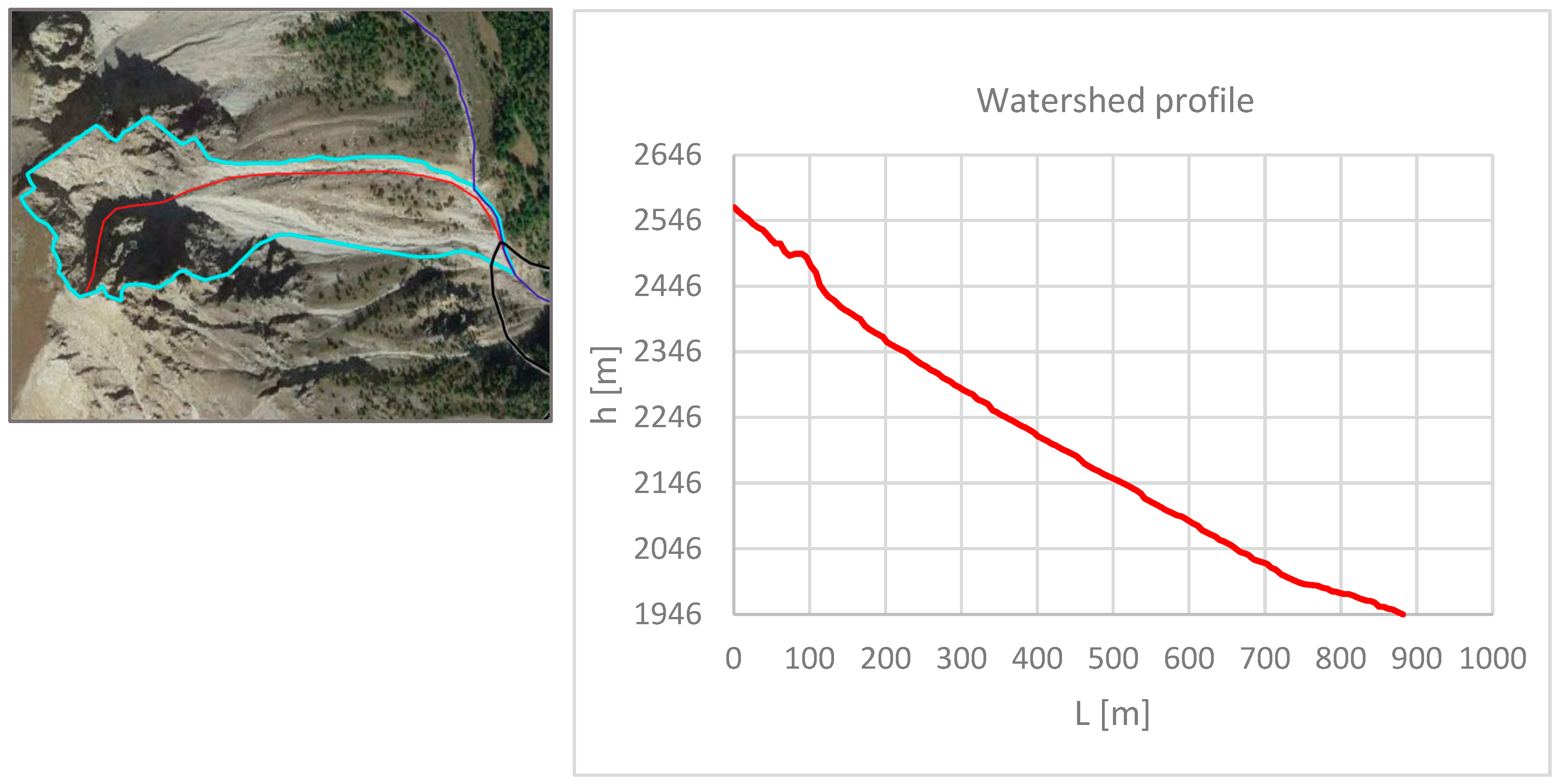
| L [m] | 881.77 |
| S (Δh/L) | 0.70 |
| tc Kirpich—Equation (2) [min] | |
| tc Chow—Equation (3) [min] |
| RP (Years) | QW (m3/s) [Equation (4)] | Qtot RM (m3/s) [Equation (4)] | Qtot VM (m3/s) [Equation (7)] |
|---|---|---|---|
| 20 | 3.01 | 10.03 | 30.08 |
| 50 | 3.54 | 11.79 | 35.36 |
| 100 | 3.93 | 13.11 | 39.33 |
| 200 | 4.33 | 14.43 | 43.28 |
| Vw (m3) | Vsolid (m3) | Vflow (m3) | Conc. |
|---|---|---|---|
| 757.93 | 1768.50 | 2526.42 | 70% |
| 891.00 | 2078.99 | 2969.98 | 70% |
| 991.12 | 2312.62 | 3303.74 | 70% |
| 1090.55 | 2544.62 | 3635.17 | 70% |
Disclaimer/Publisher’s Note: The statements, opinions and data contained in all publications are solely those of the individual author(s) and contributor(s) and not of MDPI and/or the editor(s). MDPI and/or the editor(s) disclaim responsibility for any injury to people or property resulting from any ideas, methods, instructions or products referred to in the content. |
© 2025 by the authors. Licensee MDPI, Basel, Switzerland. This article is an open access article distributed under the terms and conditions of the Creative Commons Attribution (CC BY) license (https://creativecommons.org/licenses/by/4.0/).
Share and Cite
Turbessi, L.; Taboni, B.; Umili, G.; Fubelli, G.; Ferrero, A.M. Modeling Debris Flow Events in the Rio Inferno Watershed (Italy) Through UAV-Based Geomorphological Survey and Rainfall Data Analysis. Sensors 2025, 25, 1980. https://doi.org/10.3390/s25071980
Turbessi L, Taboni B, Umili G, Fubelli G, Ferrero AM. Modeling Debris Flow Events in the Rio Inferno Watershed (Italy) Through UAV-Based Geomorphological Survey and Rainfall Data Analysis. Sensors. 2025; 25(7):1980. https://doi.org/10.3390/s25071980
Chicago/Turabian StyleTurbessi, Laura, Battista Taboni, Gessica Umili, Giandomenico Fubelli, and Anna Maria Ferrero. 2025. "Modeling Debris Flow Events in the Rio Inferno Watershed (Italy) Through UAV-Based Geomorphological Survey and Rainfall Data Analysis" Sensors 25, no. 7: 1980. https://doi.org/10.3390/s25071980
APA StyleTurbessi, L., Taboni, B., Umili, G., Fubelli, G., & Ferrero, A. M. (2025). Modeling Debris Flow Events in the Rio Inferno Watershed (Italy) Through UAV-Based Geomorphological Survey and Rainfall Data Analysis. Sensors, 25(7), 1980. https://doi.org/10.3390/s25071980