
A Method for Constructing a Loss Function for Multi-Scale Object Detection Networks


Abstract
1. Introduction
- A new method for constructing a loss function is proposed. By establishing a prediction probability function (PPF) related to the size of the label box, and substituting the label box size into the prediction probability functions of different feature layers, the probabilities of the target object being predicted by different feature layers can be obtained. The weights of anchor points for each sample in the classification loss function are then calculated based on these probability values, thereby constructing the classification loss. In the text, this loss function is referred to as the Predictive Probability Loss (PP-Loss).
- A statistical analysis was conducted on the prediction results of various common object detection networks with pyramid structures to determine the range of object sizes to which each feature layer is most sensitive. Based on this analysis, reasonable parameters for the prediction probability function were determined.
2. Related Work
2.1. Feature Pyramid Network in Target Detection Network
2.2. The Evolution of the YOLO Network Architecture
2.3. The Evolution of Loss Functions
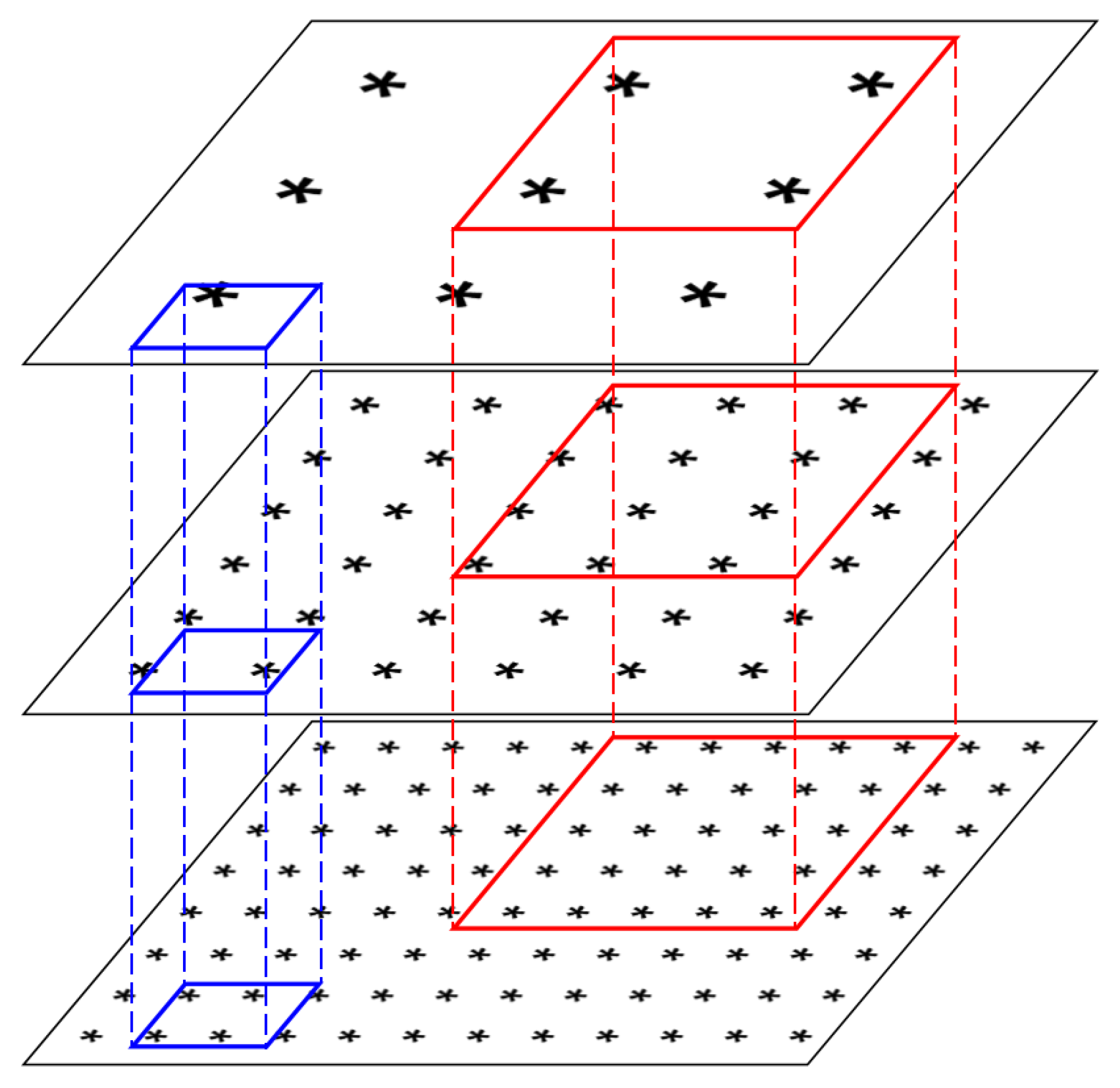
3. Methods
3.1. The Design of the Loss Function
3.2. The Definition of the Predictive Probability Function
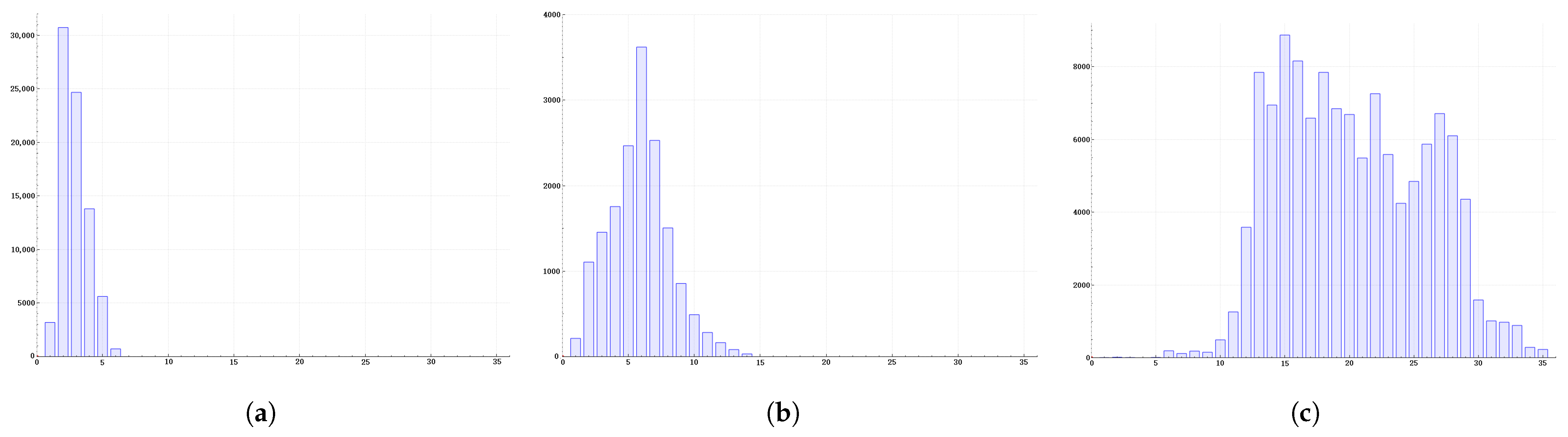
3.3. The Determination of Parameters
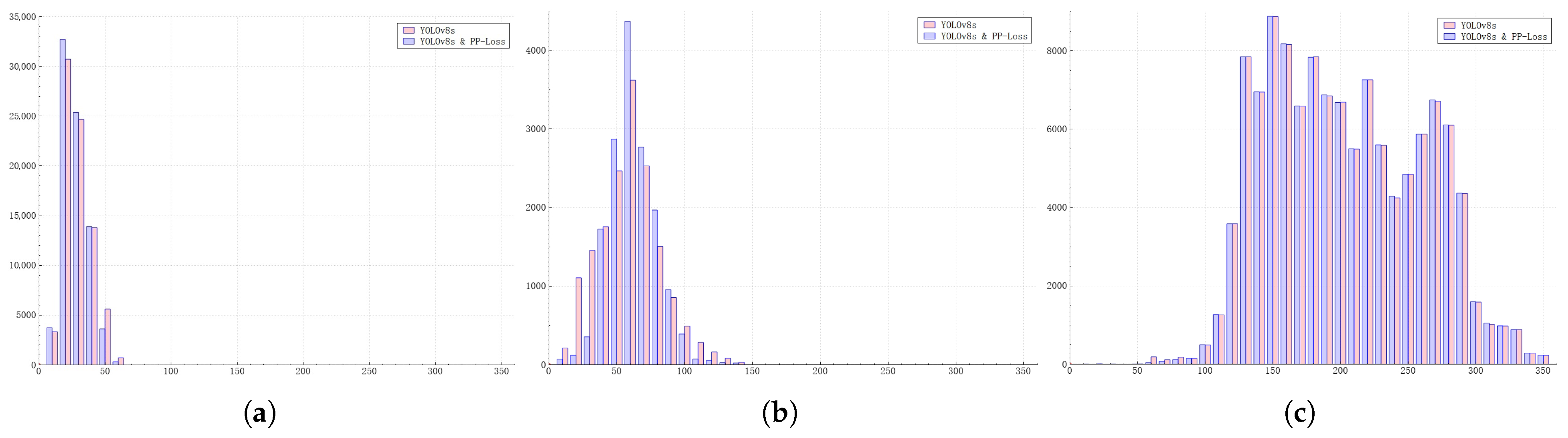
4. Results
4.1. Comparative Experiment
4.2. The Influence of Standard Deviation
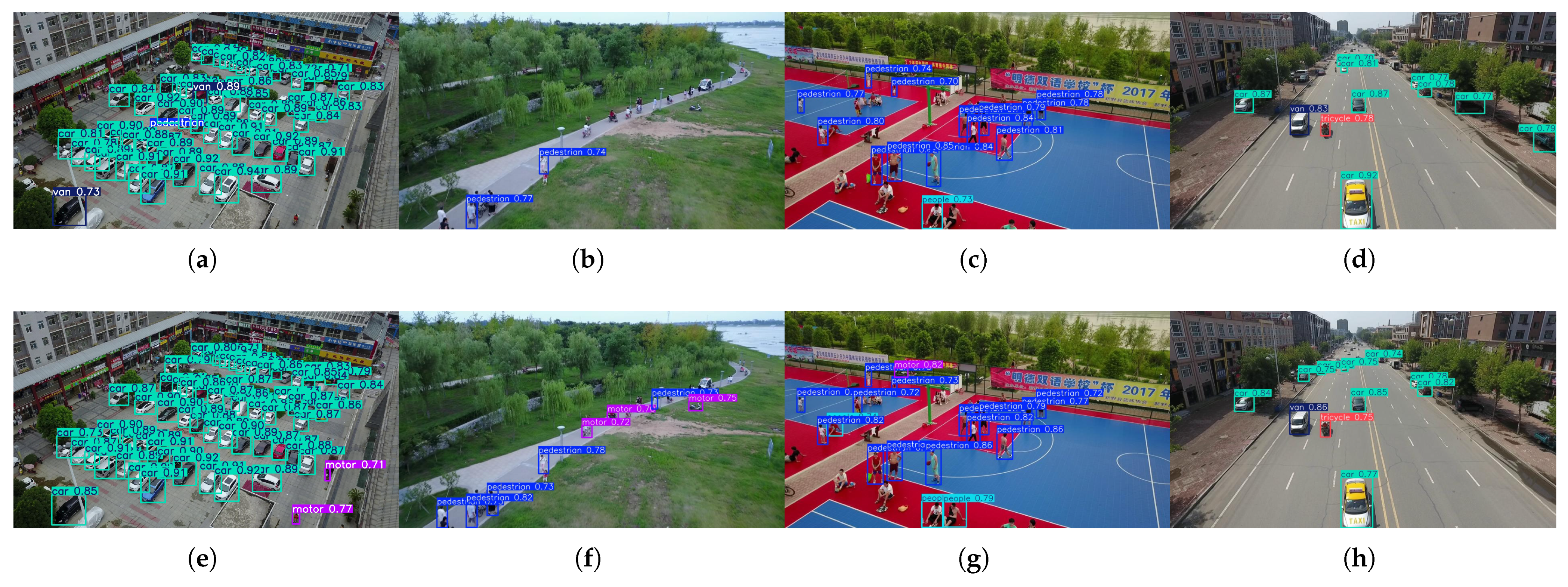
4.3. Comparison of the Detection Results
5. Discussion
6. Conclusions
Author Contributions
Funding
Institutional Review Board Statement
Informed Consent Statement
Data Availability Statement
Conflicts of Interest
Abbreviations
| PPF | Prediction Probability Function |
| PP-Loss | Prediction Probability Loss |
References
- Lin, T.-Y.; Dollár, P.; Girshick, R.; He, H.; Hariharan, B.; Belongiem, S. Feature Pyramid Networks for Object Detection. In Proceedings of the IEEE Conference on Computer Vision and Pattern Recognition (CVPR), Honolulu, HI, USA, 21–26 July 2017; pp. 2117–2125. [Google Scholar]
- Liu, S.; Qi, L.; Qin, H.; Shi, J.; Jia, J. Path Aggregation Network for Instance Segmentation. In Proceedings of the IEEE Conference on Computer Vision and Pattern Recognition (CVPR), Salt Lake City, UT, USA, 18–23 June 2018; pp. 8759–8768. [Google Scholar]
- Ghiasi, G.; Lin, T.Y.; Le, Q.V. NAS-FPN: Learning Scalable Feature Pyramid Architecture for Object Detection. In Proceedings of the IEEE Conference on Computer Vision and Pattern Recognition (CVPR), Long Beach, CA, USA, 15–20 June 2019; pp. 7036–7045. [Google Scholar]
- Xu, H.; Yao, L.; Zhang, W.; Liang, X.; Li, Z. Auto-FPN: Automatic Network Architecture Adaptation for Object Detection Beyond Classification. In Proceedings of the IEEE International Conference on Computer Vision (ICCV), Seoul, Republic of Korea, 27 October–2 November 2019; pp. 6649–6658. [Google Scholar]
- Tan, M.; Pang, R.; Le, Q.V. EfficientDet: Scalable and Efficient Object Detection. In Proceedings of the IEEE Conference on Computer Vision and Pattern Recognition (CVPR), Seattle, WA, USA, 13–19 June 2020; pp. 10781–10790. [Google Scholar]
- Lin, T.Y.; Goyal, P.; Girshick, R.; He, K.; Dollár, P. Focal Loss for Dense Object Detection. In Proceedings of the IEEE International Conference on Computer Vision (ICCV), Venice, Italy, 22–29 October 2017; pp. 2980–2988. [Google Scholar]
- Tian, Z.; Shen, C.; Chen, H.; He, T. FCOS: Fully Convolutional One-Stage Object Detection. In Proceedings of the IEEE International Conference on Computer Vision (ICCV), Seoul, Republic of Korea, 27 October–2 November 2019; pp. 9627–9636. [Google Scholar]
- Liu, W.; Anguelov, D.; Erhan, D.; Szegedy, C.; Reed, S.; Fu, C.Y.; Berg, A.C. SSD: Single Shot MultiBox Detector. In Proceedings of the European Conference on Computer Vision (ECCV), Amsterdam, The Netherlands, 11–14 October 2016; pp. 21–37. [Google Scholar]
- Redmon, J.; Divvala, S.; Girshick, R.; Farhadi, A. You Only Look Once: Unified, Real-Time Object Detection. In Proceedings of the IEEE Conference on Computer Vision and Pattern Recognition (CVPR), Las Vegas, NV, USA, 27–30 June 2016. [Google Scholar]
- Redmon, J.; Farhadi, A. YOLO9000: Better, Faster, Stronger. In Proceedings of the IEEE Conference on Computer Vision and Pattern Recognition (CVPR), Venice, Italy, 22–29 October 2017. [Google Scholar]
- Redmon, J.; Farhadi, A. YOLOv3: An Incremental Improvement. arXiv 2018, arXiv:1804.02767. [Google Scholar]
- Bochkovskiy, A.; Wang, C.-Y.; Liao, H.-Y.M. YOLOv4: Optimal Speed and Accuracy of Object Detection. arXiv 2020, arXiv:2004.10934. [Google Scholar]
- Ultralytics: YOLOv5. 2020. Available online: https://github.com/ultralytics/yolov5 (accessed on 10 January 2023.).
- Wang, C.-Y.; Bochkovskiy, A.; Liao, H.-Y.M. YOLOv7: Trainable Bag-of-Freebies Sets New State-of-the-Art for Real-Time Object Detectors. arXiv 2022, arXiv:2207.02696. [Google Scholar]
- Varghese, R.; Sambath, M. YOLOv8: A Novel Object Detection Algorithm with Enhanced Performance and Robustness. In Proceedings of the International Conference on Advances in Data Engineering and Intelligent Computing Systems (ADICS), Chennai, India, 18–19 April 2024. [Google Scholar]
- Tan, M.; Le, Q. EfficientNet: Rethinking Model Scaling for Convolutional Neural Networks. In Proceedings of the International Conference on Machine Learning (ICML), Long Beach, CA, USA, 10–15 June 2019; pp. 6105–6114. [Google Scholar]
- Zhou, X.; Wang, D.; Krähenbühl, P. Objects as Points. arXiv 2019, arXiv:1904.07850. [Google Scholar]
- He, K.; Zhang, X.; Ren, S.; Sun, J. Spatial Pyramid Pooling in Deep Convolutional Networks for Visual Recognition. IEEE Trans. Pattern Anal. Mach. Intell. 2015, 37, 1094–1916. [Google Scholar] [CrossRef] [PubMed]
- Wang, C.Y.; Liao, H.Y.M.; Wu, Y.H.; Chen, P.Y.; Hsieh, J.W.; Yeh, I.H. CSPNet: A New Backbone that can Enhance Learning Capability of CNN. In Proceedings of the IEEE/CVF Conference on Computer Vision and Pattern Recognition Workshops (CVPRW), Seattle, WA, USA, 14–19 June 2020; pp. 390–391. [Google Scholar]
- Kang, M.; Ting, C.M.; Ting, F.F.; Phan, R.C.W. ASF-YOLO: A novel YOLO model with attentional scale sequence fusion for cell instance segmentation. Image Vis. Comput. 2024, 147, 105057. [Google Scholar] [CrossRef]
- Yang, G.; Lei, J.; Zhu, Z.; Cheng, S.; Feng, Z.; Liang, R. AFPN: Asymptotic Feature Pyramid Network for Object Detection. In Proceedings of the IEEE Conference on Computer Vision and Pattern Recognition (CVPR), Honolulu, HI, USA, 1–4 October 2023. [Google Scholar]
- Zhu, L.; Wang, X.; Ke, Z.; Zhang, W.; Lau, R.W. BiFormer: Vision Transformer with Bi-Level Routing Attention. In Proceedings of the IEEE Conference on Computer Vision and Pattern Recognition (CVPR), Vancouver, BC, Canada, 17–24 June 2023. [Google Scholar]
- Rezatofighi, H.; Tsoi, N.; Gwak, J.; Sadeghian, A.; Reid, I.; Savarese, S. Generalized Intersection over Union: A Metric and A Loss for Bounding Box Regression. In Proceedings of the IEEE Conference on Computer Vision and Pattern Recognition (CVPR), Long Beach, CA, USA, 15–20 June 2019. [Google Scholar]
- Zheng, Z.; Wang, P.; Liu, W.; Li, J.; Ye, R.; Ren, D. Distance-IoU Loss: Faster and Better Learning for Bounding Box Regression. In Proceedings of the IEEE Conference on Computer Vision and Pattern Recognition (CVPR), Long Beach, CA, USA, 15–20 June 2019. [Google Scholar]
- Ma, S.; Xu, Y. MPDIoU: A Loss for Efficient and Accurate Bounding Box Regression. In Proceedings of the IEEE Conference on Computer Vision and Pattern Recognition (CVPR), Vancouver, BC, Canada, 17–24 June 2023. [Google Scholar]
- Liu, C.; Wang, K.; Li, Q.; Zhao, F.; Zhao, K.; Ma, H. Powerful-IoU: More straightforward and faster bounding box regression loss with a nonmonotonic focusing mechanism. Neural Netw. 2024, 170, 276–284. [Google Scholar] [CrossRef] [PubMed]
- Zhang, H.; Xu, C.; Zhang, S. Inner-IoU: More Effective Intersection over Union Loss with Auxiliary Bounding Box. In Proceedings of the IEEE Conference on Computer Vision and Pattern Recognition (CVPR), Vancouver, BC, Canada, 17–24 June 2023. [Google Scholar]
- Du, S.; Zhang, B.; Zhang, P. Scale-sensitive IOU loss: An improved regression loss function in remote sensing object detection. IEEE Access 2021, 9, 141258–141272. [Google Scholar] [CrossRef]
- Sun, P.; Chen, G.; Luke, G.; Shang, Y. Salience biased loss for object detection in aerial images. arXiv 2018, arXiv:1810.08103. [Google Scholar]
- Sairam, R.V.; Keswani, M.; Sinha, U.; Shah, N.; Balasubramanian, V.N. Aruba: An architecture-agnostic balanced loss for aerial object detection. In Proceedings of the 2023 IEEE/CVF Winter Conference on Applications of Computer Vision, Waikoloa, HI, USA, 2–7 January 2023; pp. 3719–3728. [Google Scholar]
- Wang, A.; Chen, H.; Liu, L.; Chen, K.; Lin, Z.; Han, J.; Ding, G. YOLOv10: Real-Time End-to-End Object Detection. In Proceedings of the IEEE Conference on Computer Vision and Pattern Recognition (CVPR), Seattle, WA, USA, 17–21 June 2024. [Google Scholar]
- Du, D.; Zhu, P.; Wen, L.; Bian, X.; Lin, H.; Hu, Q.; Peng, T.; Zheng, J.; Wang, X.; Zhang, Y.; et al. VisDrone-DET2019: The Vision Meets Drone Object Detection in Image Challenge Results. In Proceedings of the 2019 IEEE/CVF International Conference on Computer Vision Workshop (ICCVW), Seoul, Republic of Korea, 27–28 October 2019. [Google Scholar]
- Li, K.; Wan, G.; Cheng, G.; Meng, L.; Han, J. Object detection in optical remote sensing images: A survey and a new benchmark. ISPRS J. Photogramm. Remote Sens. 2020, 159, 296–307. [Google Scholar] [CrossRef]


| Method | PP-Loss | Image Size | FPN Layers | P | R | |||||
|---|---|---|---|---|---|---|---|---|---|---|
| YOLOv8s | No | 640 | 3 | 0.520 | 0.392 | 0.103 | 0.513 | 0.719 | 0.241 | 0.404 |
| YOLOv8s | Yes | 640 | 3 | 0.532 | 0.399 | 0.126 | 0.518 | 0.719 | 0.258 | 0.417 |
| YOLOv8s + 4H | No | 640 | 4 | 0.531 | 0.413 | 0.120 | 0.524 | 0.718 | 0.256 | 0.427 |
| YOLOv8s + 4H | Yes | 640 | 4 | 0.550 | 0.422 | 0.138 | 0.523 | 0.719 | 0.268 | 0.442 |
| YOLOv8s + AFPN | No | 640 | 3 | 0.575 | 0.456 | 0.172 | 0.549 | 0.721 | 0.299 | 0.482 |
| YOLOv8s + AFPN | Yes | 640 | 3 | 0.595 | 0.480 | 0.187 | 0.553 | 0.720 | 0.310 | 0.504 |
| ASF-YOLO | No | 640 | 3 | 0.522 | 0.400 | 0.102 | 0.507 | 0.717 | 0.239 | 0.407 |
| ASF-YOLO | Yes | 640 | 3 | 0.528 | 0.411 | 0.105 | 0.508 | 0.718 | 0.241 | 0.418 |
| YOLOv10s | No | 640 | 3 | 0.512 | 0.382 | 0.101 | 0.509 | 0.721 | 0.237 | 0.393 |
| YOLOv10s | Yes | 640 | 3 | 0.534 | 0.407 | 0.124 | 0.514 | 0.724 | 0.256 | 0.419 |
| Method | PP-Loss | Image Size | FPN Layers | P | R | |||||
|---|---|---|---|---|---|---|---|---|---|---|
| YOLOv8s | No | 640 | 3 | 0.883 | 0.756 | 0.270 | 0.697 | 0.840 | 0.626 | 0.820 |
| YOLOv8s | Yes | 640 | 3 | 0.902 | 0.764 | 0.305 | 0.708 | 0.842 | 0.640 | 0.826 |
| YOLOv8s + 4H | No | 640 | 4 | 0.888 | 0.752 | 0.264 | 0.692 | 0.838 | 0.621 | 0.816 |
| YOLOv8s + 4H | Yes | 640 | 4 | 0.900 | 0.765 | 0.273 | 0.694 | 0.835 | 0.640 | 0.829 |
| YOLOv8 + AFPN | No | 640 | 3 | 0.879 | 0.756 | 0.260 | 0.687 | 0.825 | 0.615 | 0.817 |
| YOLOv8 + AFPN | Yes | 640 | 3 | 0.892 | 0.758 | 0.276 | 0.690 | 0.824 | 0.620 | 0.821 |
| ASF-YOLO | No | 640 | 3 | 0.884 | 0.760 | 0.254 | 0.689 | 0.828 | 0.615 | 0.815 |
| ASF-YOLO | Yes | 640 | 3 | 0.899 | 0.767 | 0.286 | 0.692 | 0.839 | 0.627 | 0.825 |
| YOLOv10s | No | 640 | 3 | 0.895 | 0.738 | 0.283 | 0.694 | 0.844 | 0.628 | 0.818 |
| YOLOv10s | Yes | 640 | 3 | 0.904 | 0.754 | 0.307 | 0.705 | 0.853 | 0.641 | 0.823 |
| Method | P | R | ||
|---|---|---|---|---|
| YOLOv8s | 0.520 | 0.392 | 0.241 | 0.404 |
| YOLOv8s + SBL | 0.534 | 0.394 | 0.256 | 0.414 |
| Redet + ARUBA | / | / | 0.203 | 0.328 |
| YOLOv8s + PPLoss | 0.532 | 0.399 | 0.258 | 0.417 |
| Parameter | P | R | ||
|---|---|---|---|---|
| No | 0.520 | 0.392 | 0.241 | 0.404 |
| 50 | 0.512 | 0.389 | 0.238 | 0.401 |
| 100 | 0.515 | 0.396 | 0.235 | 0.401 |
| 200 | 0.532 | 0.399 | 0.258 | 0.417 |
| 300 | 0.522 | 0.400 | 0.239 | 0.407 |
| Parameter | P | R | ||
|---|---|---|---|---|
| No | 0.520 | 0.392 | 0.241 | 0.404 |
| 0.532 | 0.399 | 0.258 | 0.417 | |
| , , | 0.474 | 0.361 | 0.214 | 0.368 |
Disclaimer/Publisher’s Note: The statements, opinions and data contained in all publications are solely those of the individual author(s) and contributor(s) and not of MDPI and/or the editor(s). MDPI and/or the editor(s) disclaim responsibility for any injury to people or property resulting from any ideas, methods, instructions or products referred to in the content. |
© 2025 by the authors. Licensee MDPI, Basel, Switzerland. This article is an open access article distributed under the terms and conditions of the Creative Commons Attribution (CC BY) license (https://creativecommons.org/licenses/by/4.0/).
Share and Cite
Wang, D.; Zhu, H.; Zhao, Y.; Shi, J. A Method for Constructing a Loss Function for Multi-Scale Object Detection Networks. Sensors 2025, 25, 1738. https://doi.org/10.3390/s25061738
Wang D, Zhu H, Zhao Y, Shi J. A Method for Constructing a Loss Function for Multi-Scale Object Detection Networks. Sensors. 2025; 25(6):1738. https://doi.org/10.3390/s25061738
Chicago/Turabian StyleWang, Dong, Hong Zhu, Yue Zhao, and Jing Shi. 2025. "A Method for Constructing a Loss Function for Multi-Scale Object Detection Networks" Sensors 25, no. 6: 1738. https://doi.org/10.3390/s25061738
APA StyleWang, D., Zhu, H., Zhao, Y., & Shi, J. (2025). A Method for Constructing a Loss Function for Multi-Scale Object Detection Networks. Sensors, 25(6), 1738. https://doi.org/10.3390/s25061738