

Toward Effective Monitoring of Diffuse VOC Emissions: A Critical Discussion and Review of the Applications of EN 17628:2022


Abstract
Highlights
- EN 17628:2022 introduces a technical framework for monitoring diffuse VOC emissions, outlining five techniques for detection, localization, and quantification.
- The analysis highlights the strengths and limitations of the described methodologies in the characterization of complex emissions from industrial sites.
- An accurate selection of monitoring techniques is crucial for improving the reliability of emission flux estimates.
- The integration of complementary techniques enables a more robust analysis of emissions, addressing the complexity of diffuse sources in an industrial context
Abstract
1. Introduction
2. General Overview and Selection of Monitoring Technique
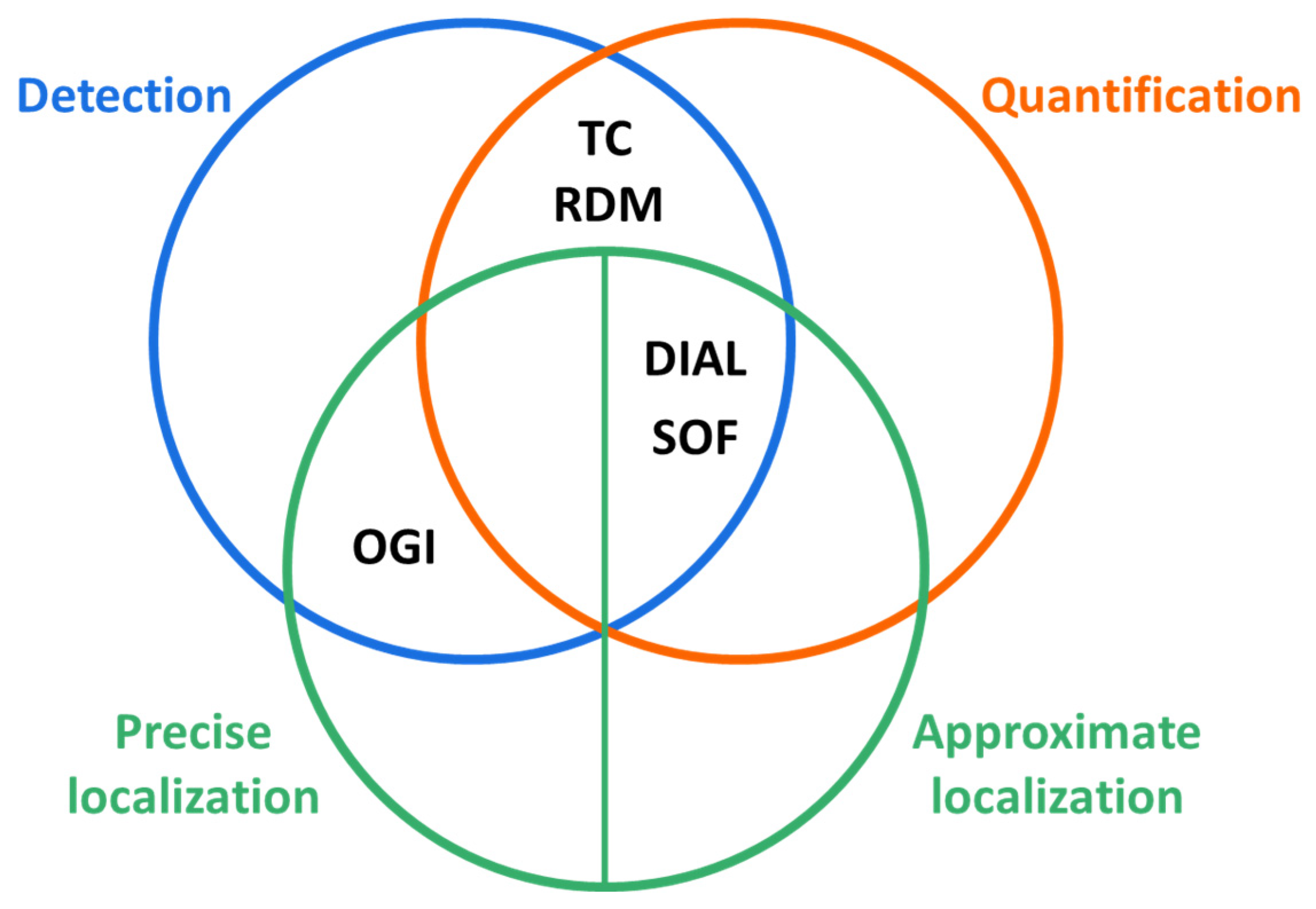
2.1. General Overview of the Standard
- Differential Infrared Absorption Lidar (DIAL)
- Solar Occultation Flux (SOF)
- Tracer Correlation (TC)
- Optical Gas Imaging (OGI)
- Reverse Dispersion Modelling (RDM)
2.2. Monitoring Program and Technique Selection
- The detection of each emission source
- Its localization
- The quantification of the emission rate
- Purpose and objective of the monitoring
- Type of monitoring required (identification and/or localization and/or quantification)
- Spatial resolution (function of the chosen technique and the area to be monitored)
- Localization of the emission source
- Quantification of the emission rate
- Duration of the monitoring (to consider both stationary sources and emissions due to malfunctions and/or emergencies)
- Chemical species to be monitored
3. Discussion About the Monitoring Techniques Described in the Standard
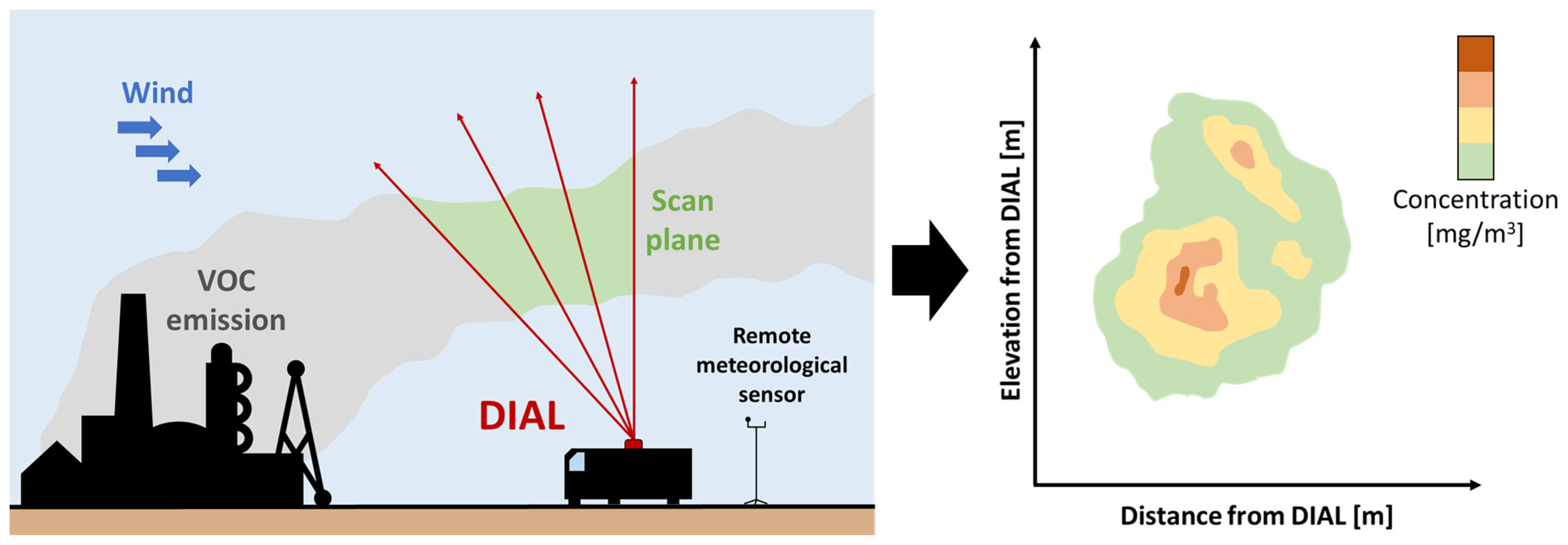
3.1. Differential Infrared Absorption Lidar (DIAL)
- The scanning system provides a two-dimensional concentration map in the air, allowing for the estimation of the plume’s shape and height. With a proper choice of scanning point, the technique can be used to visualize the specific area from which the plume extends, though it cannot pinpoint the exact emission source. For precise localization, a DIAL system may be complemented with an OGI thermographic inspection.
- The technique can quantify the mass flow emitted during the scan period of the perpendicular wind speed field to the scan plane, which can be estimated. The primary errors in quantifying flows arise from the description of the wind field.
- When positioned to perform a horizontal scan, the DIAL system can effectively identify significant emitters in the area (e.g., tank farms). However, the resolution (10 m) is not sufficient to identify individual significant point emitters.
- The DIAL system can quantify emissions from specific challenging sources. For example, it can determine emissions from flaring combustion if the flows and compositions sent to the flare are known, thus enabling the measurement of the flare’s efficiency and the implementation of emission factor estimates.
- The accuracy of emission rate measurements depends on weather conditions. Measurements cannot be conducted when visibility is significantly reduced due to fog or rain, or under very low wind conditions.
- To ideally obtain emitted mass flows, each concentration measurement point must be multiplied by the perpendicular wind speed component at the same spatial point. This is impracticable because the wind field cannot be measured at the exact concentration measurement point. Additionally, the emission plume near the source may be in the building downwash zone, causing the wind profile to vary with distance and differ significantly from open field conditions. This can lead to significant overestimation of the emission flow.
- Background concentrations upwind of the investigated source must be subtracted from downwind measurements. However, with only one DIAL system, it is not possible to simultaneously measure the upwind and downwind of the emission source. The DIAL setup involves large mobile containers (e.g., the NPL van is 12 m long), and moving and re-establishing these for upwind measurements takes considerable time (about an hour). During short-term monitoring campaigns, only one upstream scan might be feasible, making it impossible to determine if intermittent upstream sources influenced downwind measurements.
- Single-source measurements are typically performed over short periods, in fact, five to ten scans provide 1 to 2 h of measurement. Emissions in facilities like petrochemical plants and refineries often vary temporally. Thus, short-term DIAL measurements can only provide a “snapshot” of the emission flow from these sources. While DIAL data can help identify significant emitters, extrapolating to provide long-term estimates can lead to significant errors.
- Many hydrocarbon absorption spectra detected by DIAL overlap, and water vapor interference is certain. Operators often use the absorption frequency that gives strong signals for a typical hydrocarbon mixture in a refinery. The wavelength of a typical refinery hydrocarbon mixture spans from the visible to the mid-IR region, roughly between 0.5 and 2 μm [50]. This will cause systematic errors if the investigated pollutant has absorption characteristics significantly different from the standard hydrocarbon mixture (e.g., a mixture of propane and pentane when evaluating total hydrocarbons).
- Currently, only one company in the world (NPL) offers the DIAL system for commercial purposes.
- The system requires a team of no less than two highly prepared professionals. Typically, a measurement campaign at an industrial plant usually spans around 10 working days, with total costs > €10,000 per day.
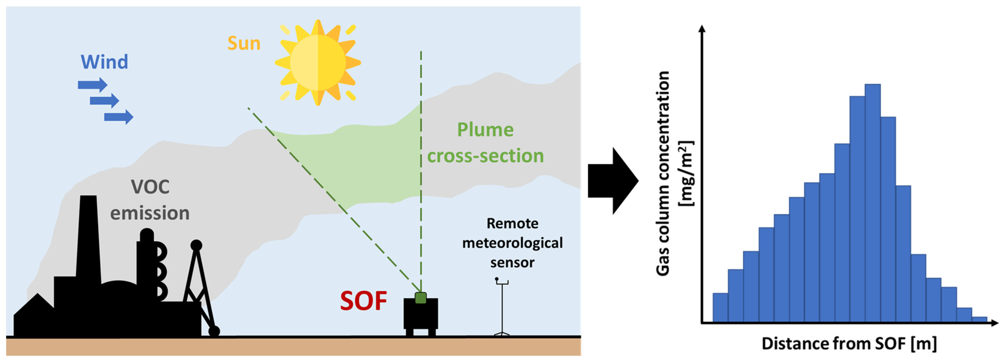
3.2. Solar Occultation Flux (SOF)
- Despite being a recent development, the technique has been used internationally in several projects and can be considered well established.
- The quantification of emitted mass flux can be carried out if a reasonable estimate of the wind field can be determined during the measurement period. As with DIAL, the main error in determining the flux is introduced by wind field data.
- The method is simpler than DIAL. The measurements are based on spectroscopic techniques, simultaneously enabling the identification and quantification of various species, including alkanes and alkenes. Aromatics, however, cannot be directly measured. Therefore, an overview of emissions from an industrial site can be mapped relatively quickly compared to the DIAL method, considering the ability of this technique to detect numerous species simultaneously, at the cost of obtaining a more limited amount of information.
- It is a costly but more affordable technique compared to using a DIAL system. A typical monitoring in an oil and gas plant may cost > €5000 per day, with a measurement duration of 8–10 days. However, the entire survey can take up to a month if the weather is not suitable for using SOF.
- When applied to near-field measurements, this technique can serve as an effective tool for identifying major emission sources, although uncertainties in emitted flux measurements for single equipment are higher compared to using it on entire plants. SOF can potentially be used to provide better quantification of significant emitters. However, the resolution is not sufficient to allow for the identification of individual emission points.
- Like DIAL, it allows the quantification of specific challenging sources. For example, it can determine emissions from flare combustion. If the flows and compositions sent there are known, it also allows measuring the efficiency of the flare itself and implementing the estimation of emission factors.
- The SOF technique uses the sun as a source of IR radiation. It can only be used during the day and only when sufficient sunlight is available for adequate measurement conditions. It is important to note that emissions from loading operations are typically higher during daytime working hours, with solar radiation further elevating certain VOC emissions, such as those from leaks in storage tanks.
- The SOF technique offers a measurement of the average concentration of a compound across the entire atmospheric column between the sun and the spectrometer. It cannot, therefore, provide concentration details along the length of the column to allow the identification of individual sources.
- Aromatic species cannot be directly measured with this technique. These compounds can be quantified using alternative methods to establish average concentration ratios relative to pollutants that are directly measured.
- To obtain emitted mass fluxes, it is necessary to multiply the concentration data by the wind speed component at the height of the smoke column. This cannot be achieved de facto since the height of the smoke column is actually unknown. This error can be limited when measurements are taken at a distance of a few hundred meters to several km, due to more homogenous wind fields away from the high surface roughness present in an industrial site. However, in cases where the plant under study is surrounded by other industrial structures, this distant measurement strategy may not be possible. Near-source measurements can result in an overestimation of the emission flux. Since the emission column near the source may be in the downwind depression zone of the structure itself (i.e., building downwash), the wind field profile along the scan line will vary with distance and will be significantly different from that measured in an area with flat terrain.
- Upstream emission data must be subtracted from those measured downstream of the investigated source. The SOF technique’s strategy involves driving the detection system around a plant while performing continuous measurements, both upstream and downstream. To reduce the uncertainty, several measurement circuits are necessary.
- SOF measurements are performed for relatively short periods and only during daylight hours. These measurements can only provide a short-term “snapshot” of emissions with temporal variations. Data obtained through SOF can help identify possible significant emitters, but extrapolation to provide long-term estimates can lead to significant errors.
- Only one company in the world commercially provides SOF measurements.
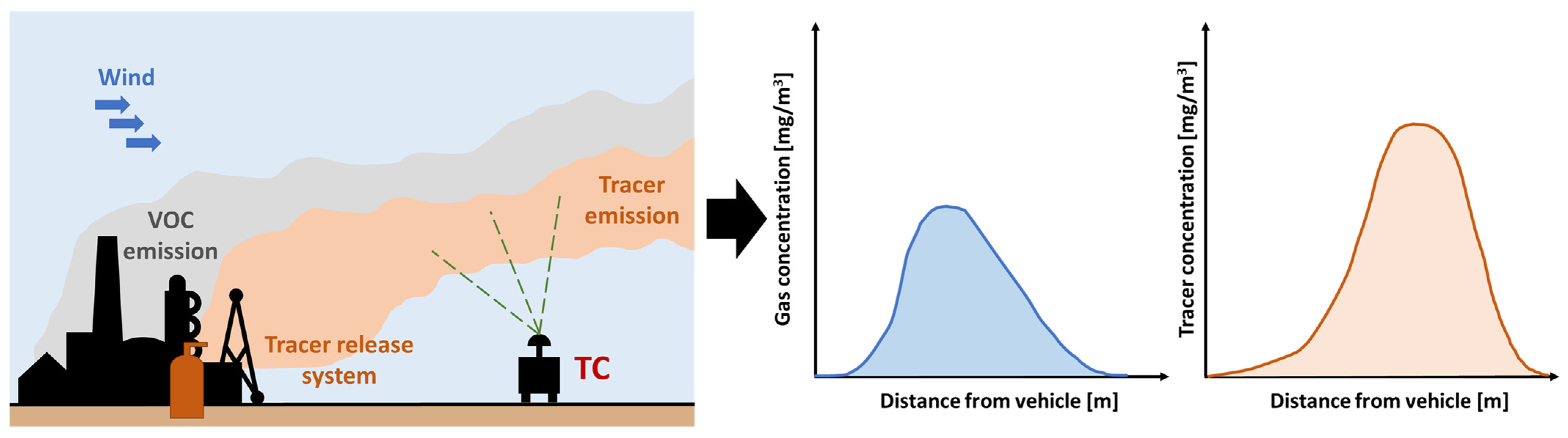
3.3. Tracer Correlation (TC)
- The detection system must be securely installed on a mobile platform, with a sampling port facing the ambient air.
- It must include sensors capable of measuring individual VOC species or the sum of different VOC species to be estimated (e.g., alkanes, alkenes, alcohols, or aromatics) and, simultaneously, one or more tracer gas species.
- It must measure the tracer gas with a detection limit below 10 μg/m3, and for the source gas, above 20 μg/m3, while the vehicle is in motion.
- It must be able to conduct sampling for approximately 10 min, with a data detection frequency below 10 s.
- It must display real-time data on tracer gas and VOC concentrations, as well as the position of the mobile system on the map.
- It must include a tracer gas release device capable of maintaining a mass flow rate between 0.1 kg/h and 10 kg/h.
- It is a well-established technique, particularly when the source is isolated and the aim is to measure or verify the mass flow rate emitted.
- With a known release from a particular source, there are no significant issues attributable to the upwind contributions with respect the emission source.
- Various tracers are available, sometimes identifiable in the emission itself given the composition of the plume.
- The technique is relatively low-cost, defined mainly by the placement of the controlled release system for the tracer rather than the instruments used to detect ground concentrations (Photoionization Detector, i.e., PID, or Flame Ionization Detector, i.e., FID).
- The potential source must be known for the placement of the controlled release system for the tracer.
- Significant calculation errors in the evaluation of the emission flow are possible, particularly due to the definition of the wind speed profile, especially near the source, where the flow is very complex.
- The tracer must be compatible with worker health and the site’s production. For accurate measurement, normal plant operation must be ensured.
- The technique is not suitable for chimneys or high-altitude sources, given the difficulty of evaluating ground concentrations of the tracer near the source.
- It is impossible to demonstrate the hypothesis underlying the method, i.e., the tracer follows the same advection and turbulent dispersion as the source gas.
3.4. Optical Gas Imaging (OGI)
- Recording emissions from variable sources for at least 20 s or as long as necessary to detect variability.
- Possibly acquire a video to capture the entire plume and surrounding context.
- Creating a visible image (non-IR) of the emission source.
- It requires high VOC concentrations and an appropriate background for plume visualization; it may not effectively detect very diluted emissions or sources subject to rapid dispersion.
- It cannot detect emissions from large equipment or plant sections due to plume dilution.
- Emission quantification is theoretically impossible with OGI, which only provides a qualitative assessment of potential emission sources.
- Experience shows that a team of two people using an OGI camera can typically inspect about 2000 equipment components per day. This performance is primarily influenced by the time needed to tag components identified as leaks for repair, as the camera operator must relay the location to the assistant. Conventional sniffing techniques, i.e., using PID/FID, are about four times slower (i.e., approximately 500 equipment components can be checked per day).
- All equipment components can be checked. This allows for the detection of large leaks in non-accessible positions, which would remain undetected in conventional sniffing monitoring.
- Current OGI cameras are the size and weight of household camcorders. This allows these instruments to be carried into process areas and tank roofs, which is not possible with more complex systems.
- Two or three days of training are needed to enable the use. Unlike sniffing, the camera does not necessitate instrument calibration, which consequently lowers the required skill level for the operation.
- The OGI technique is less effective than conventional sniffing methods in rain or fog. It also loses effectiveness in the presence of limited temperature differences with the surrounding environment.
- The price of commercially available camera systems varies from €40,000 to €100,000. In contrast, VOC detectors used in conventional sniffing surveys range from €5000 to €25,000, depending on their complexity. However, multiple detectors are often required to conduct a comprehensive site survey within a short timeframe.
- OGI cameras are generally not fully ATEX-rated, and work permits require the use of an explosion meter to check inspection areas. Conversely, detectors used in conventional sniffing surveys are rated for use in hazardous areas.
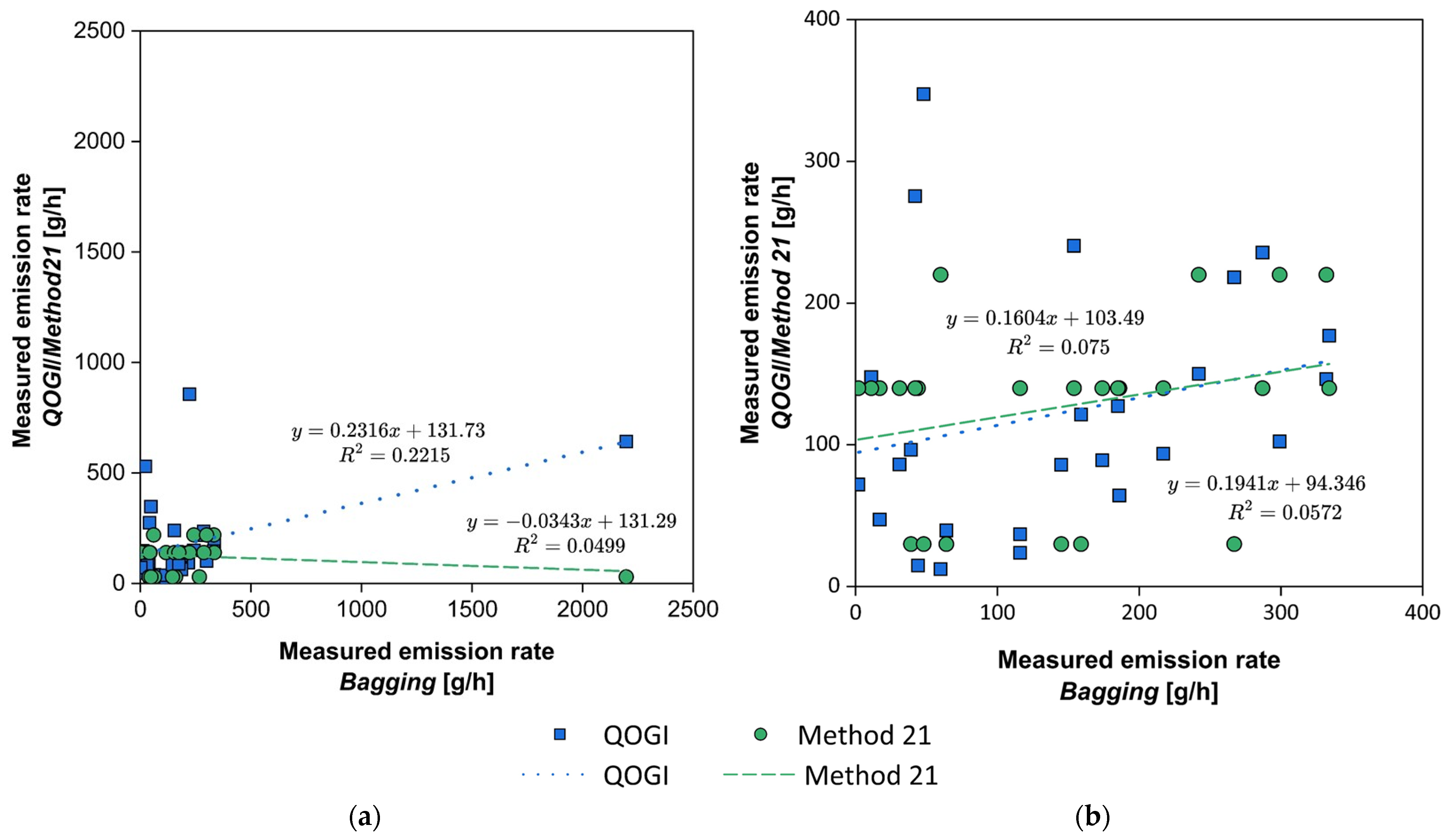
Quantitative Optical Gas Imaging (QOGI)
3.5. Reverse Dispersion Modelling (RDM)
- Avoid measuring concentration data too close to the emission source, considering a distance of at least 10 times the height of the emission source [82].
- The distance of the concentration detector from the source should be such that it captures a noticeable variation from the background concentration [82].
- Periods of high atmospheric stability may lead to a loss of accuracy in the emission estimates and should be therefore excluded [82].
- It is a well-established technique, already used and internationally regulated (EN 15445) for dust dispersion evaluation. Additionally, atmospheric dispersion models are widely used in evaluating the ground-level impacts of industrial emissions.
- It has relatively low costs compared to other techniques mentioned in this document, mainly attributable to ground concentration field detection using a traditional sniffing method (PID/FID).
- 3.
- The modeling is heavily influenced by the provided meteorological data, particularly wind direction and speed, and ground-level concentration measurements.
- 4.
- It is not possible to distinguish contributions from potential upwind sources in the observed area.
- 5.
- Correct model implementation requires source localization, using other detection and identification techniques.
- 6.
- In the presence of multiple sources or even multi-company sites, obtaining a single flow of data requires simultaneous data for each source. This is characterized by significant practical difficulties, both in locating each source and in measuring the various concentration values needed.
- 7.
- It is not suitable for evaluating high sources, due to difficulty in measuring ground concentrations near the sources.
4. Summary and Comparison of the Described Techniques
5. Review of Case Studies and Application of Techniques
5.1. Chronology of Comparative Studies Conducted
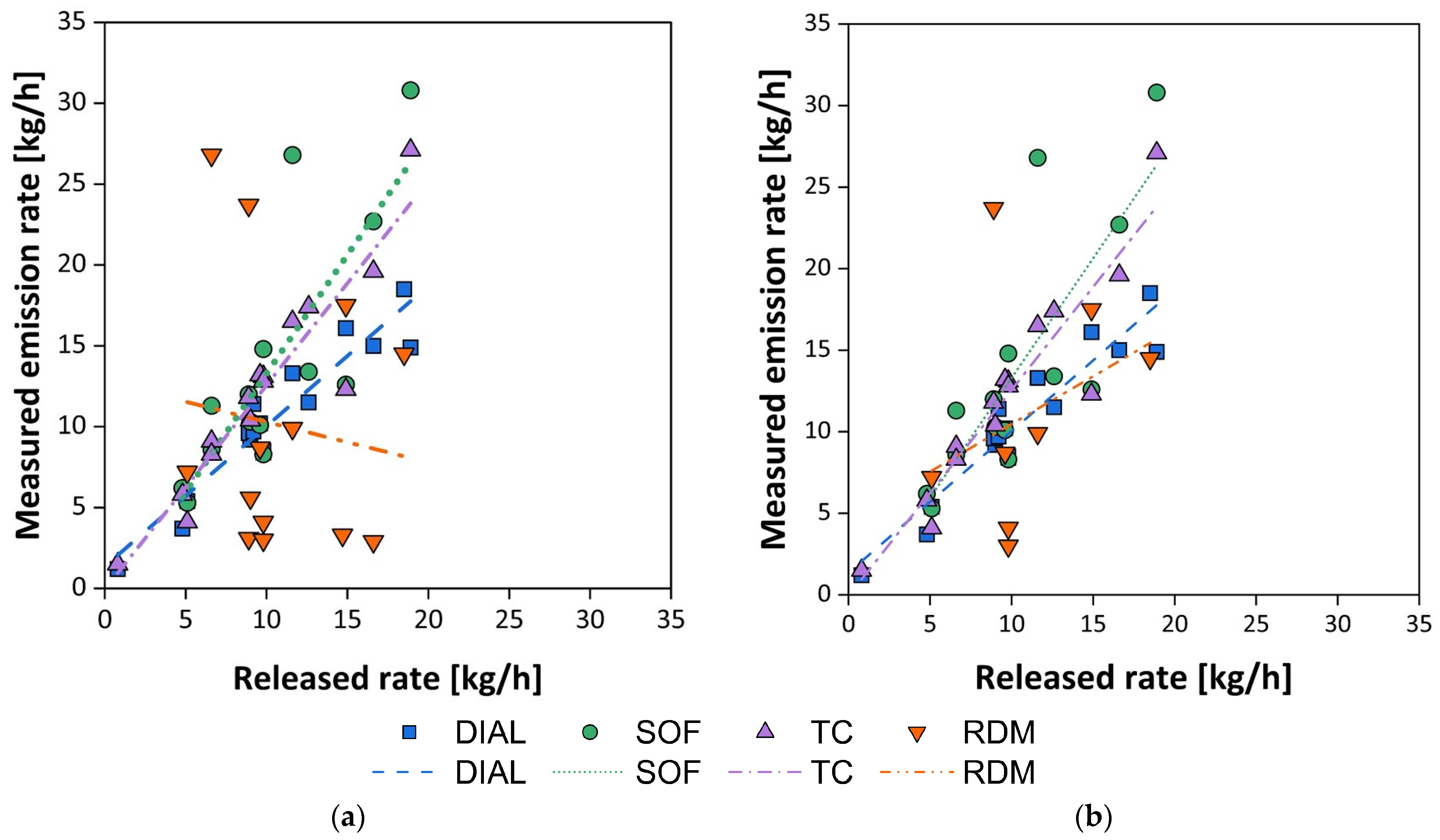
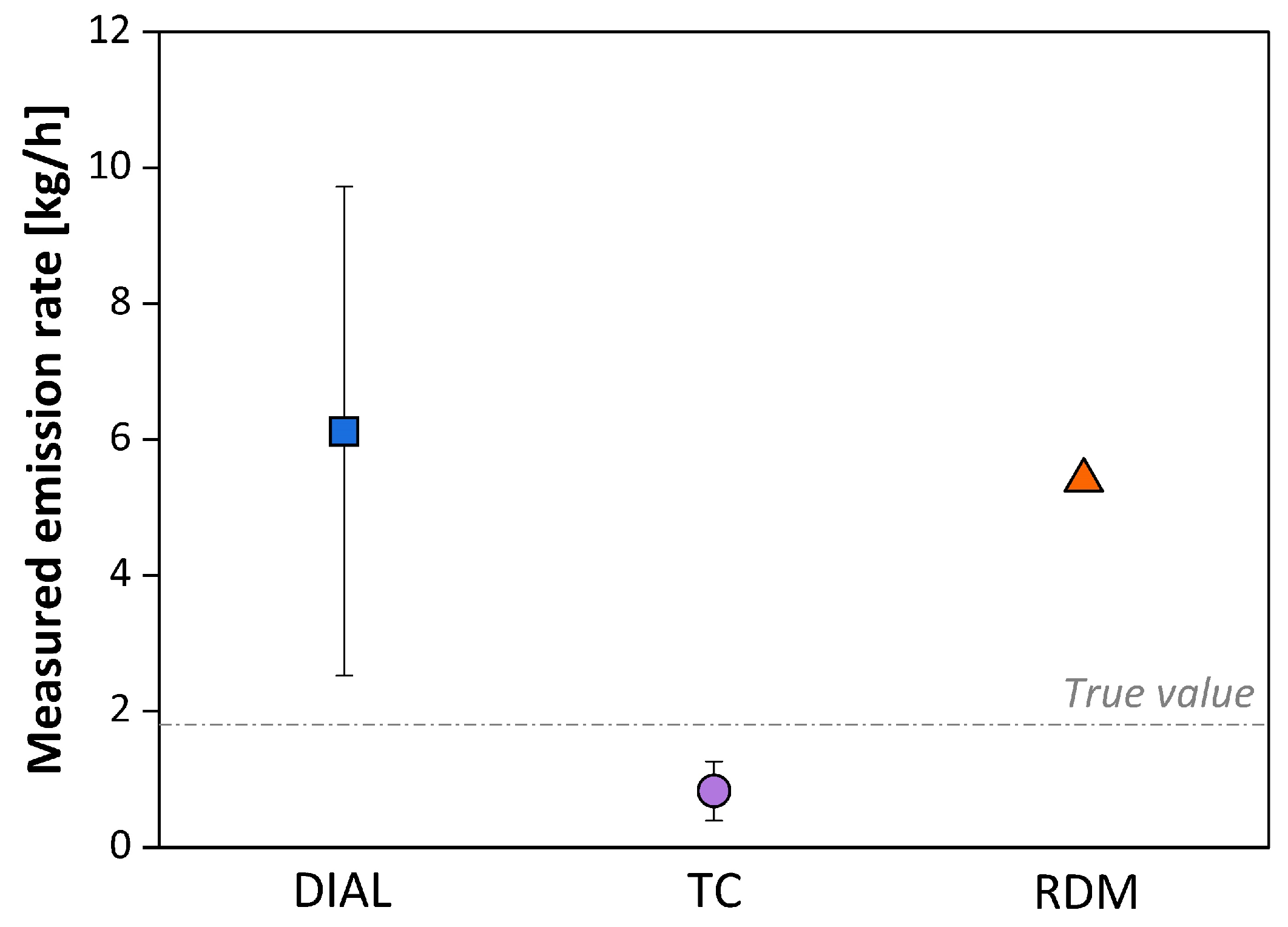
5.2. Comparison of Techniques with Controlled Release
- Bureau Veritas, as the operator of the OGI technique.
- NPL, as the operator of the DIAL technique.
- FluxSense and Chalmers University, as the operator of the SOF and TC techniques.
- Total, as the operator of the RDM technique.
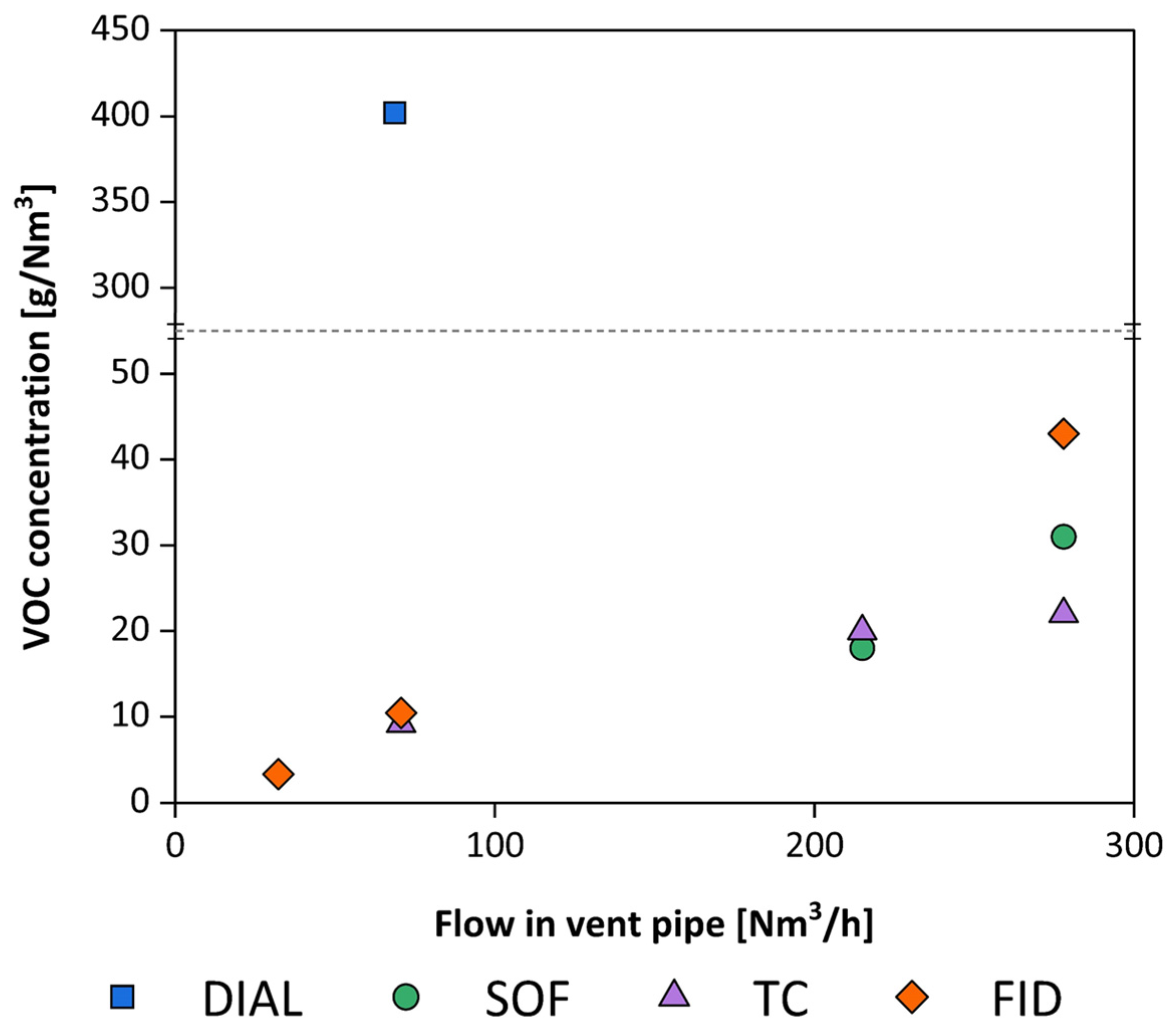
5.3. Comparison of Techniques in a Field Situation
5.4. Comparison of Techniques on Tank Measurements
6. Conclusions
Author Contributions
Funding
Conflicts of Interest
Abbreviations
| VOC | Volatile Organic Compound |
| DIAL | Differential Infrared Absorption Lidar |
| SOF | Solar Occultation Flux |
| TC | Tracer Correlation |
| OGI | Optical Gas Imaging |
| QOGI | Quantitative Optical Gas Imaging |
| RDM | Reverse Dispersion Modelling |
| BAT | Best Available Techniques |
| BREF | Best Available Techniques Reference |
| LDAR | Leak Detection and Repair |
| IR | Infrared Ray |
| UV | Ultra Violet |
| NPL | National Physical Laboratory |
| FTIR | Fourier Transform Infrared Ray |
| RPR | Release Precision Ratio |
| GWP | Global Warming Potential |
| PID | Photoionization Detector |
| FID | Flame Ionization Detector |
| ATEX | Atmosphères Explosives |
| API | America Petroleum Institute |
| SOCMI | Synthetic Organic Chemical Manufacturing Industry |
| EPA | Environmental Protection Agency |
| WG38 | Working Group 38 |
| VERI | Environnement Reasearch & Innovation |
| CRF | Controlled Release Facility |
| INERIS | Institut National de l’Environnement Industriel et des Risques |
| CFD | Computational Fluid Dynamic |
| SLAM | Safety Lagrangian Dispersion Model |
References
- Lin, Q.; Gao, Z.; Zhu, W.; Chen, J.; An, T. Underestimated contribution of fugitive emission to VOCs in pharmaceutical industry based on pollution characteristics, odorous activity and health risk assessment. J. Environ. Sci. 2022, 126, 722–733. [Google Scholar] [CrossRef] [PubMed]
- Cheng, L.; Wei, W.; Guo, A.; Zhang, C.; Sha, K.; Wang, R.; Wang, K.; Cheng, S. Health risk assessment of hazardous VOCs and its associations with exposure duration and protection measures for coking industry workers. J. Clean Prod. 2022, 379, 134919. [Google Scholar] [CrossRef]
- Duan, Z.; Lu, W.; Mustafa, M.F.; Du, J.; Wen, Y. Odorous gas emissions from sewage sludge composting windrows affected by the turning operation and associated health risks. Sci. Total Environ. 2022, 839, 155996. [Google Scholar] [CrossRef]
- Polvara, E.; Roveda, L.; Invernizzi, M.; Capelli, L.; Sironi, S. Estimation of Emission Factors for Hazardous Air Pollutants from Petroleum Refineries. Atmosphere 2021, 12, 1531. [Google Scholar] [CrossRef]
- Polvara, E.; Gallego, E.; Invernizzi, M.; Perales, J.F.; Sironi, S. Chemical characterization of odorous emissions: A comparative performance study of different sampling methods. Talanta 2022, 253, 124110. [Google Scholar] [CrossRef]
- Guerrero, T.N.; Le-Minh, N.; Fisher, R.M.; Prata, A.A.; Stuetz, R.M. Odour emissions from anaerobically co-digested biosolids: Identification of volatile organic and sulfur compounds. Sci. Total Environ. 2025, 959, 178192. [Google Scholar] [CrossRef]
- Vannevel, N.; Haerens, K.; Van Elst, T. Determination of the Sources Responsible for Odour Complaints in an Enclosed Working Space via the Use of Sensorial Analysis, GC-MS Analysis. Chem. Eng. Trans. 2024, 112, 67–72. [Google Scholar] [CrossRef]
- Parker, D.B. Reduction of odor and VOC emissions from a dairy lagoon. Appl. Eng. Agric. 2008, 24, 647–655. [Google Scholar] [CrossRef]
- Polvara, E.; Morosini, D.; Invernizzi, M.; Sironi, S. Analysis of Odorous VOCs using TD-GC-MS/FID/PFPD: Development and Applications to Real Samples. Chem. Eng. Trans. 2022, 95, 151–156. [Google Scholar] [CrossRef]
- European Commission. Best Available Techniques (BAT) Reference Document for the Refining of Mineral Oil and Gas. 2015. Available online: https://eippcb.jrc.ec.europa.eu/sites/default/files/2019-11/REF_BREF_2015.pdf (accessed on 15 December 2024).
- European Commission. JRC Reference Report on Monitoring of Emissions to Air and Water from IED Installations. 2018. Available online: https://eippcb.jrc.ec.europa.eu/sites/default/files/2019-12/ROM_2018_08_20.pdf (accessed on 15 December 2024).
- You, G.; Lu, S.; Jin, Z.; Ren, J.; Sun, R.; Li, J.; Hou, W.; Xie, S. Emission Factors and Source Profiles of Volatile Organic Compounds in the Petroleum Refining Industry through On-Site Measurement from Multiple Refineries. Environ. Sci. Technol. Lett. 2024, 11, 230–236. [Google Scholar] [CrossRef]
- Invernizzi, M.; Teramo, E.; Busini, V.; Sironi, S. A model for the evaluation of organic compounds emission from aerated liquid surfaces. Chemosphere 2020, 240, 124923. [Google Scholar] [CrossRef] [PubMed]
- Tagliaferri, F.; Invernizzi, M.; Sironi, S. Experimental evaluation on liquid area sources: Influence of wind velocity and temperature on the wind tunnel sampling of VOCs emissions from wastewater treatment plants. Chemosphere 2022, 312, 137337. [Google Scholar] [CrossRef]
- Sotoodeah, K. Storage Tanks Selection, Design, Testing, Inspection, and Maintenance; Elsevier: Amsterdam, The Netherlands, 2024. [Google Scholar] [CrossRef]
- Skaf, D.W.; Iervolino, T. Atmospheric Storage Tank Emission Estimates: Understanding the Calculation Basis and Effects of Uncertainty in Meteorological Inputs. J. Environ. Eng. 2019, 145, 04019089. [Google Scholar] [CrossRef]
- Yang, H.; Ren, B.; Huang, Y.; Zhang, Z.; Hu, W.; Liu, M.; Zhao, H.; Jiang, G.; Hao, Z. Volatile organic compounds (VOCs) emissions from internal floating-roof tank in oil depots in Beijing: Influencing factors and emission reduction strategies analysis. Sci. Total Environ. 2024, 916, 170222. [Google Scholar] [CrossRef]
- Invernizzi, M.; Sironi, S. Odour Emission Rate Estimation Methods for Hydrocarbon Storage Tanks. Chem. Eng. Trans. 2021, 85, 67–72. [Google Scholar] [CrossRef]
- Atasoy, E.; Döğeroğlu, T.; Kara, S. The estimation of NMVOC emissions from an urban-scale wastewater treatment plant. Water Res. 2004, 38, 3265–3274. [Google Scholar] [CrossRef] [PubMed]
- Fatone, F.; Di Fabio, S.; Bolzonella, D.; Cecchi, F. Fate of aromatic hydrocarbons in Italian municipal wastewater systems: An overview of wastewater treatment using conventional activated-sludge processes (CASP) and membrane bioreactors (MBRs). Water Res. 2010, 45, 93–104. [Google Scholar] [CrossRef] [PubMed]
- Zhang, Y.; Wei, C.; Yan, B. Emission characteristics and associated health risk assessment of volatile organic compounds from a typical coking wastewater treatment plant. Sci. Total Environ. 2019, 693, 133417. [Google Scholar] [CrossRef] [PubMed]
- Chambers, A.K.; Strosher, M.; Wootton, T.; Moncrieff, J.; McCready, P. Direct Measurement of Fugitive Emissions of Hydrocarbons from a Refinery. J. Air Waste Manag. Assoc. 2008, 58, 1047–1056. [Google Scholar] [CrossRef]
- Mo, Z.; Shao, M.; Lu, S.; Qu, H.; Zhou, M.; Sun, J.; Gou, B. Process-specific emission characteristics of volatile organic compounds (VOCs) from petrochemical facilities in the Yangtze River Delta, China. Sci. Total Environ. 2015, 533, 422–431. [Google Scholar] [CrossRef]
- Liu, Y.; Han, F.; Liu, W.; Cui, X.; Luan, X.; Cui, Z. Process-based volatile organic compound emission inventory establishment method for the petroleum refining industry. J. Clean. Prod. 2020, 263, 121609. [Google Scholar] [CrossRef]
- Guerrero, T.N.; Fisher, R.M.; Prata, A.A.; Stuetz, R. Sensory Assessment of Odour Emissions in Wastewater Treatment: Implications for Biosolids Management. Chem. Eng. Trans. 2024, 112, 73–78. [Google Scholar] [CrossRef]
- Tagliaferri, F.; Panzeri, F.; Invernizzi, M.; Manganelli, C.; Sironi, S. Characterization of diffuse odorous emissions from lignocellulosic biomass storage. J. Energy Inst. 2023, 112, 101440. [Google Scholar] [CrossRef]
- Hini, G.; Gao, K.; Zheng, Y.; Simayi, M.; Xie, S. Emission characteristics, OFPs, and Mitigation Perspectives of VOCs from Refining Industry in China’s Petrochemical Bases. Aerosol Air Qual. Res. 2023, 23, 220347. [Google Scholar] [CrossRef]
- Man, H.; Shao, X.; Cai, W.; Wang, K.; Cai, Z.; Xue, M.; Liu, H. Utilizing a optimized method for evaluating vapor recovery equipment control efficiency and estimating evaporative VOC emissions from urban oil depots via an extensive survey. J. Hazard. Mater. 2024, 479, 135710. [Google Scholar] [CrossRef]
- Invernizzi, M.; Roveda, L.; Polvara, E.; Sironi, S. Lights and Shadows of the Voc Emission Quantification. Chem. Eng. Trans. 2021, 85, 109–114. [Google Scholar] [CrossRef]
- Valastro, G. Guidance for Diffuse VOC Emission Determination Following EN 17628:2022. 2023, pp. 1–73. Available online: https://www.concawe.eu/publication/guidance-for-diffuse-voc-emission-determination-following-en-176282022/ (accessed on 15 December 2024).
- EN 17628:2022; Fugitive and Diffuse Emissions of Common Concern to Industry Sectors—Standard Method to Determine Diffuse Emissions of Volatile Organic Compounds into the Atmosphere. CEN: Brussels, Belgium, 2022. [CrossRef]
- European Commission. Commission Implementing Decision (EU) 06/12/2022 Establishing Best Available Techniques (BAT) Conclusions, Under Directive 2010/75/EU of the European Parliament and of the Council, for Common Waste Gas Management and Treatment Systems in the Chemical Sector. 2022. Available online: https://eur-lex.europa.eu/eli/dec_impl/2022/2427/oj/eng (accessed on 15 December 2024).
- European Commission. Commission Implementing Decision (EU) 2016/902 of 30 May 2016 Establishing Best Available Techniques (BAT) Conclusions, Under Directive 2010/75/EU of the European Parliament and of the Council, for Common Waste Water and Waste Gas Treatment/Management Systems in the Chemical Sector. 2016. Available online: https://eur-lex.europa.eu/eli/dec_impl/2016/902/oj/eng (accessed on 15 December 2024).
- Flesch, T.K.; Harper, L.A.; Coates, T.W.; Carlson, J. Estimation of gas emissions from a waste pond using micrometeorological approaches: Footprint sensitivities and complications. Atmos. Environ. X 2023, 19, 100219. [Google Scholar] [CrossRef]
- Lotesoriere, B.J.; Invernizzi, M.; Panzitta, A.; Uvezzi, G.; Sozzi, R.; Sironi, S.; Capelli, L. Micrometeorological Methods for the Indirect Estimation of Odorous Emissions. Crit. Rev. Anal. Chem. 2022, 53, 1531–1560. [Google Scholar] [CrossRef]
- Laubach, J.; Flesch, T.K.; Ammann, C.; Bai, M.; Gao, Z.; Merbold, L.; Campbell, D.I.; Goodrich, J.P.; Graham, S.L.; Hunt, J.E.; et al. Methane emissions from animal agriculture: Micrometeorological solutions for challenging measurement situations. Agric. For. Meteorol. 2024, 350, 109971. [Google Scholar] [CrossRef]
- European Commission. Directive 2010/75/EU of the European Parliament and of the Council of 24 November 2010 on Industrial Emissions (Integrated Pollution Prevention and Control). 2010. Available online: https://www.fao.org/faolex/results/details/en/c/LEX-FAOC109066/ (accessed on 15 December 2024).
- European Commission. Commission Implementing Decision of 9 October 2014 Establishing Best Available Techniques (BAT) Conclusions, under Directive 2010/75/EU of the European Parliament and of the Council on Industrial Emissions, for the Refining of Mineral Oil and Gas. Available online: https://eur-lex.europa.eu/eli/dec_impl/2014/738/oj/eng (accessed on 15 December 2024).
- M514 EN: Standardisation Mandate to CEN, CENELEC and ETSI Under Directive 2010/75/EU for a European Standard Method to Determine Fugitive and Diffuse Emissions of Volatile Organic Compounds (VOC) from Certain Industrial Sources to the Atmosphere. 2012. Available online: https://law.resource.org/pub/eu/mandates/m514.pdf (accessed on 15 December 2024).
- EN 15446:2008-04; Fugitive and Diffuse Emissions of Common Concern to Industry Sectors—Measurements of Fugitive Emission of Vapours Generating from Equipment and Piping Leaks. CEN: Brussels, Belgium, 2008. [CrossRef]
- McCorkle, B. Smart LDAR. In EPA Annual Natural Gas STAR Workshop; 2006. Available online: https://19january2021snapshot.epa.gov/sites/static/files/2017-06/documents/mccorkle_0.pdf (accessed on 15 December 2024).
- Robinson, R.; Gardiner, T.; Innocenti, F.; Woods, P.; Coleman, M. Infrared differential absorption Lidar (DIAL) measurements of hydrocarbon emissions. J. Environ. Monit. 2011, 13, 2213–2220. [Google Scholar] [CrossRef]
- Innocenti, F.; Gardiner, T.; Robinson, R. Uncertainty Assessment of Differential Absorption Lidar Measurements of Industrial Emissions Concentrations. Remote. Sens. 2022, 14, 4291. [Google Scholar] [CrossRef]
- HITRAN Database. Available online: https://hitran.org/ (accessed on 17 December 2024).
- NIST Standard Reference Database Number 69. 2023. Available online: https://doi.org/10.18434/T4D303 (accessed on 17 December 2024).
- NPL. Available online: https://www.npl.co.uk/products-services/environmental/absorption-lidar-dial (accessed on 17 December 2024).
- Rod, R. Review of the use of remote optical techniques for emission monitoring. In Proceedings of the EMPA: CEM 2007 8th International Conference in Emissions Monitoring, Zürich, Switzerland, 5–6 September 2007. [Google Scholar]
- Murray, E.R. Remote Measurement of Gases Using Differential-Absorption Lidar. Opt. Eng. 1978, 17, 170130. [Google Scholar] [CrossRef]
- Platt, U.; Perner, D.; Pätz, H.W. Simultaneous measurement of atmospheric CH2O, O3, and NO2 by differential optical absorption. J. Geophys. Res. Ocean. 1979, 84, 6329–6335. [Google Scholar] [CrossRef]
- Venkataramanan, L.; Fujisawa, G.; Mullins, O.C.; Vasques, R.R.; Valero, H.-P. Uncertainty Analysis of Visible and Near-Infrared Data of Hydrocarbons. Appl. Spectrosc. 2006, 60, 653–662. [Google Scholar] [CrossRef] [PubMed]
- Galle, B.; Mellqvist, J.; Arlander, D.W.; Fløisand, I.; Chipperfield, M.; Lee, A.M. Ground Based FTIR Measurements of Stratospheric Species from Harestua, Norway During SESAME and Comparison with Models. J. Atmos. Chem. 1999, 32, 147–164. [Google Scholar] [CrossRef]
- University of Texas Libraries. Available online: https://guides.lib.utexas.edu/az.php (accessed on 17 December 2024).
- Mellqvist, J. Application of Infrared and UV-Visible Remote Sensing Techniques for Studying the Stratosphere and for Estimating Antrophogenic Emissions. Ph.D. Thesis, Chalmers University of Technology, Goteborg, Sweden, 1999. [Google Scholar]
- Mellqvist, J.; Galle, B. Utveckling av ett IR Absorptionssystem Användande Solljus för Mätning av Diffusa Kolväteemissioner. 1999. Available online: https://research.chalmers.se/publication/540618/file/540618_Fulltext.pdf (accessed on 15 December 2024).
- FluxSense. Available online: https://www.fluxsense.com/technology/solar-occultation-flux-sof/ (accessed on 17 December 2024).
- Mellqvist, J.; Samuelsson, J.; Rivera, C.; Lefer, B.; Patel, M. Measurements of industrial emissions of VOCs, NH3, NO2 and SO2 in Texas using the Solar Occultation Flux method and mobile DOAS. Final. Rep. HARC Proj. H 2007, 53, 2–69. [Google Scholar]
- Bénassy, M.F.; Bilinska, K.; De Caluwé, G.; Ekstrom, L.; Leotoing, F.; Mares, I.; Roberts, P.; Smithers, B.; White, L.; Post, L. Optical methods for remote measurement of diffuse VOCs: Their role in the quantification of annual refinery emissions. In CONCAWE Reports; Concawe: Brussels, Belgium, 2008. [Google Scholar]
- Lamb, B.; Westberg, H.; Allwine, G. Isoprene emission fluxes determined by an atmospheric tracer technique. Atmos. Environ. 1986, 20, 1–8. [Google Scholar] [CrossRef]
- Howard, T.; Lamb, B.K.; Bamesberger, W.L.; Zimmerman, P.R. Measurement of VOC emission fluxes from waste treatment and disposal system using an atmospheric tracer flux. J. Air Waste Manag. Assoc. 1992, 42, 1336–1344. [Google Scholar] [CrossRef]
- Galle, B.; Samuelsson, J.; Svensson, B.H.; Börjesson, G. Measurements of Methane Emissions from Landfills Using a Time Correlation Tracer Method Based on FTIR Absorption Spectroscopy. Environ. Sci. Technol. 2000, 35, 21–25. [Google Scholar] [CrossRef]
- Delre, A.; Mønster, J.; Samuelsson, J.; Fredenslund, A.M.; Scheutz, C. Emission quantification using the tracer gas dispersion method: The influence of instrument, tracer gas species and source simulation. Sci. Total Environ. 2018, 634, 59–66. [Google Scholar] [CrossRef]
- Scheutz, C.; Kjeldsen, P. Guidelines for landfill gas emission monitoring using the tracer gas dispersion method. Waste Manag. 2019, 85, 351–360. [Google Scholar] [CrossRef]
- Czepiel, P.M.; Mosher, B.; Harriss, R.C.; Shorter, J.H.; McManus, J.B.; Kolb, C.E.; Allwine, E.; Lamb, B.K. Landfill methane emissions measured by enclosure and atmospheric tracer methods. J. Geophys. Res. Atmos. 1996, 101, 16711–16719. [Google Scholar] [CrossRef]
- Foster-Wittig, T.A.; Thoma, E.D.; Albertson, J.D. Estimation of point source fugitive emission rates from a single sensor time series: A conditionally-sampled Gaussian plume reconstruction. Atmos. Environ. 2015, 115, 101–109. [Google Scholar] [CrossRef]
- U.S. Environmental Protection Agency—Federal Register. Alternative Work Practice to Detect Leaks from Equipment. Available online: https://www.federalregister.gov/documents/2008/12/22/E8-30196/alternative-work-practice-to-detect-leaks-from-equipment (accessed on 17 December 2024).
- U.S. Environmental Protection Agency—Appendix K—Determination of Volatile Organic Compound and Greenhouse Gas Leaks Using Optical Gas Imaging. Available online: https://www.epa.gov/system/files/documents/2021-11/40-cfr-part-60-appendix-k-proposal_0.pdf (accessed on 17 December 2024).
- FLIR. Available online: https://www.flir.it/instruments/optical-gas-imaging/ (accessed on 17 December 2024).
- Panek, J.; Drayton, P.; Fashimpaur, D. Controlled laboratory sensitivity and performance evaluation of optical leak imaging infrared cameras for identifying alkane, alkene, and aromatic compounds. In Proceedings of the 99th Annual Conference and Exposition of the Air and Waste Management Association, New Orleans, LA, USA, 20–23 June 2006. [Google Scholar]
- Buttini, P. Infrared gas imaging and quantification camera for LDAR applications. In Proceedings of the AWMA 99th Annual Meeting, New Orleans, LA, USA, 20–23 June 2006. [Google Scholar]
- Benson, R.; Madding, R.; Lucier, R. Standoff passive optical leak detection of volatile organic compound using a cooled InSb based infrared imager. In Proceedings of the 99th Annual Conference and Exposition of the Air and Waste Management Association, New Orleans, LA, USA, 20–23 June 2006. [Google Scholar]
- Kangas, P.; Roberts, P.; Smithers, B.; Vaskinen, K.; Caico, C.; Tupper, P.; Negroni, J.; Gelpi, L.; Juery, C. Techniques for Detecting and Quantifying Fugitive Emissions—Results of Comparative Field Studies. In CONCAWE Reports; Concawe: Brussels, Belgium, 2015; Available online: https://www.concawe.eu/wp-content/uploads/rpt_15-6.pdf (accessed on 15 December 2024).
- Lev-On, M.; Epperson, D.; Siegell, J.; Ritter, K. Derivation of New Emission Factors for Quantification of Mass Emissions When Using Optical Gas Imaging for Detecting Leaks. J. Air Waste Manag. Assoc. 2007, 57, 1061–1070. [Google Scholar] [CrossRef] [PubMed]
- Cangialosi, F.; Milella, L.; Fornaro, A. Assessing the Significance of Fugitive Emissions from a Landfill Biogas Collecting System using a Quantitative Optical Gas Imaging (QOGI) Method: A Case Study. Chem. Eng. Trans. 2024, 112, 19–24. [Google Scholar] [CrossRef]
- Bergau, M.; Scherer, B.; Knoll, L.; Wöllenstein, J. Active gas camera mass flow quantification (qOGI): Application in a biogas plant and comparison to state-of-the-art gas cams. Rev. Sci. Instrum. 2024, 95, 063702. [Google Scholar] [CrossRef]
- Yousheng, Z. Rediscovering infrared cameras. In Proceedings of the 4C HSE Conference, Austin, TX, USA, 22–25 February 2016. [Google Scholar]
- Hoven, L.; Kangas, P.; Megaritis, T. Results of a Comparative Pilot Field Test Study of a First Generation Quantitative Optical Gas Imaging (QOGI) System. In CONCAWE Reports; Concawe: Brussels, Belgium, 2020; Available online: https://www.concawe.eu/publication/results-of-a-comparative-pilot-field-test-study-of-a-first-generation-quantitative-optical-gas-imaging-qogi-system/ (accessed on 15 December 2024).
- U.S. Environmental Protection Agency, EPA-453/R-95-017, Protocol for Equipment Leak Emission Estimates. 1995. Available online: https://www.epa.gov/sites/default/files/2020-09/documents/protocol_for_equipment_leak_emission_estimates.pdf (accessed on 15 December 2024).
- Ilonze, C.; Wang, J.; Ravikumar, A.P.; Zimmerle, D. Methane Quantification Performance of the Quantitative Optical Gas Imaging (QOGI) System Using Single-Blind Controlled Release Assessment. Sensors 2024, 24, 4044. [Google Scholar] [CrossRef]
- Flesch, T.K.; Wilson, J.D.; Yee, E. Backward-Time Lagrangian Stochastic Dispersion Models and Their Application to Estimate Gaseous Emissions. J. Appl. Meteorol. 1995, 34, 1320–1332. [Google Scholar] [CrossRef]
- EN 15445:2008-04; Fugitive and Diffuse Emissions of Common Concern to Industry Sectors—Qualification of Fugitive Dust Sources by Reverse Dispersion Modelling. CEN: Brussels, Belgium, 2008. [CrossRef]
- Flesch, T.K.; McGinn, S.M.; Chen, D.; Wilson, J.D.; Desjardins, R.L. Data filtering for inverse dispersion emission calculations. Agric. For. Meteorol. 2014, 198–199, 1–6. [Google Scholar] [CrossRef]
- Flesch, T.K.; Wilson, J.D.; Harper, L.A.; Crenna, B.; Sharpe, R.R. Deducing Ground-to-Air Emissions from Observed Trace Gas Concentrations: A Field Trial. J. Appl. Meteorol. 2004, 43, 487–502. [Google Scholar] [CrossRef]
- Hu, N.; Flesch, T.K.; Wilson, J.D.; Baron, V.S.; Basarab, J.A. Refining an inverse dispersion method to quantify gas sources on rolling terrain. Agric. For. Meteorol. 2016, 225, 1–7. [Google Scholar] [CrossRef]
- Ro, K.S.; Johnson, M.H.; Stone, K.C.; Hunt, G.; Flesch, T.; Todd, R.W. Measuring gas emissions from animal waste lagoons with an inverse-dispersion technique. Atmos. Environ. 2012, 66, 101–106. [Google Scholar] [CrossRef]
- Gardiner, T.; Helmore, J.; Innocenti, F.; Robinson, R. Field Validation of Remote Sensing Methane Emission Measurements. Remote. Sens. 2017, 9, 956. [Google Scholar] [CrossRef]
- Innocenti, F.; Robinson, R.; Gardiner, T.; Finlayson, A.; Connor, A. Differential Absorption Lidar (DIAL) Measurements of Landfill Methane Emissions. Remote. Sens. 2017, 9, 953. [Google Scholar] [CrossRef]
- Bourn, M.; Robinson, R.; Innocenti, F.; Scheutz, C. Regulating landfills using measured methane emissions: An English perspective. Waste Manag. 2018, 87, 860–869. [Google Scholar] [CrossRef] [PubMed]
- Johansson, J.K.E.; Mellqvist, J.; Samuelsson, J.; Offerle, B.; Lefer, B.; Rappenglück, B.; Flynn, J.; Yarwood, G. Emission measurements of alkenes, alkanes, SO2, and NO2 from stationary sources in Southeast Texas over a 5 year period using SOF and mobile DOAS. J. Geophys. Res. Atmos. 2014, 119, 1973–1991. [Google Scholar] [CrossRef]
- Johansson, J.K.E.; Mellqvist, J.; Samuelsson, J.; Offerle, B.; Moldanova, J.; Rappenglück, B.; Lefer, B.; Flynn, J. Quantitative measurements and modeling of industrial formaldehyde emissions in the Greater Houston area during campaigns in 2009 and 2011. J. Geophys. Res. Atmos. 2014, 119, 4303–4322. [Google Scholar] [CrossRef]
- Mellqvist, J.; Vechi, N.T.; Scheutz, C.; Durif, M.; Gautier, F.; Johansson, J.; Samuelsson, J.; Offerle, B.; Brohede, S. An uncertainty methodology for solar occultation flux measurements: Ammonia emissions from livestock production. Atmos. Meas. Tech. 2024, 17, 2465–2479. [Google Scholar] [CrossRef]
- Mellqvist, J.; Samuelsson, J.; Johansson, J.; Rivera, C.; Lefer, B.; Alvarez, S.; Jolly, J. Measurements of industrial emissions of alkenes in Texas using the solar occultation flux method. J. Geophys. Res. Atmos. 2010, 115, 1–13. [Google Scholar] [CrossRef]
- Börjesson, G.; Samuelsson, J.; Chanton, J.; Adolfsson, R.; Galle, B.; Svensson, B.H. A national landfill methane budget for Sweden based on field measurements, and an evaluation of IPCC models. Tellus B Chem. Phys. Meteorol. 2009, 61, 424. [Google Scholar] [CrossRef]
- Roscioli, J.R.; Yacovitch, T.I.; Floerchinger, C.; Mitchell, A.L.; Tkacik, D.S.; Subramanian, R.; Martinez, D.M.; Vaughn, T.L.; Williams, L.; Zimmerle, D.; et al. Measurements of methane emissions from natural gas gathering facilities and processing plants: Measurement methods. Atmos. Meas. Tech. 2015, 8, 2017–2035. [Google Scholar] [CrossRef]
- Mønster, J.; Samuelsson, J.; Kjeldsen, P.; Scheutz, C. Quantification of methane emissions from 15 Danish landfills using the mobile tracer dispersion method. Waste Manag. 2015, 35, 177–186. [Google Scholar] [CrossRef] [PubMed]
- Mønster, J.G.; Samuelsson, J.; Kjeldsen, P.; Rella, C.W.; Scheutz, C. Quantifying methane emission from fugitive sources by combining tracer release and downwind measurements—A sensitivity analysis based on multiple field surveys. Waste Manag. 2014, 34, 1416–1428. [Google Scholar] [CrossRef]
- Henne, S.; Brunner, D.; Oney, B.; Leuenberger, M.; Eugster, W.; Bamberger, I.; Meinhardt, F.; Steinbacher, M.; Emmenegger, L. Validation of the Swiss methane emission inventory by atmospheric observations and inverse modelling. Atmos. Meas. Tech. 2016, 16, 3683–3710. [Google Scholar] [CrossRef]
- Cui, Y.Y.; Brioude, J.; McKeen, S.A.; Angevine, W.M.; Kim, S.; Frost, G.J.; Ahmadov, R.; Peischl, J.; Bousserez, N.; Liu, Z.; et al. Top-down estimate of methane emissions in California using a mesoscale inverse modeling technique: The South Coast Air Basin. J. Geophys. Res. Atmos. 2015, 120, 6698–6711. [Google Scholar] [CrossRef]
- Seaton, M.; Leslie, I.; Stidworthy, A.; Jones, R.; Dicks, J.; Clarke, D.; Popoola, O.A.; Carruthers, D. Urban emission inventory optimisation using sensor data, an urban air quality model and inversion techniques. Int. J. Environ. Pollut. 2019, 66, 252. [Google Scholar] [CrossRef]
- Ravikumar, A.; Wang, J.; Brandt, A.R. Are Optical Gas Imaging Technologies Effective For Methane Leak Detection? Environ. Sci. Technol. 2016, 51, 718–724. [Google Scholar] [CrossRef]
- Cangialosi, F.; Bruno, E.; Fornaro, A. Integrating Citizen Science and Machine Learning Algorithms for the Recognition of Odour Classes nearby a Wastewater Treatment Plant. Chem. Eng. Trans. 2022, 95, 25–30. [Google Scholar] [CrossRef]
- Zhang, R.; Wang, H.; Tan, Y.; Zhang, M.; Zhang, X.; Wang, K.; Ji, W.; Sun, L.; Yu, X.; Zhao, J.; et al. Using a machine learning approach to predict the emission characteristics of VOCs from furniture. Build. Environ. 2021, 196, 107786. [Google Scholar] [CrossRef]
- Capman, N.S.S.; Zhen, X.V.; Nelson, J.T.; Chaganti, V.R.S.K.; Finc, R.C.; Lyden, M.J.; Williams, T.L.; Freking, M.; Sherwood, G.J.; Bühlmann, P.; et al. Machine Learning-Based Rapid Detection of Volatile Organic Compounds in a Graphene Electronic Nose. ACS Nano 2022, 16, 19567–19583. [Google Scholar] [CrossRef]
- Marco, S. Machine Learning and Artificial Intelligence. In Volatile Biomarkers for Human Health; The Royal Society of Chemistry: London, UK, 2022; pp. 454–471. [Google Scholar] [CrossRef]
- Smithers, B.; McKay, J.; Van Ophem, G.; Van Parijs, K.; White, L. VOC Emissions from External Floating Roof Tanks: Comparison of Remote Measurements by Laser with Calculation Methods; CONCAWE Reports: Helsinki, Finland, 1995; pp. 1–25. [Google Scholar]
- CEN/TC, Determination of Diffuse VOC Emissions. 2018. Available online: https://standards.iteh.ai/catalog/tc/cen/bac001c1-2de7-4a0e-aa44-9e6e8ead3514/cen-tc-264-wg-38 (accessed on 15 December 2024).
- Bai, M.; Velazco, J.I.; Coates, T.W.; Phillips, F.A.; Flesch, T.K.; Hill, J.; Mayer, D.G.; Tomkins, N.W.; Hegarty, R.S.; Chen, D. Beef cattle methane emissions measured with tracer-ratio and inverse dispersion modelling techniques. Atmos. Meas. Tech. 2021, 14, 3469–3479. [Google Scholar] [CrossRef]
- Babilotte, A.; Lagier, T.; Fiani, E.; Taramini, V. Fugitive Methane Emissions from Landfills: Field Comparison of Five Methods on a French Landfill. J. Environ. Eng. 2010, 136, 777–784. [Google Scholar] [CrossRef]
- Hrad, M.; Huber-Humer, M.; Reinelt, T.; Spangl, B.; Flandorfer, C.; Innocenti, F.; Yngvesson, J.; Fredenslund, A.; Scheutz, C. Determination of methane emissions from biogas plants, using different quantification methods. Agric. For. Meteorol. 2022, 326, 109179. [Google Scholar] [CrossRef]
- Thomson, D.J.; Manning, A.J. Along-wind dispersion in light wind conditions. Bound. Layer Meteorol. 2001, 98, 341–358. [Google Scholar] [CrossRef]
- Jeong, H.; Park, M.; Hwang, W.; Kim, E.; Han, M. The effect of calm conditions and wind intervals in low wind speed on atmospheric dispersion factors. Ann. Nucl. Energy 2013, 55, 230–237. [Google Scholar] [CrossRef]
- Tian, S.; Riddick, S.N.; Cho, Y.; Bell, C.S.; Zimmerle, D.J.; Smits, K.M. Investigating detection probability of mobile survey solutions for natural gas pipeline leaks under different atmospheric conditions. Environ. Pollut. 2022, 312, 120027. [Google Scholar] [CrossRef]
- Jones, F.M.; Phillips, F.A.; Naylor, T.; Mercer, N.B. Methane emissions from grazing Angus beef cows selected for divergent residual feed intake. Anim. Feed. Sci. Technol. 2011, 166–167, 302–307. [Google Scholar] [CrossRef]
- Griffith, D.W.T.; Bryant, G.R.; Hsu, D.; Reisinger, A.R. Methane Emissions from Free-Ranging Cattle: Comparison of Tracer and Integrated Horizontal Flux Techniques. J. Environ. Qual. 2008, 37, 582–591. [Google Scholar] [CrossRef]
- Flesch, T.K.; Vergé, X.C.; Desjardins, R.L.; Worth, D. Methane emissions from a swine manure tank in western Canada. Can. J. Anim. Sci. 2013, 93, 159–169. [Google Scholar] [CrossRef]
- American Petroleum Institute (API). Manual of Petroleum Measurement Standards. Chapter19: Evaporative Loss Measurements, Section 2: Evaporative Loss from Floating-Roof Tanks. 2005. Available online: https://standards.globalspec.com/std/210618/api-mpms-19-2 (accessed on 15 December 2024).
- American Petroleum Institute (API). Manual of Petroleum Measurement Standards. Chapter 19: Evaporative Loss Measurements, Section 1: Evaporative Loss from Fixed-Roof Tanks. 2003. Available online: https://standards.globalspec.com/std/10162292/api-mpms-19-1 (accessed on 15 December 2024).
- U.S. Environmental Protection Agency. Liquid Storage Tanks. 2024. Available online: https://www.epa.gov/natural-gas-star-program/storage-tanks (accessed on 15 December 2024).


| Parameter | DIAL | SOF | TC | RDM | OGI | QOGI |
|---|---|---|---|---|---|---|
| Measurement scale | 100 m–1 km (max resolution = 3 m) | 10 m–10 km (max resolution = 10 m) | 10 m–2 km (max resolution = 10 m) | Theoretically no limitation (in accordance with the model used) | <1 m | <1 m |
| Type of sources | Main plant equipments, plant section | Main plant equipments, plant section, entire industrial site | Main plant equipments | Main equipments, plant section | Components (pumps, valves, flanges, seals, …) | Components (pumps, valves, flanges, seals, …) |
| Role | Detection, localization, quantification | Detection, localization, quantification | Detection, quantification | Detection, quantification | Detection, localization | Detection, localization, quantification |
| Output | 2D concentration map in ppm, emissive mass flux in kg/h | Geolocated concentration columns in mg/m2, emissive mass flux in kg/h | Geolocated concentrations in μg/m3, emissive mass flux in kg/h | Concentration in mg/m3, emissive mass flux in kg/h | Plume visualization | Concentration in ppm∙m, Emissive mass flux in g/h |
| Measured compounds | Benzene, toluene, hydrocarbons C3+ (max two compounds at a time) | Alkanes (C2–C20), alcohols (C1–C8), alkenes (C2–C4), amines, aldehydes, dienes | Sensor selected based on the tracer (e.g., C2H2 or N2O) | No limitation (traditional PID/FID detection tools) | No complete list of detectable compounds is currently available (e.g., methane, benzene < 50 ppm∙m; ethylene, phenol < 150 ppm∙m) | No complete list of detectable compounds is currently available (e.g., methane, benzene < 50 ppm∙m; ethylene, phenol < 150 ppm∙m) |
| Measurement time | ~15 min per single scan (at least four scans required for a single measurement) | 1–2 s per single column (about 20 m base) | 1–5 min for point sources, 10 ÷ 20 min for areal sources | 30–60 min | About 1000 components per day per operator | About 1000 components per day per operator |
| Detection limits | 30 ppm in IR, 10 ppb in UV | 1–5 mg/m2 for concentrations, 1 kg/h for mass flux | 10 μg/m3 for concentrations, 0.1 kg/h for emissive flux | Function of the configuration of the emission source | 0.8 g/h for methane | 0.8 g/h for methane, 3.8 g/h for toluene, 0.7 g/h for ethanol |
| Measurement uncertainty | 5–25% | 21–37% | 20–40% | Largely dependent on meteorological conditions | No quantification | Not yet determined |
| Indicative costs of monitoring | 100,000–200,000 € | 50,000–150,000 € | 20,000–70,000 € | 30,000–100,000 € | 10,000–50,000 € | 25,000–60,000 € |
| References | [42,43,85,86,87] | [56,88,89,90,91] | [60,92,93,94,95] | [82,84,96,97,98] | [68,69,70,71,99] | [67,72,73,74,75] |
| Date | Location | Organizing Body | Techniques Involved | Reference |
|---|---|---|---|---|
| January 1995 | Not specified | CONCAWE | API algorithms, DIAL | [104] |
| Autumn 2000 | Sweden | CONCAWE | API algorithms, DIAL | [57] |
| June/July 2005 | Sweden | CONCAWE | SOF, TC, FID | [57] |
| June 2007 | Sweden | CONCAWE | API algorithms, OGI, TC | [57] |
| October 2007 | France | Veolia Environnement Reasearch & Innovation (VERI) | TC, DIAL, RDM | [105] |
| February 2013 | Australia | Australian Agency for International Development National Institute for Agricultural Research | TC, RDM | [106] |
| September 2016 | France | Working Group 38 | DIAL, SOF, TC, RDM | [107] |
| October 2016 May 2017 | Austria | ERA-NET Bioenergy | DIAL, TC, RDM | [108] |
| June 2017 | Netherlands | Working Group 38 | DIAL, SOF, TC, RDM | [107] |
| DIAL | SOF | TC | RDM | RDM, U > 2 m/s | |
|---|---|---|---|---|---|
| Slope (m) | 0.868 | 1.468 | 1.263 | −0.250 | 0.585 |
| Intercept (q) | 1.363 | −1.379 | −0.056 | 12.796 | 4.627 |
| R2 | 0.8965 | 0.6527 | 0.8782 | 0.0147 | 0.1138 |
| TC | DIAL | RDM | |
|---|---|---|---|
| Campaign duration (days) | 1.5 | 1.5 | 1.5 |
| Data analysis (hours) | 40 | 50 | 100 |
| Instrumentation cost (k€) | 100 | 1500 | 70 |
| Required personnel | 2 | 3 | 2 |
| Daily monitoring capacity (hectares/day) | >20 | 10 ÷ 15 | >20 |
| Tank | Tank Type | Content | Leaks Identified with OGI Camera | Emissions Estimated with API Algorithms [t/y] | Emissions Measured with TC Method [t/y] |
|---|---|---|---|---|---|
| T-105 | EFRT 1 | Crude oil | 1 | 3 | 4 |
| T-107 | EFRT 1 | Crude oil | 4 | 4 | 35 |
| T-108 | EFRT 1 | Crude oil | 22 | 4 | 120 |
| T-304 | IFRT 2 | Reforming gasoline | 0 | 0.2 | 0 |
| T-325 | FRT 3 | Fuel oil | 0 | 1 | 0 |
Disclaimer/Publisher’s Note: The statements, opinions and data contained in all publications are solely those of the individual author(s) and contributor(s) and not of MDPI and/or the editor(s). MDPI and/or the editor(s) disclaim responsibility for any injury to people or property resulting from any ideas, methods, instructions or products referred to in the content. |
© 2025 by the authors. Licensee MDPI, Basel, Switzerland. This article is an open access article distributed under the terms and conditions of the Creative Commons Attribution (CC BY) license (https://creativecommons.org/licenses/by/4.0/).
Share and Cite
Carrera, L.; Sironi, S.; Invernizzi, M. Toward Effective Monitoring of Diffuse VOC Emissions: A Critical Discussion and Review of the Applications of EN 17628:2022. Sensors 2025, 25, 1561. https://doi.org/10.3390/s25051561
Carrera L, Sironi S, Invernizzi M. Toward Effective Monitoring of Diffuse VOC Emissions: A Critical Discussion and Review of the Applications of EN 17628:2022. Sensors. 2025; 25(5):1561. https://doi.org/10.3390/s25051561
Chicago/Turabian StyleCarrera, Luca, Selena Sironi, and Marzio Invernizzi. 2025. "Toward Effective Monitoring of Diffuse VOC Emissions: A Critical Discussion and Review of the Applications of EN 17628:2022" Sensors 25, no. 5: 1561. https://doi.org/10.3390/s25051561
APA StyleCarrera, L., Sironi, S., & Invernizzi, M. (2025). Toward Effective Monitoring of Diffuse VOC Emissions: A Critical Discussion and Review of the Applications of EN 17628:2022. Sensors, 25(5), 1561. https://doi.org/10.3390/s25051561