
Measuring the Level of Aflatoxin Infection in Pistachio Nuts by Applying Machine Learning Techniques to Hyperspectral Images

 ,
,  ,
,  , and
, and
Abstract
1. Introduction
- Analyses and identifies the important wavelengths for effective detection of aflatoxins within pistachio nuts. The key wavelengths were identified as 399.98 nm, 584.64 nm, 704.64 nm, 866.21 nm, and 1002.23 nm.
- Rigorously evaluates multiple classifiers using only important wavelengths, such as 866.21 nm, to determine aflatoxin levels, demonstrating the effectiveness of ResNet with a 96.67% accuracy at wavelength 866.21 nm.
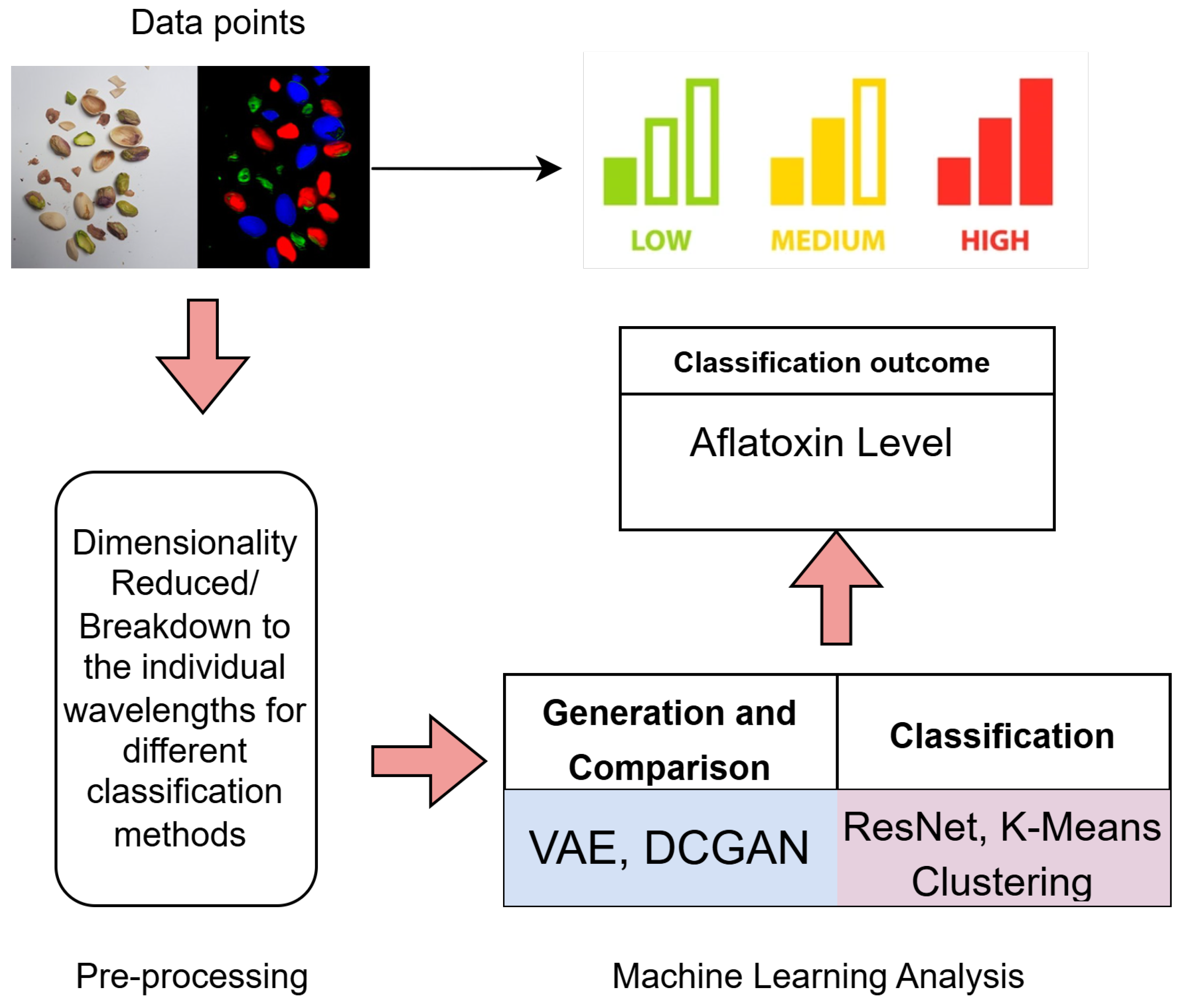
- Applies the unsupervised learning approach Dimensionality Reduction combined with K-Means Clustering to the entire hyperspectral image dataset to classify the images, thereby improving the computational time complexity of the K-Means algorithm through dimensionality reduction by at least 34,151.04 times.
2. Background
2.1. Pistachio Consumption and Industry
2.2. Aflatoxin Detection Within the Pistachio Industry
2.2.1. The Importance of Aflatoxin Detection Within the Pistachio Industry
2.2.2. Thin-Layer Chromatography
2.2.3. High-Performance Liquid Chromatography
2.2.4. Laser-Induced Fluorescence Spectroscopy
2.2.5. Summary
2.3. Hyperspectral Imaging
2.3.1. What Is Hyperspectral Imaging?
2.3.2. Hyperspectral Imaging in the Nut Industry
2.3.3. Analysis of Hyperspectral Images of Pistachios
2.3.4. Summary and Insights
3. Materials and Methods
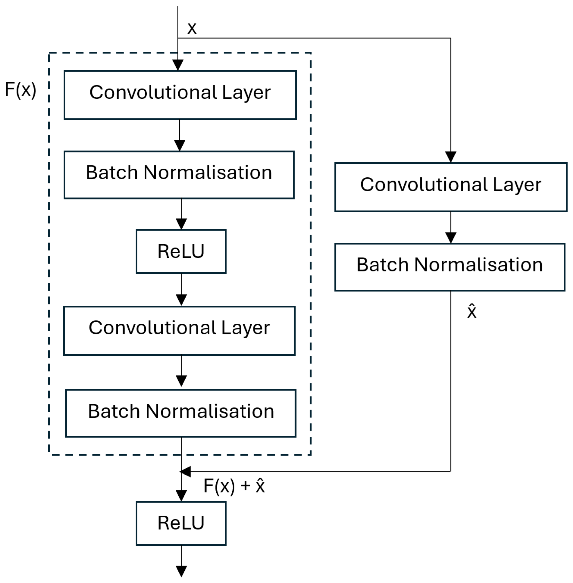
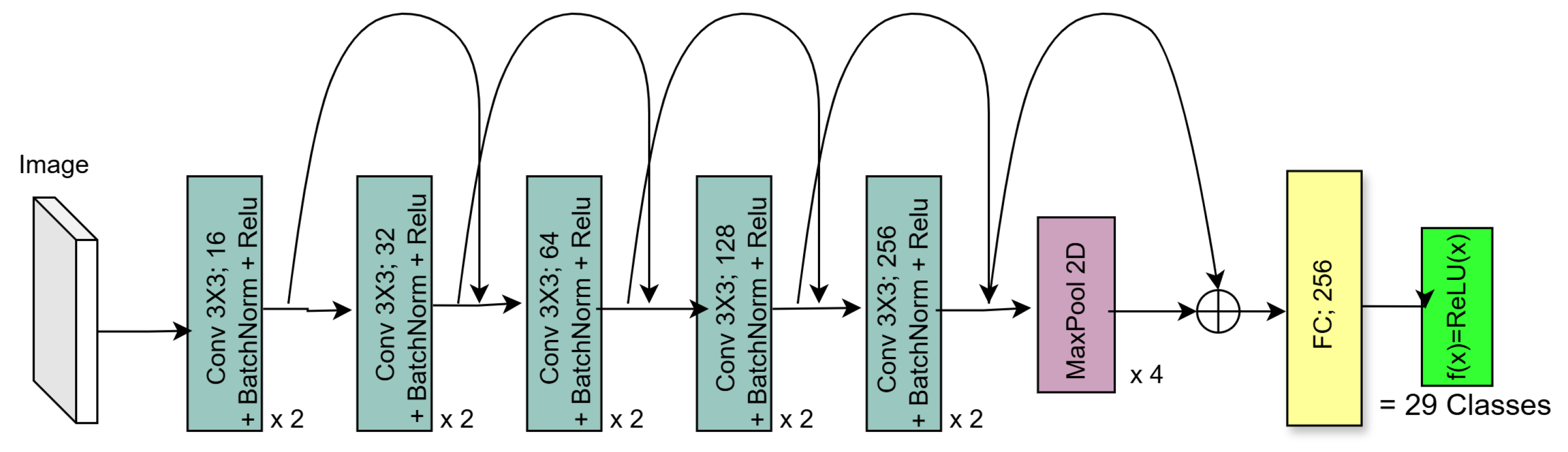
3.1. Residual Network (ResNet)
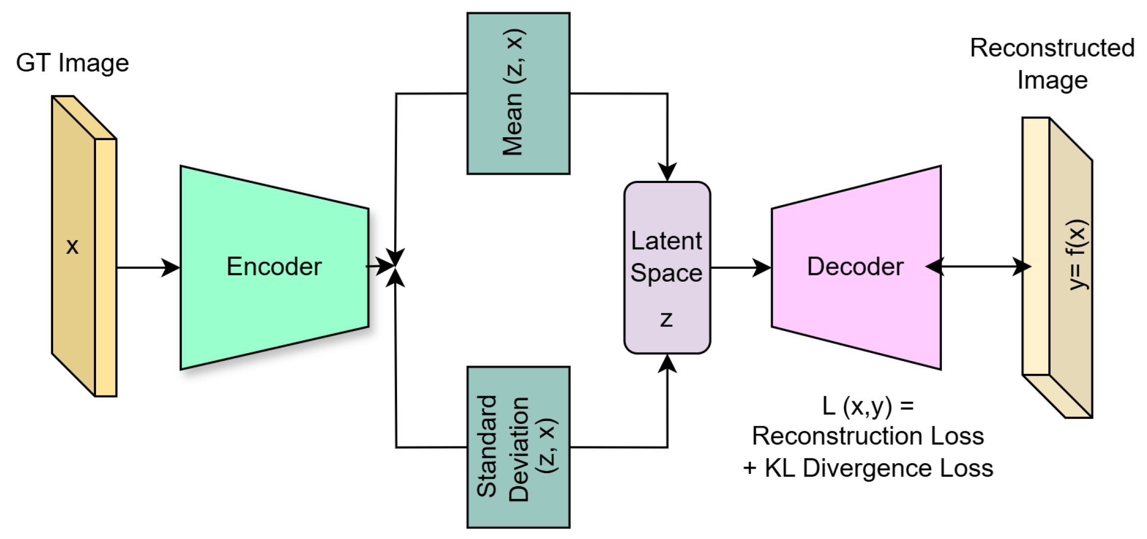
3.2. Variational Autoencoder
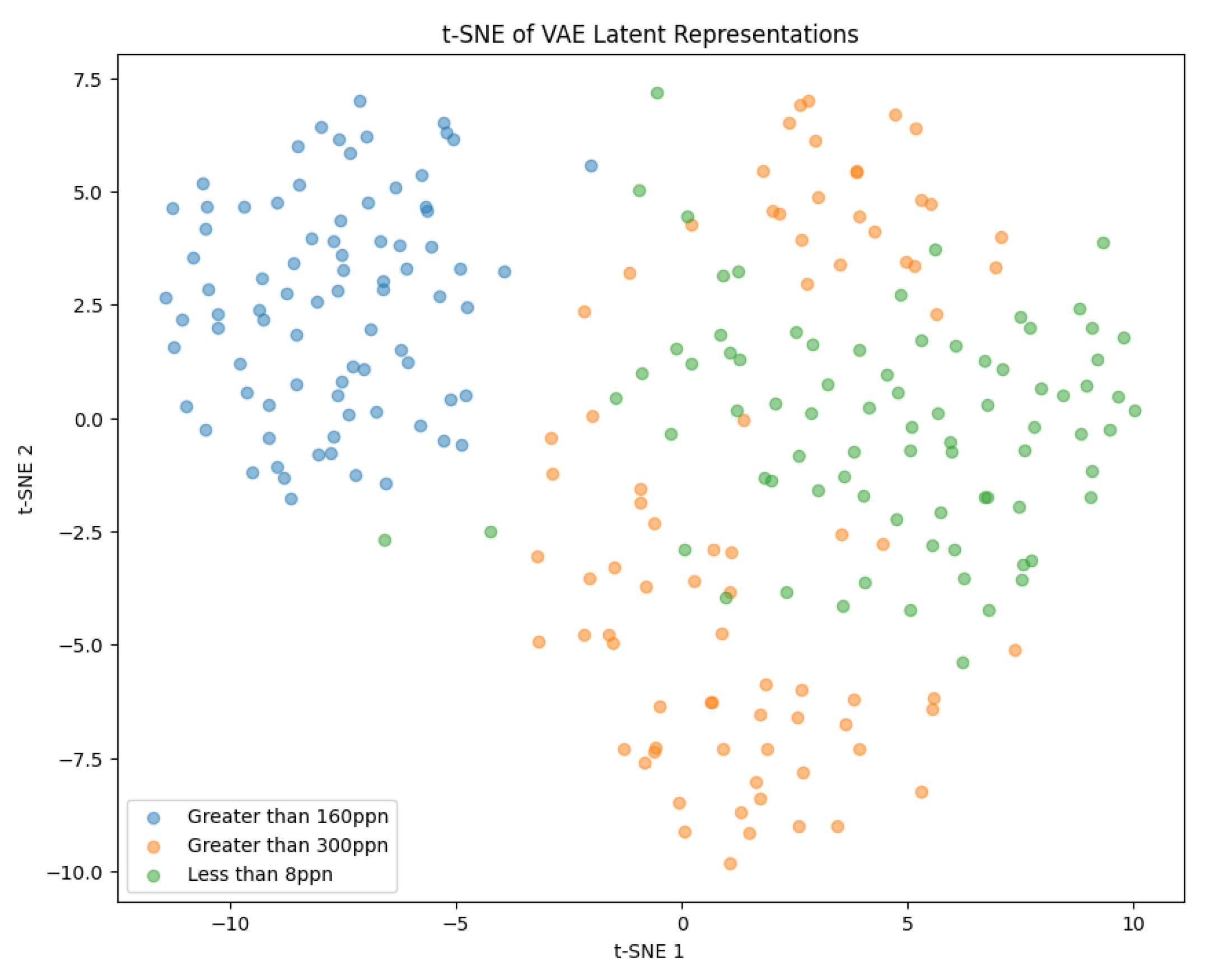
t-Distributed Stochastic Neighbor Embedding
3.3. Deep Convolutional Generative Adversarial Network
3.4. Dimensionality Reduction with K-Means Clustering
3.5. Evaluation Metrics
4. Design and Implementation
4.1. Data Processing
4.1.1. Data Format
4.1.2. Breakdown into Individual Wavelengths
4.1.3. Key Wavelength Analysis
5. Results
5.1. Dimensionality Reduction with K-Means Clustering
5.1.1. Dimensionality Reduction
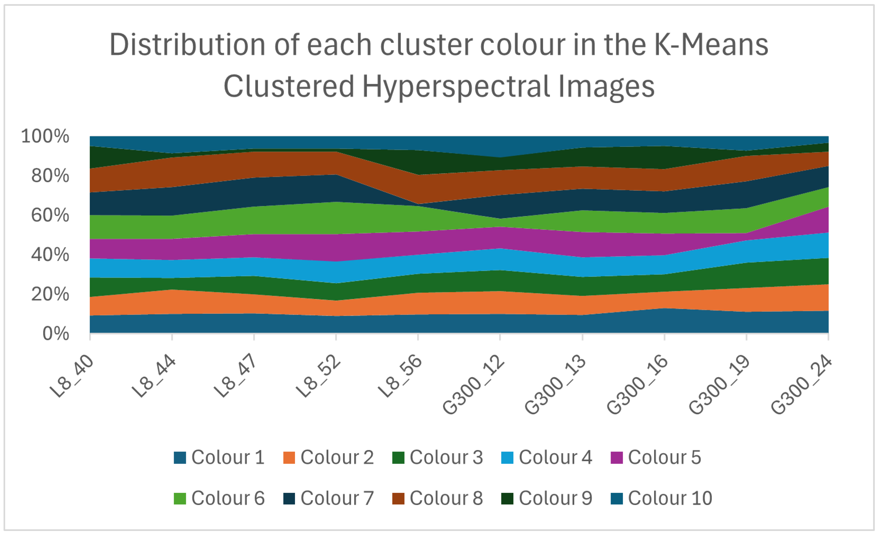
5.1.2. K-Means Clustering
5.1.3. Visual Experiment
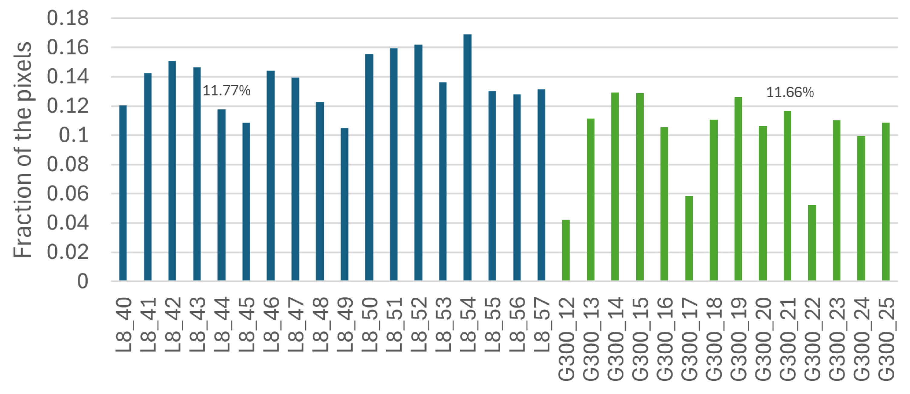
5.1.4. Pixel-by-Pixel Analysis
5.1.5. Follow-Up Experiment
5.2. Residual Network (ResNet)
5.2.1. Data Pre-Processing
5.2.2. Residual Architecture
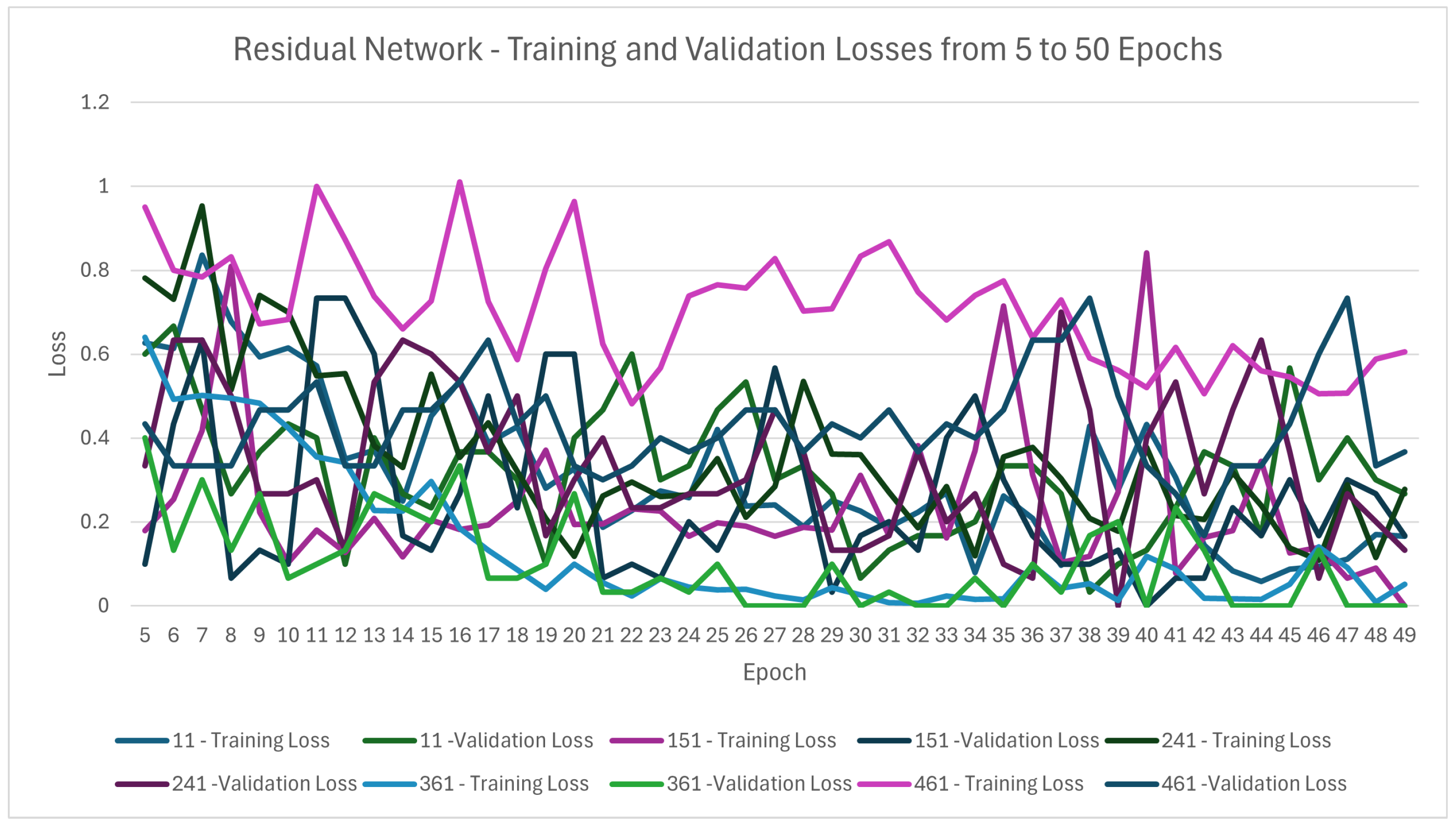
5.2.3. Results
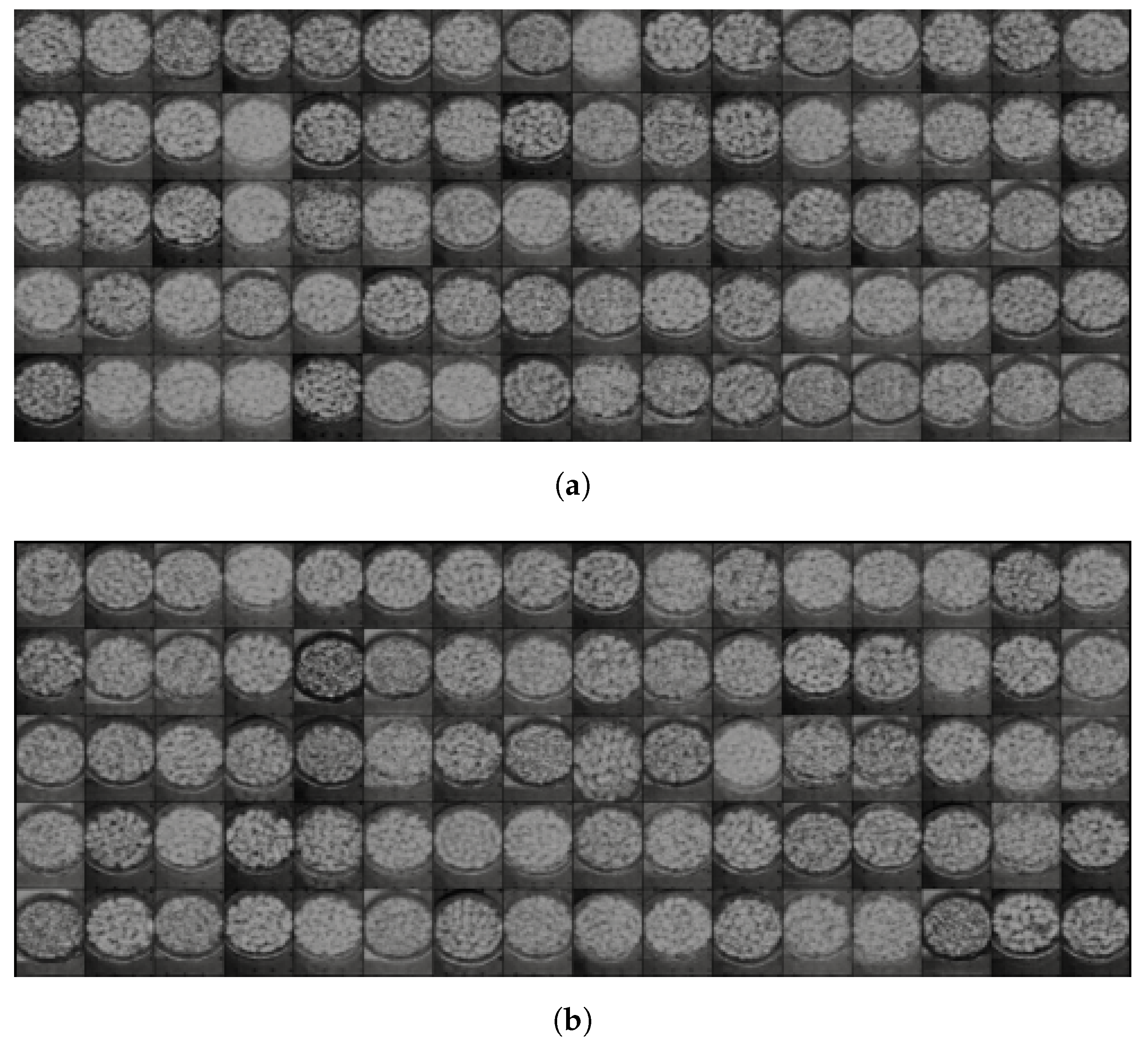
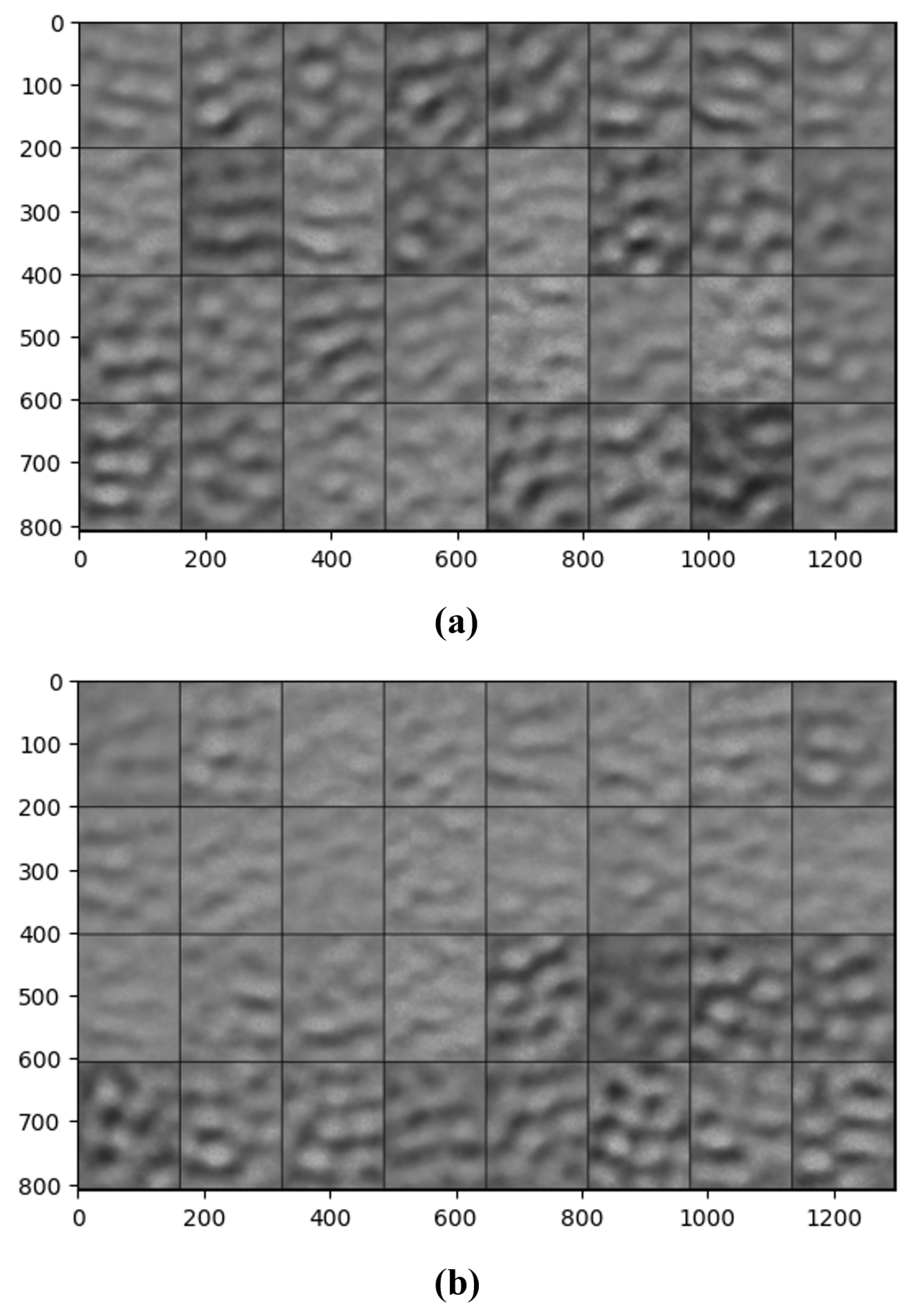
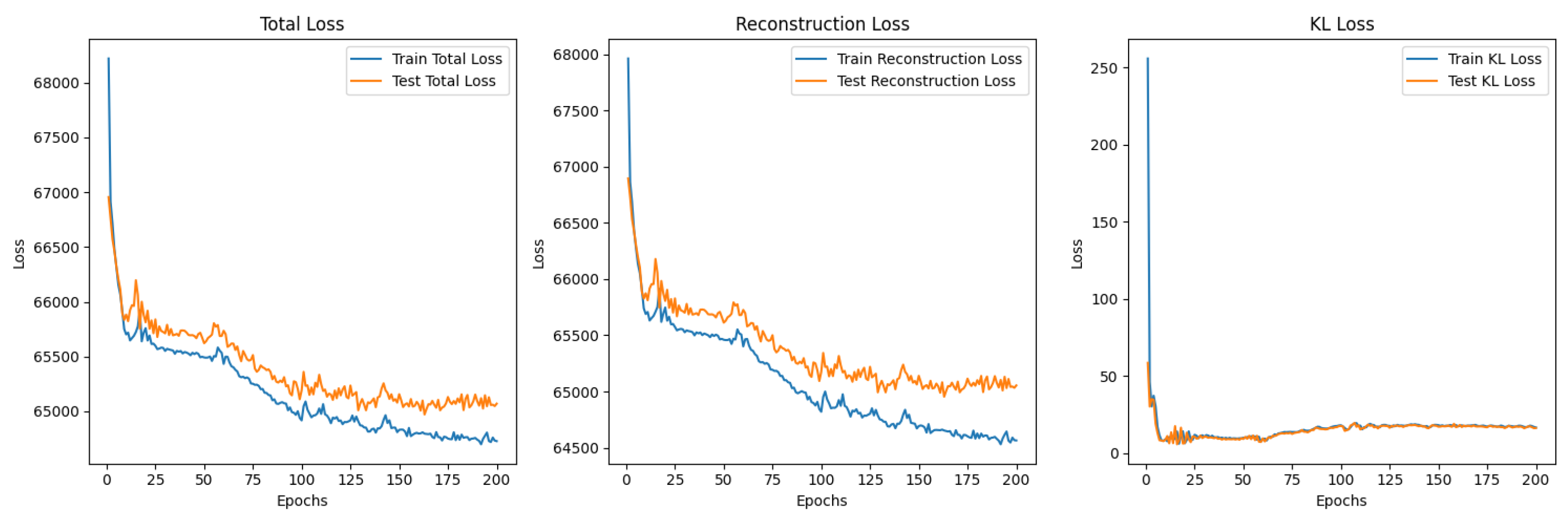
5.3. Variational Autoencoder
5.3.1. Structure of the Encoder and Decoder Networks
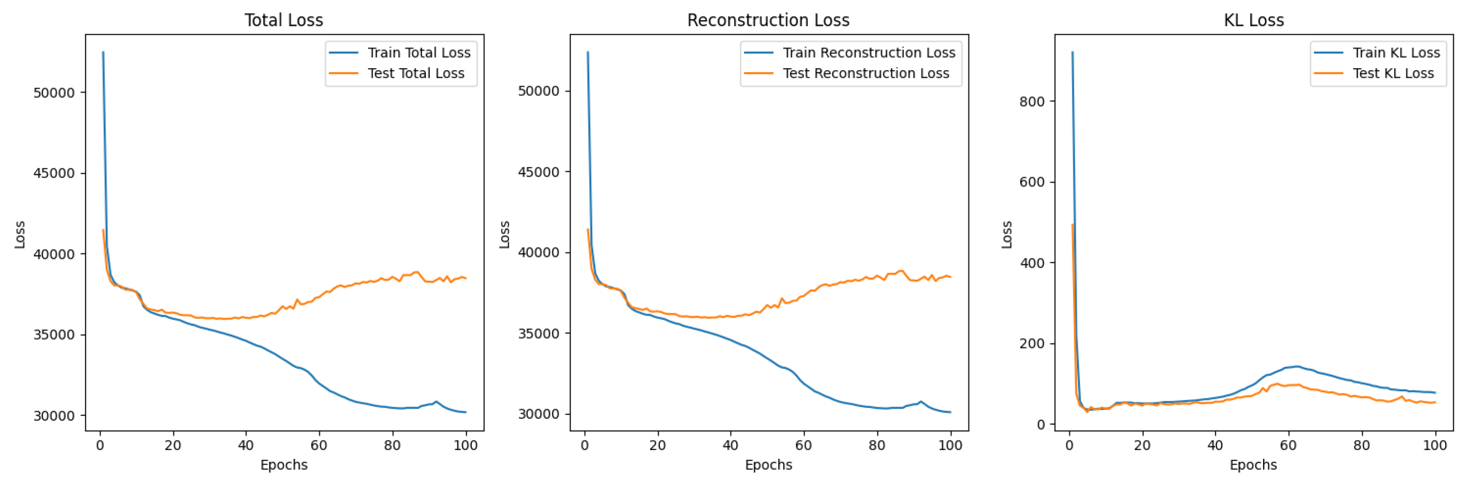
5.3.2. -Variational Autoencoder (-VAE)
5.3.3. -VAE Redesigned
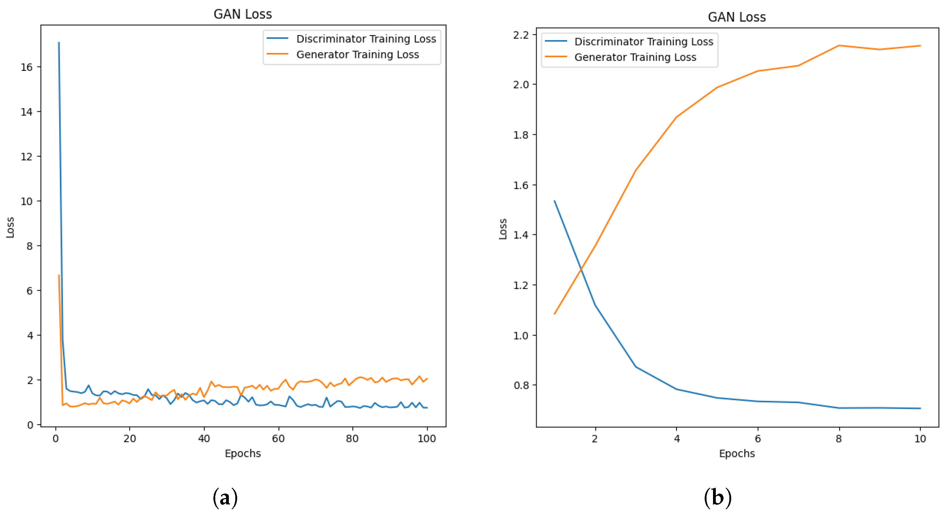
5.4. Deep Convolutional Generative Adversarial Network
5.4.1. Data Pre-Processing
5.4.2. Proposed DCGAN Structure
5.4.3. Challenges of Using DCGANs
6. Discussion
Author Contributions
Funding
Institutional Review Board Statement
Data Availability Statement
Conflicts of Interest
Abbreviations
| VAE | Variational Autoencoder |
| ResNet | Residual Network |
| DCGAN | Deep Convolutional Generative Adversarial Network |
| TLC | Thin-Layer Chromatography |
| IARC | The International Agency for Research on Cancer |
| MTL | Maximum Tolerated Level |
| HPLC | High-Performance Liquid Chromatography |
| UV | Ultra-Violet |
| LIFS | Laser-Induced Fluorescence Spectroscopy |
| PCA | Principal Component Analysis |
| LDA | Linear Discriminant Analysis |
| LRC | Logistic Regression Classification |
| SVM | Support Vector Machine |
| HSI | Hyperspectral Imagining |
| ICA | Independent Component Analysis |
| ICA-kNN | Independent Component Analysis and a K-Nearest Neighbour classifer |
| kNN | K-Nearest Neighbours |
| FDA | Fisher’s Discriminant Analysis |
| SFS | Sequential Forward Selection |
| PLS | Partial Least Squares |
| PLS-DA | Partial Least Squares-Discriminant Analysis |
| PCA-DA | Principal Component Analysis with Discriminant Analysis |
| PCA-kNN | Principal Component Analysis-based K-Nearest Neighbours |
| CART | Classification and Regression Tree |
| CNN | Convolutional Neural Network |
| t-SNE | t-Distributed Stochastic Neighbor Embedding |
| FP | False Positive |
| FN | False Negative |
| TP | True Positive |
| TN | True Negative |
| SSH | Secure Shell Protocol |
| SNR | Signal-To-Noise |
| OSP | Orthogonal Space Projection |
References
- Georgiadou, M.; Dimou, A.; Yanniotis, S. Aflatoxin contamination in pistachio nuts: A farm to storage study. Food Control 2012, 26, 580–586. [Google Scholar] [CrossRef]
- NTP (National Toxicology Program). Aflatoxins: CAS No. 1402-68-2. In Report on Carcinogens [Internet], 15th ed.; Department of Health and Human Services, Public Health Service: Research Triangle Park, NC, USA, 2021. Available online: https://ntp.niehs.nih.gov/whatwestudy/assessments/cancer/roc (accessed on 24 November 2024).
- The European Commission. Commission Regulation (EU) No 165/2010 of 26 February 2010 amending Regulation (EC) No 1881/2006 setting maximum levels for certain contaminants in foodstuffs as regards aflatoxins (Text with EEA relevance). Off. J. Eur. Union 2010, L 50, 8–12. [Google Scholar]
- Lu, R.; Chen, Y.R. Hyperspectral imaging for safety inspection of food and agricultural products. In Proceedings of the Pathogen Detection and Remediation for Safe Eating, Boston, MA, USA, 12 January 1999; Chen, Y.R., Ed.; International Society for Optics and Photonics, SPIE: Bellingham, WA, USA, 1999; Volume 3544, pp. 121–133. [Google Scholar] [CrossRef]
- Gowen, A.; O’Donnell, C.; Cullen, P.; Downey, G.; Frias, J. Hyperspectral imaging—An emerging process analytical tool for food quality and safety control. Trends Food Sci. Technol. 2007, 18, 590–598. [Google Scholar] [CrossRef]
- Kumar, V.; Singh, R.S.; Rambabu, M.; Dua, Y. Deep learning for hyperspectral image classification: A survey. Comput. Sci. Rev. 2024, 53, 100658. [Google Scholar] [CrossRef]
- Asci, S.; Devadoss, S. Trends and Issues Relevant for the US Tree Nut Sector. Choices 2021, 36, 1–7. [Google Scholar]
- Terzo, S.; Baldassano, S.; Caldara, G.F.; Ferrantelli, V.; Lo Dico, G.; Mulè, F.; Amato, A. Health benefits of pistachios consumption. Nat. Prod. Res. 2019, 33, 715–726. [Google Scholar] [CrossRef] [PubMed]
- Stroka, J.; Anklam, E. New strategies for the screening and determination of aflatoxins and the detection of aflatoxin-producing moulds in food and feed. TrAC Trends Anal. Chem. 2002, 21, 90–95. [Google Scholar] [CrossRef]
- Mokhtarian1, M.; Tavakolipour, H.; Bagheri, F.; Oliveira, C.A.F.; Corassin, C.H.; Khaneghah, A.M. Aflatoxin B1 in the Iranian pistachio nut and decontamination methods: A systematic review. Qual. Assur. Saf. Crops Foods 2020, 12, 15–25. [Google Scholar] [CrossRef]
- Cheraghali, A.; Yazdanpanah, H.; Doraki, N.; Abouhossain, G.; Hassibi, M.; Ali-abadi, S.; Aliakbarpoor, M.; Amirahmadi, M.; Askarian, A.; Fallah, N.; et al. Incidence of aflatoxins in Iran pistachio nuts. Food Chem. Toxicol. 2007, 45, 812–816. [Google Scholar] [CrossRef]
- Wall, P.; Smith, R.M. Thin-Layer Chromatography; The Royal Society of Chemistry: London, UK, 2005. [Google Scholar] [CrossRef]
- Stroka, J.; Anklam, E. Development of a simplified densitometer for the determination of aflatoxins by thin-layer chromatography. J. Chromatogr. A 2000, 904, 263–268. [Google Scholar] [CrossRef]
- Poole, C.F. Thin-layer chromatography: Challenges and opportunities. J. Chromatogr. A 2003, 1000, 963–984. [Google Scholar] [CrossRef] [PubMed]
- Blum, F. High performance liquid chromatography. Br. J. Hosp. Med. 2014, 75, C18–C21. [Google Scholar] [CrossRef] [PubMed]
- Hepsag, F.; Golge, O.; Kabak, B. Quantitation of aflatoxins in pistachios and groundnuts using HPLC-FLD method. Food Control 2014, 38, 75–81. [Google Scholar] [CrossRef]
- Wu, Q.; Xu, J.; Xu, H. Discrimination of aflatoxin B1 contaminated pistachio kernels using laser induced fluorescence spectroscopy. Biosyst. Eng. 2019, 179, 22–34. [Google Scholar] [CrossRef]
- Wu, Q.; Xu, H. Application of multiplexing fiber optic laser induced fluorescence spectroscopy for detection of aflatoxin B1 contaminated pistachio kernels. Food Chem. 2019, 290, 24–31. [Google Scholar] [CrossRef]
- Xanthopoulos, P.; Pardalos, P.M.; Trafalis, T.B. Robust Data Mining; Springer: New York, NY, USA, 2012. [Google Scholar] [CrossRef]
- Zou, X.; Hu, Y.; Tian, Z.; Shen, K. Logistic Regression Model Optimization and Case Analysis. In Proceedings of the 2019 IEEE 7th International Conference on Computer Science and Network Technology (ICCSNT), Dalian, China, 19–20 October 2019; pp. 135–139. [Google Scholar] [CrossRef]
- Khan, M.J.; Khan, H.S.; Yousaf, A.; Khurshid, K.; Abbas, A. Modern Trends in Hyperspectral Image Analysis: A Review. IEEE Access 2018, 6, 14118–14129. [Google Scholar] [CrossRef]
- Grahn, H.; Geladi, P. Techniques and Applications of Hyperspectral Image Analysis; John Wiley & Sons, Ltd.: Hoboken, NJ, USA, 2007. [Google Scholar]
- Lodhi, V.; Chakravarty, D.; Mitra, P. Hyperspectral Imaging System: Development Aspects and Recent Trends. Sens. Imaging 2019, 20, 35. [Google Scholar] [CrossRef]
- Ndu, H.; Sheikh-Akbari, A.; Deng, J.; Mporas, I. HyperVein: A Hyperspectral Image Dataset for Human Vein Detection. Sensors 2024, 24, 1118. [Google Scholar] [CrossRef]
- Moghaddam, T.M.; Razavi, S.M.A.; Taghizadeh, M. Applications of hyperspectral imaging in grains and nuts quality and safety assessment: A review. J. Food Meas. Charact. 2013, 7, 129–140. [Google Scholar] [CrossRef]
- Zhu, B.; Jiang, L.; Jin, F.; Qin, L.; Vogel, A.; Tao, Y. Walnut shell and meat differentiation using fluorescence hyperspectral imagery with ICA-kNN optimal wavelength selection. Sens. Instrum. Food Qual. Saf. 2007, 1, 123–131. [Google Scholar] [CrossRef]
- Jiang, L.; Zhu, B.; Rao, X.; Berney, G.; Tao, Y. Discrimination of black walnut shell and pulp in hyperspectral fluorescence imagery using Gaussian kernel function approach. J. Food Eng. 2007, 81, 108–117. [Google Scholar] [CrossRef]
- Nakariyakul, S.; Casasent, D.P. Classification of internally damaged almond nuts using hyperspectral imagery. J. Food Eng. 2011, 103, 62–67. [Google Scholar] [CrossRef]
- Bonifazi, G.; Capobianco, G.; Gasbarrone, R.; Serranti, S. Contaminant detection in pistachio nuts by different classification methods applied to short-wave infrared hyperspectral images. Food Control 2021, 130, 108202. [Google Scholar] [CrossRef]
- Szymańska, E.; Saccenti, E.; Smilde, A.K.; Westerhuis, J.A. Double-check: Validation of diagnostic statistics for PLS-DA models in metabolomics studies. Metabolomics 2011, 8, 3–16. [Google Scholar] [CrossRef]
- Brown, M.T.; Wicker, L.R. 8-Discriminant Analysis. In Handbook of Applied Multivariate Statistics and Mathematical Modeling; Tinsley, H.E., Brown, S.D., Eds.; Academic Press: San Diego, CA, USA, 2000; pp. 209–235. [Google Scholar] [CrossRef]
- Capobianco, G.; Bracciale, M.P.; Sali, D.; Sbardella, F.; Belloni, P.; Bonifazi, G.; Serranti, S.; Santarelli, M.L.; Cestelli Guidi, M. Chemometrics approach to FT-IR hyperspectral imaging analysis of degradation products in artwork cross-section. Microchem. J. 2017, 132, 69–76. [Google Scholar] [CrossRef]
- Laaksonen, J.; Oja, E. Classification with learning k-nearest neighbors. In Proceedings of the International Conference on Neural Networks (ICNN’96), Washington, DC, USA, 3–6 June 1996; Volume 3, pp. 1480–1483. [Google Scholar] [CrossRef]
- Lewis, R.J. An Introduction to Classification and Regression Tree (CART) Analysis. In Proceedings of the 2000 Annual Meeting of the Society for Academic Emergency Medicine, San Francisco, CA, USA, 22–25 May 2000. [Google Scholar]
- O’Shea, K.; Nash, R. An Introduction to Convolutional Neural Networks. arXiv 2015, arXiv:1511.08458. [Google Scholar]
- He, K.; Zhang, X.; Ren, S.; Sun, J. Deep Residual Learning for Image Recognition. In Proceedings of the 2016 IEEE Conference on Computer Vision and Pattern Recognition (CVPR), Las Vegas, NV, USA, 27–30 June 2016; pp. 770–778. [Google Scholar] [CrossRef]
- An, R.; Perez-Cruet, J.; Wang, J. We got nuts! use deep neural networks to classify images of common edible nuts. Nutr. Health 2024, 30, 301–307. [Google Scholar] [CrossRef] [PubMed]
- Zhong, Z.; Li, J.; Ma, L.; Jiang, H.; Zhao, H. Deep residual networks for hyperspectral image classification. In Proceedings of the 2017 IEEE International Geoscience and Remote Sensing Symposium (IGARSS), Fort Worth, TX, USA, 23–28 July 2017; pp. 1824–1827. [Google Scholar] [CrossRef]
- GM, H.; Gourisaria, M.K.; Pandey, M.; Rautaray, S.S. A comprehensive survey and analysis of generative models in machine learning. Comput. Sci. Rev. 2020, 38, 100285. [Google Scholar] [CrossRef]
- Bergamin, L.; Carraro, T.; Polato, M.; Aiolli, F. Novel Applications for VAE-based Anomaly Detection Systems. In Proceedings of the 2022 International Joint Conference on Neural Networks (IJCNN), Padua, Italy, 18–23 July 2022; pp. 1–8. [Google Scholar] [CrossRef]
- van der Maaten, L.; Hinton, G. Visualizing Data using t-SNE. J. Mach. Learn. Res. 2008, 9, 2579–2605. [Google Scholar]
- Dey, P.; Saurabh, K.; Kumar, C.; Pandit, D.; Chaulya, S.K.; Ray, S.K.; Prasad, G.M.; Mandal, S.K. t-SNE and variational auto-encoder with a bi-LSTM neural network-based model for prediction of gas concentration in a sealed-off area of underground coal mines. Soft Comput. 2021, 25, 14183–14207. [Google Scholar] [CrossRef]
- Mahmoud, M.A.B.; Guo, P.; Wang, K. Pseudoinverse learning autoencoder with DCGAN for plant diseases classification. Multimed. Tools Appl. 2020, 79, 26245–26263. [Google Scholar] [CrossRef]
- Tan, H.; Hu, Y.; Ma, B.; Yu, G.; Li, Y. An improved DCGAN model: Data augmentation of hyperspectral image for identification pesticide residues of Hami melon. Food Control 2024, 157, 110168. [Google Scholar] [CrossRef]
- Pakhira, M.K. A Linear Time-Complexity k-Means Algorithm Using Cluster Shifting. In Proceedings of the 2014 International Conference on Computational Intelligence and Communication Networks, CICN ’14, Orlando, FL, USA, 9–12 December 2014; pp. 1047–1051. [Google Scholar] [CrossRef]
- Kodinariya, T.M.; Makwana, P.R. Review on determining number of Cluster in K-Means Clustering. Int. J. 2013, 1, 90–95. [Google Scholar]
- Zhu, H.; Zhao, Y.; Yang, L.; Zhao, L.; Han, Z. Pixel-level deep spectral features and unsupervised learning for detecting aflatoxin B1 on peanut kernels. Postharvest Biol. Technol. 2023, 202, 112376. [Google Scholar] [CrossRef]
- Du, Q.; Yang, H. Similarity-Based Unsupervised Band Selection for Hyperspectral Image Analysis. IEEE Geosci. Remote Sens. Lett. 2008, 5, 564–568. [Google Scholar] [CrossRef]


| Metric | Value |
|---|---|
| Accuracy | |
| Precision | |
| Recall | |
| F1-Score |
| True Aflatoxin Level | Total | |||
|---|---|---|---|---|
| Less Than 8 | Greater Than 300 | |||
| Prediction | Less Than 8 | 16 | 3 | 19 |
| Greater Than 300 | 2 | 11 | 13 | |
| Total | 18 | 14 | 32 | |
| True Aflatoxin Level | Total | ||||
|---|---|---|---|---|---|
| L8 | G160 | G300 | |||
| Prediction | L8 | 10 | 0 | 0 | 10 |
| G160 | 0 | 10 | 0 | 10 | |
| G300 | 0 | 0 | 10 | 10 | |
| Total | 10 | 10 | 10 | 30 | |
| True Aflatoxin Level | Total | ||||
|---|---|---|---|---|---|
| L8 | G160 | G300 | |||
| Prediction | L8 | 10 | 0 | 0 | 10 |
| G160 | 0 | 9 | 1 | 10 | |
| G300 | 0 | 0 | 10 | 10 | |
| Total | 10 | 9 | 11 | 30 | |
| Metric | Value |
|---|---|
| Accuracy | |
| Precision | |
| Precision | |
| Precision | |
| Recall | |
| Recall | |
| Recall | |
| F1-Score | |
| F1-Score | |
| F1-Score |
Disclaimer/Publisher’s Note: The statements, opinions and data contained in all publications are solely those of the individual author(s) and contributor(s) and not of MDPI and/or the editor(s). MDPI and/or the editor(s) disclaim responsibility for any injury to people or property resulting from any ideas, methods, instructions or products referred to in the content. |
© 2025 by the authors. Licensee MDPI, Basel, Switzerland. This article is an open access article distributed under the terms and conditions of the Creative Commons Attribution (CC BY) license (https://creativecommons.org/licenses/by/4.0/).
Share and Cite
Williams, L.; Shukla, P.; Sheikh-Akbari, A.; Mahroughi, S.; Mporas, I. Measuring the Level of Aflatoxin Infection in Pistachio Nuts by Applying Machine Learning Techniques to Hyperspectral Images. Sensors 2025, 25, 1548. https://doi.org/10.3390/s25051548
Williams L, Shukla P, Sheikh-Akbari A, Mahroughi S, Mporas I. Measuring the Level of Aflatoxin Infection in Pistachio Nuts by Applying Machine Learning Techniques to Hyperspectral Images. Sensors. 2025; 25(5):1548. https://doi.org/10.3390/s25051548
Chicago/Turabian StyleWilliams, Lizzie, Pancham Shukla, Akbar Sheikh-Akbari, Sina Mahroughi, and Iosif Mporas. 2025. "Measuring the Level of Aflatoxin Infection in Pistachio Nuts by Applying Machine Learning Techniques to Hyperspectral Images" Sensors 25, no. 5: 1548. https://doi.org/10.3390/s25051548
APA StyleWilliams, L., Shukla, P., Sheikh-Akbari, A., Mahroughi, S., & Mporas, I. (2025). Measuring the Level of Aflatoxin Infection in Pistachio Nuts by Applying Machine Learning Techniques to Hyperspectral Images. Sensors, 25(5), 1548. https://doi.org/10.3390/s25051548