
The Performance of an ML-Based Weigh-in-Motion System in the Context of a Network Arch Bridge Structural Specificity


Abstract
1. Introduction
2. Methodology
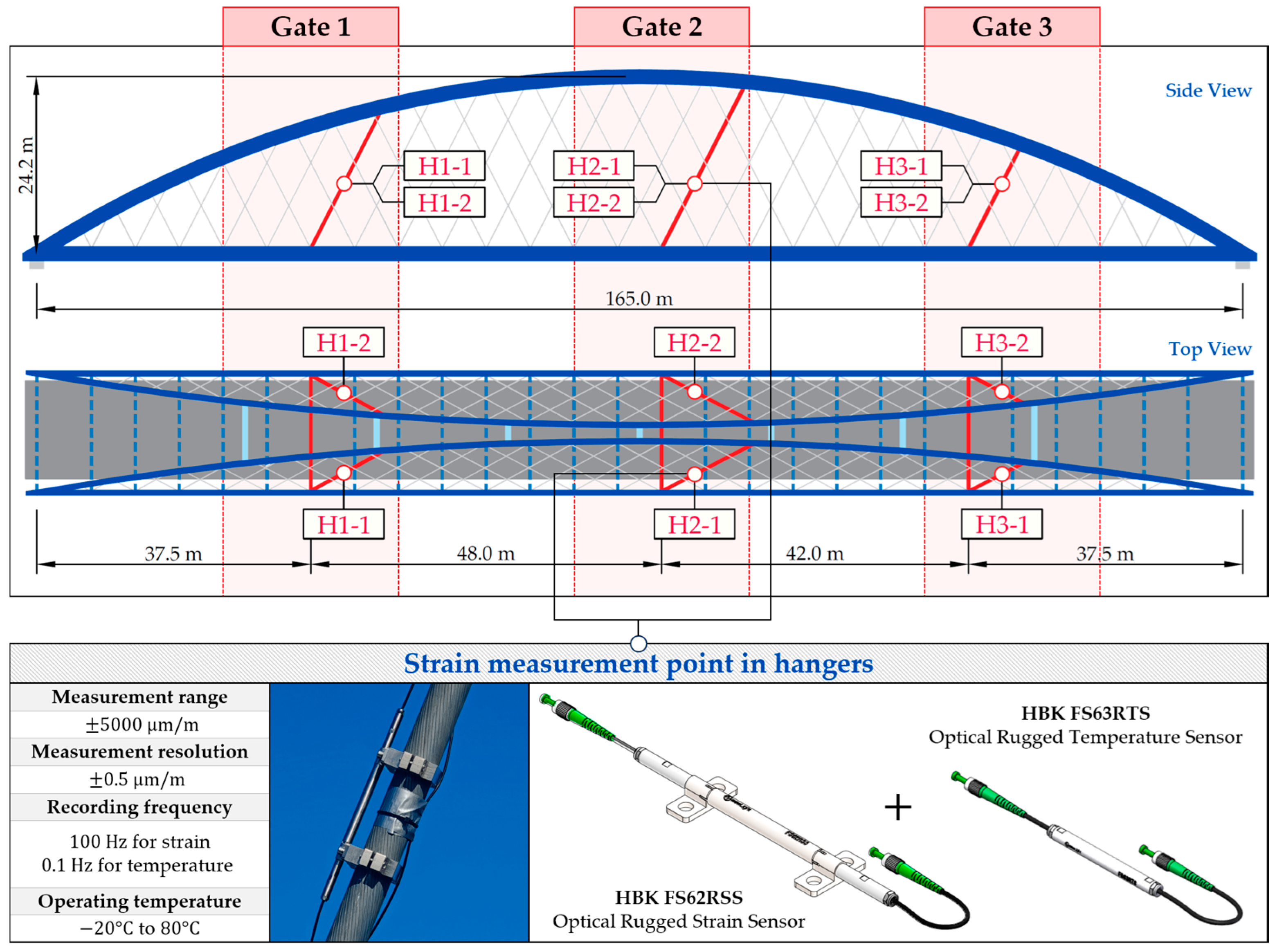
2.1. Bridge and SHM System Overview
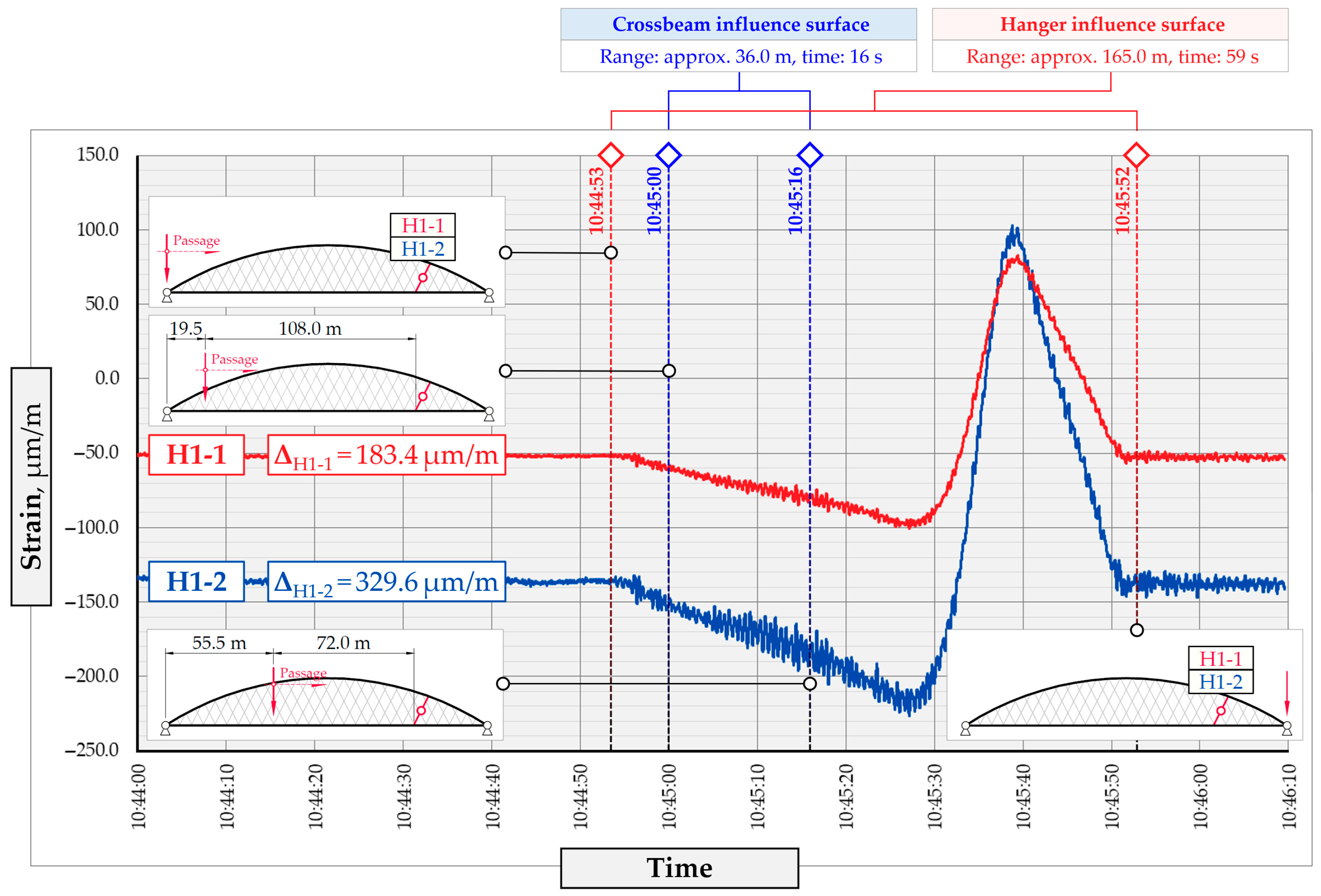
2.2. Load Testing and Physics-Informed BWIM Design
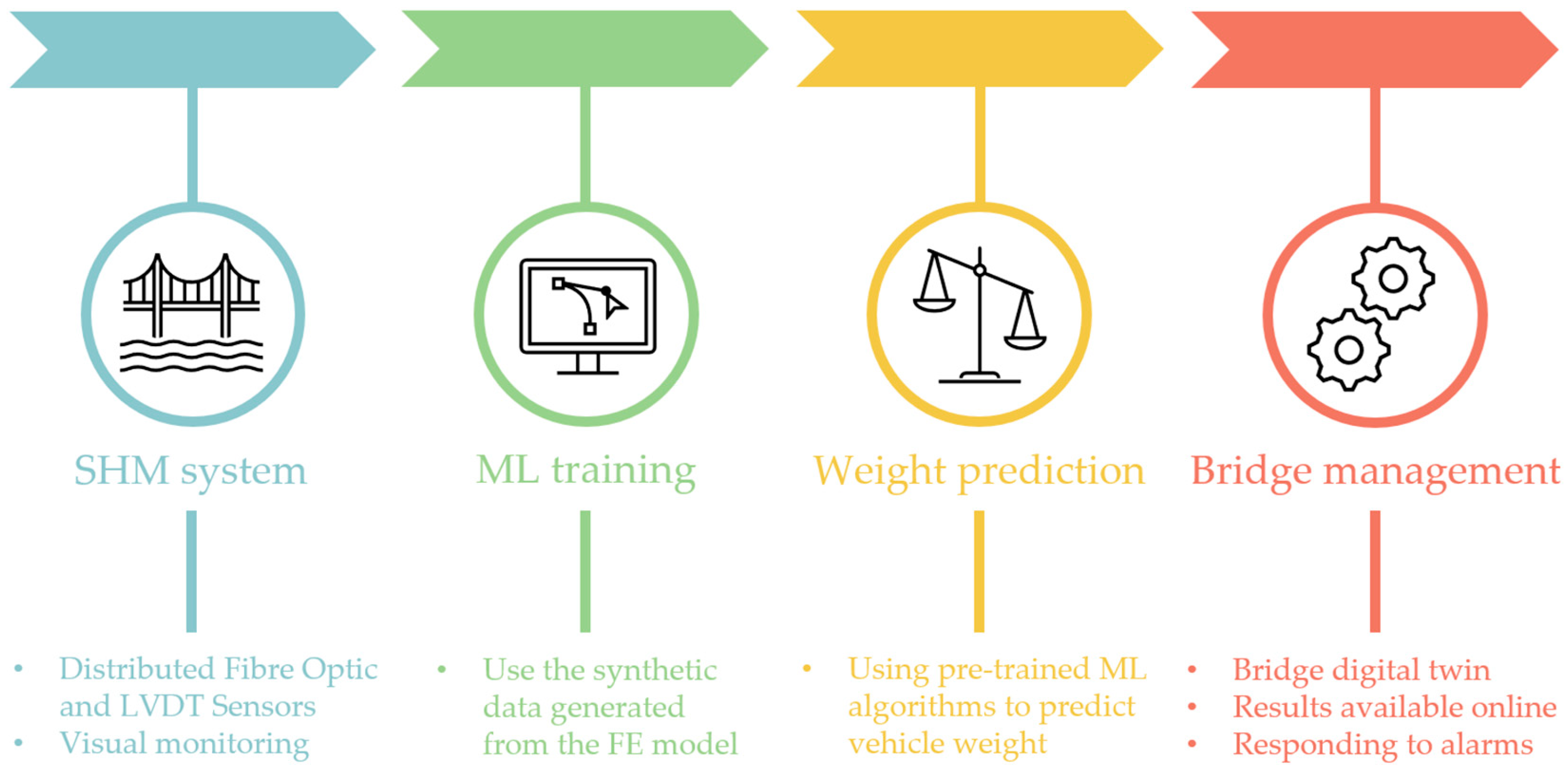
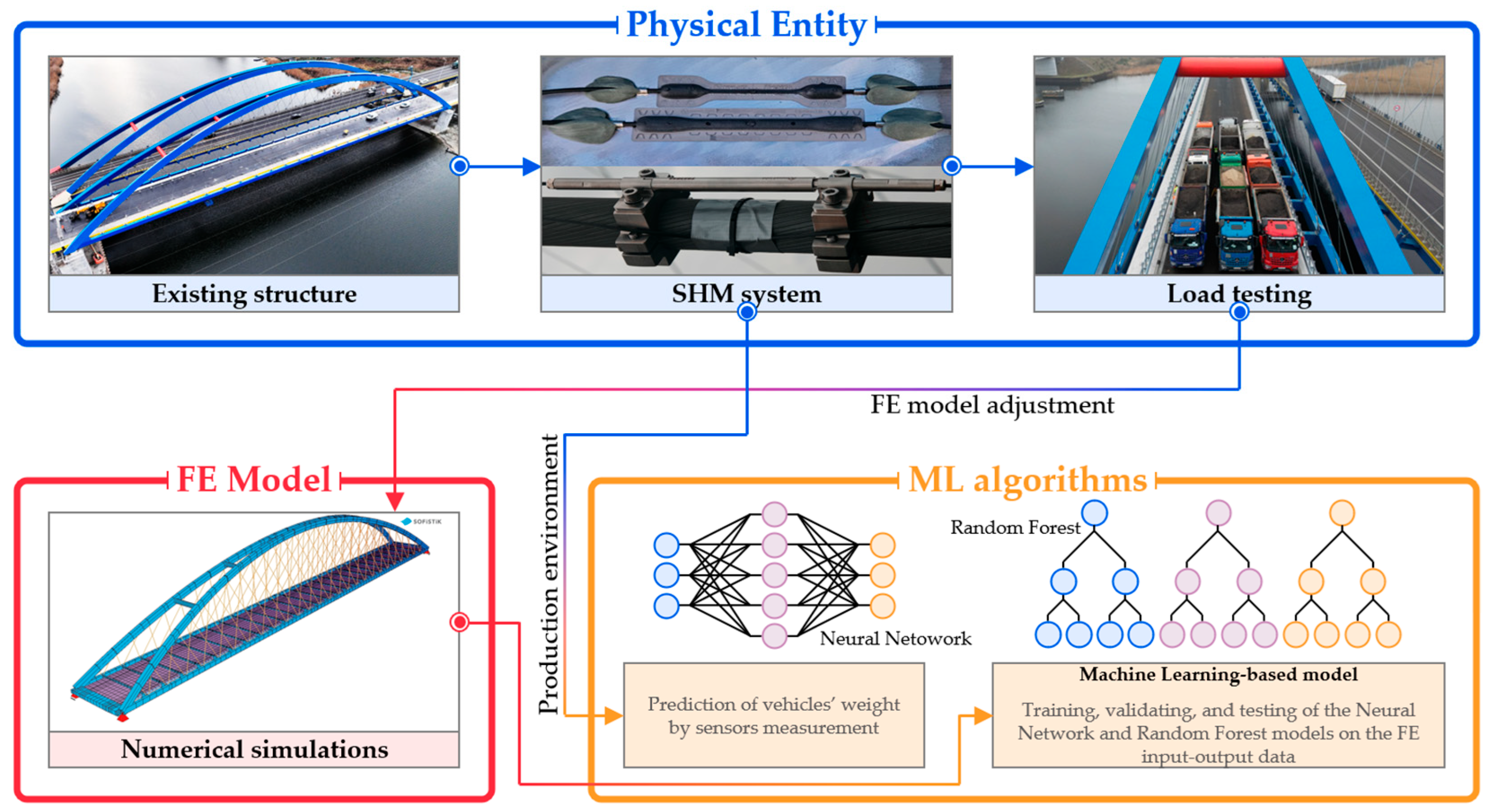
2.3. Methods and Further Use
3. Results
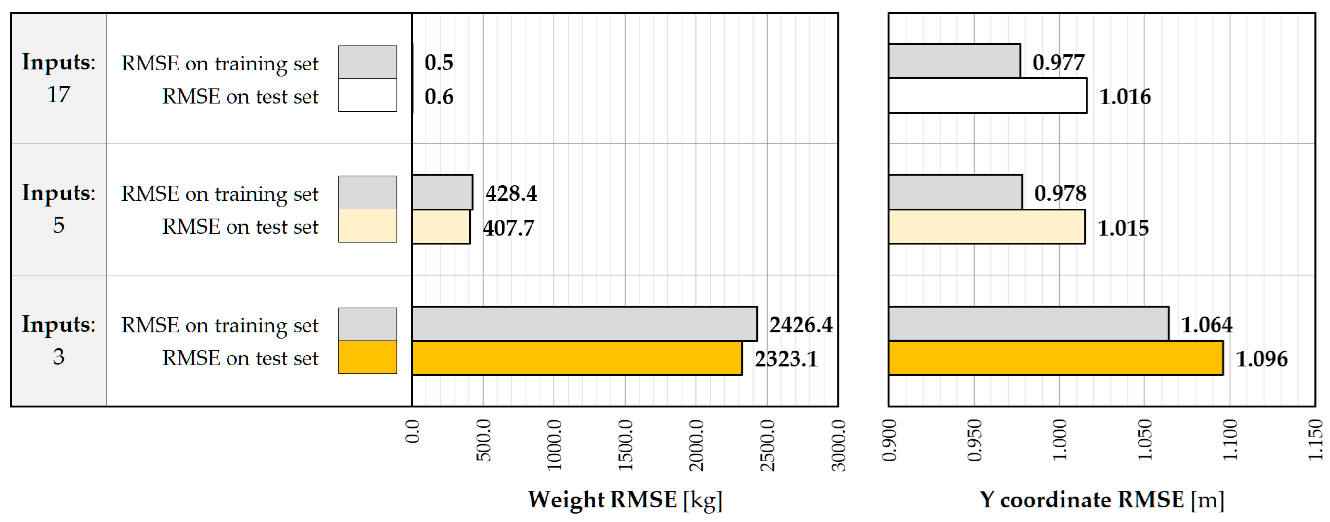
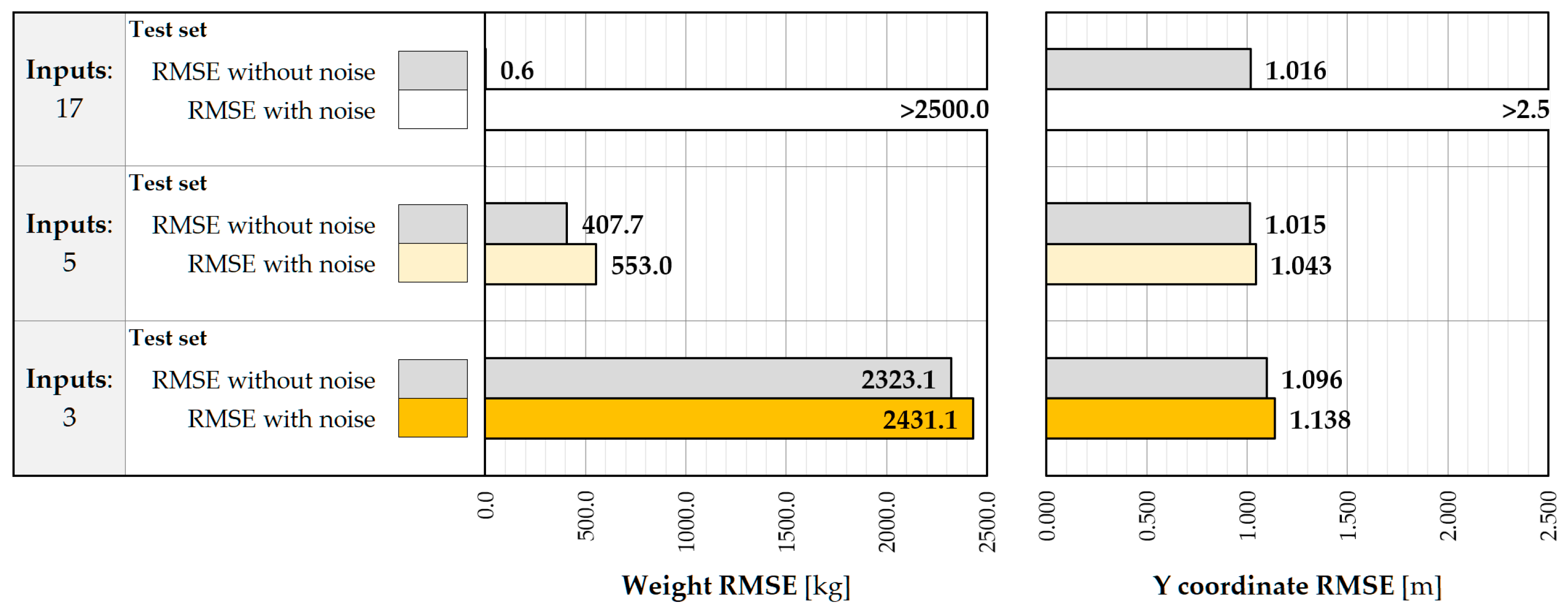
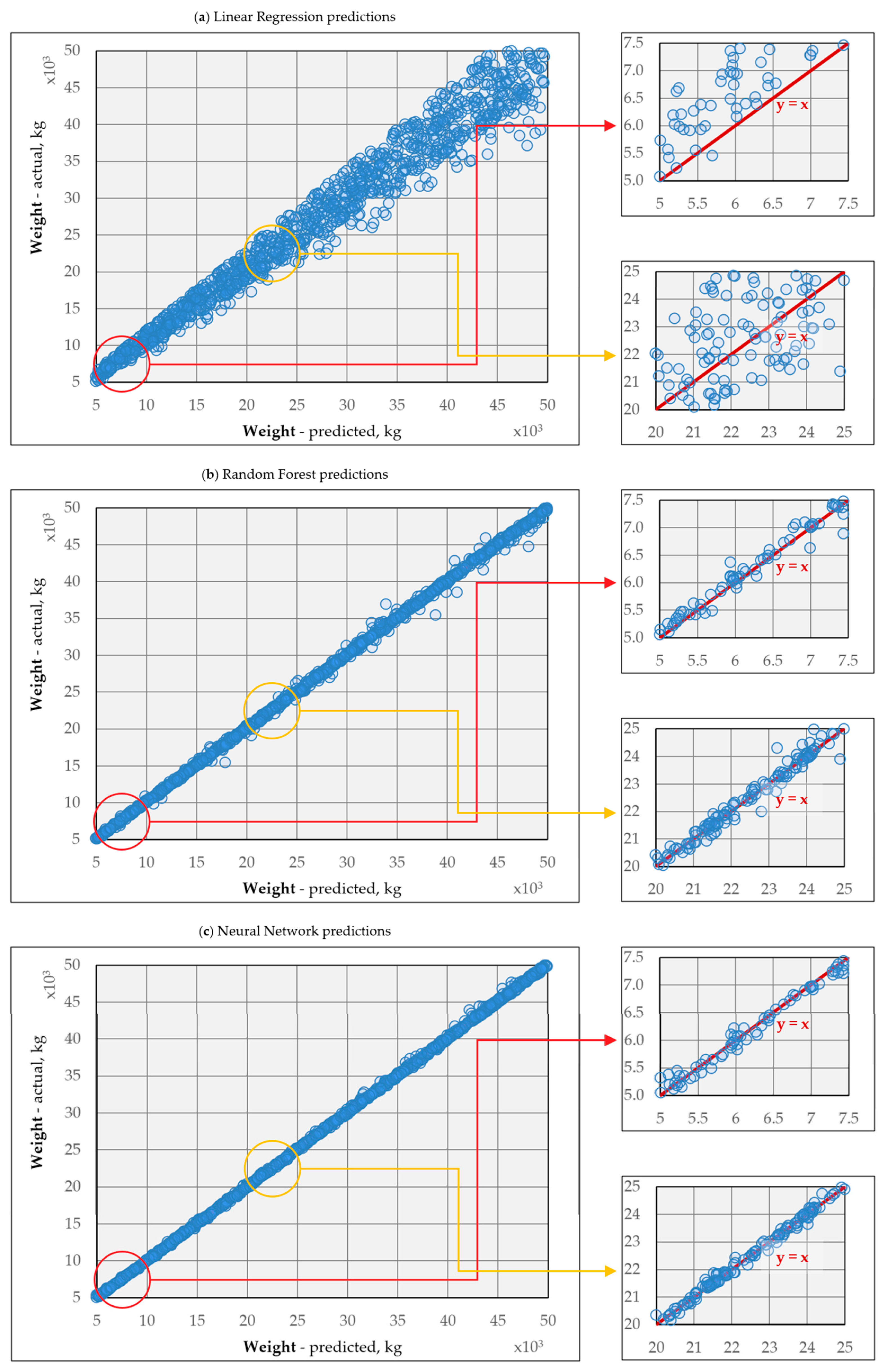
3.1. Linear Regression-Based Predictive Models
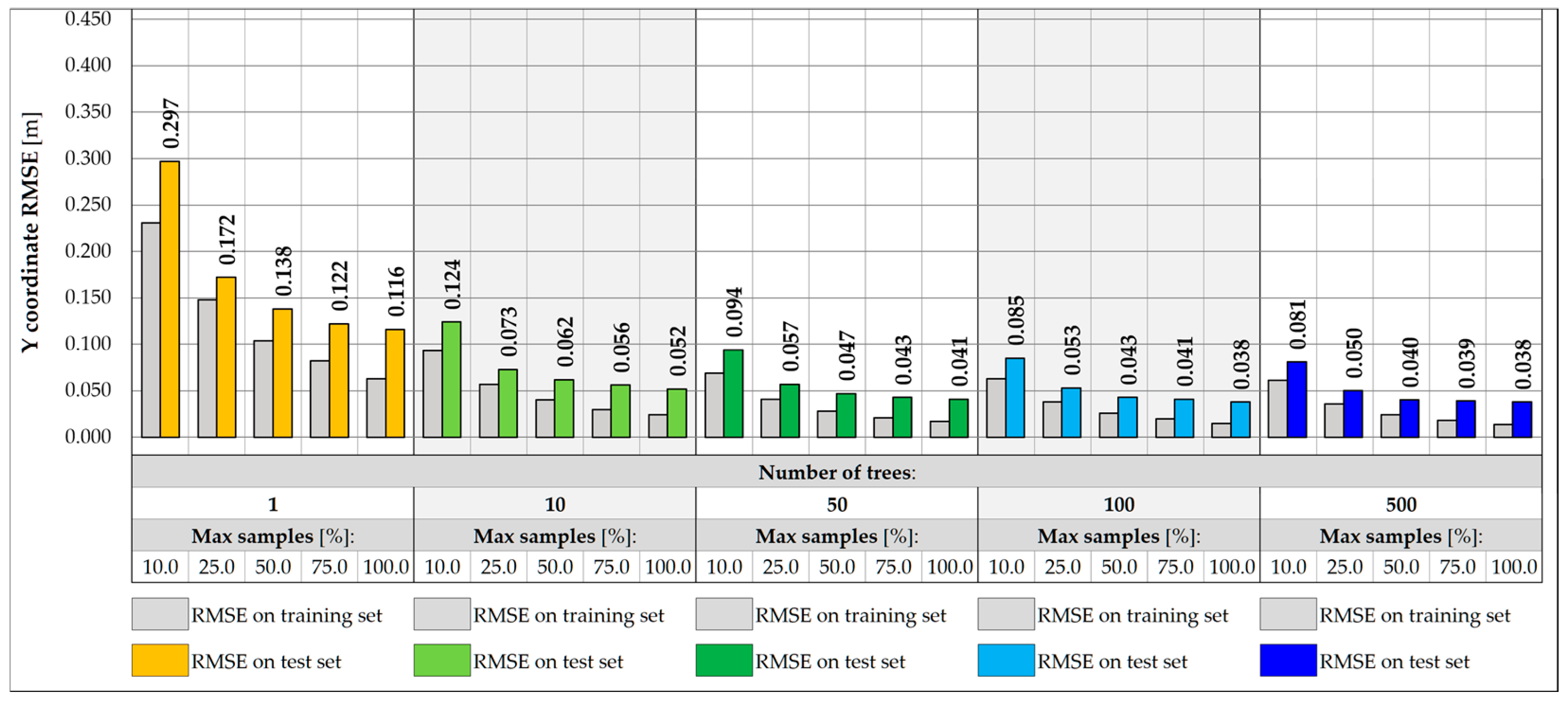
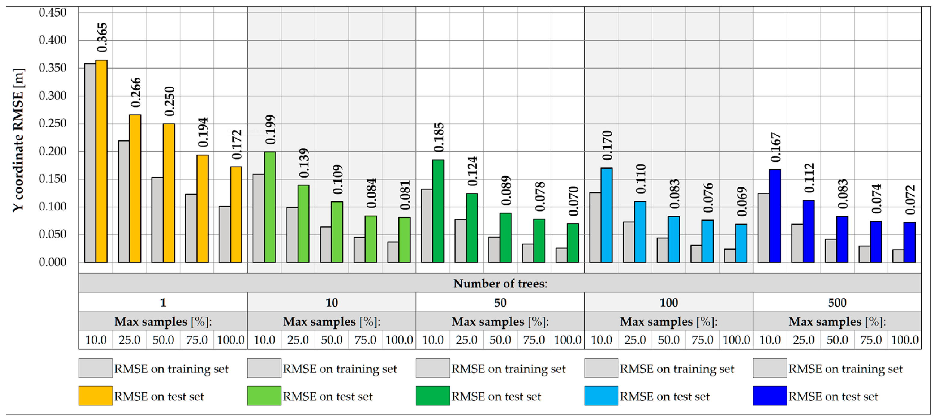
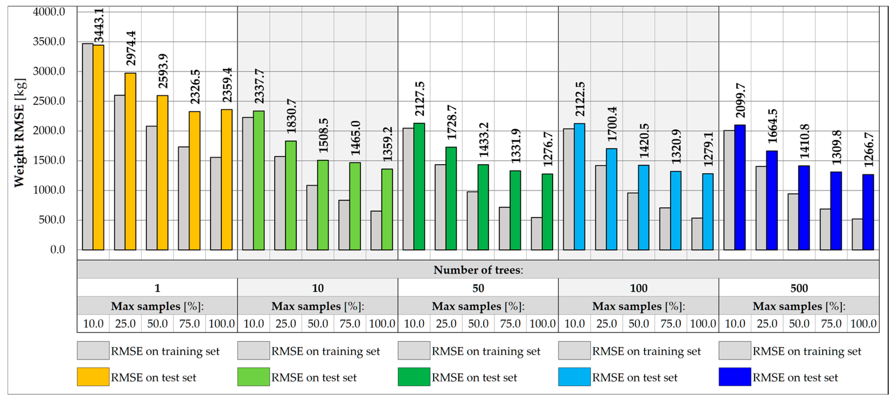
3.2. Random Forest-Based Predictive Models
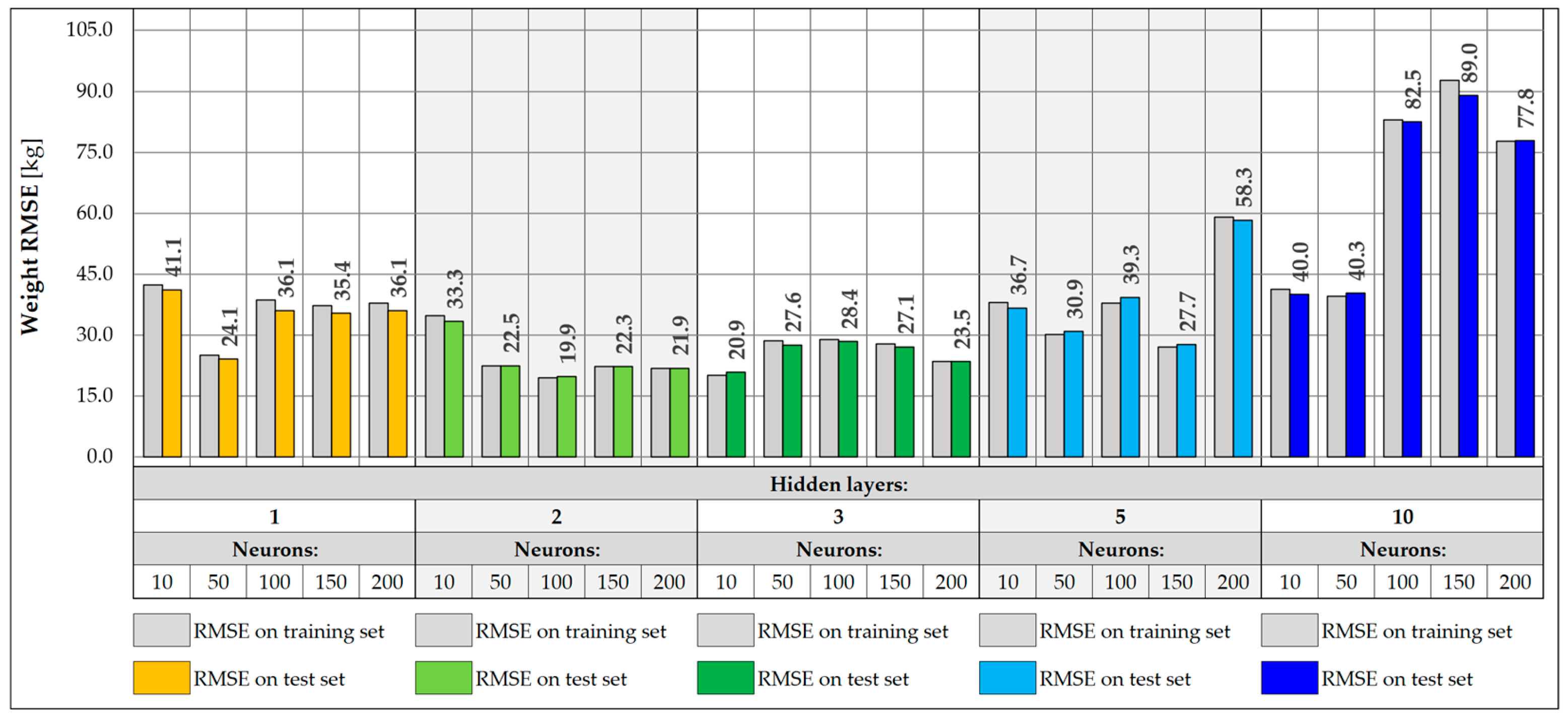
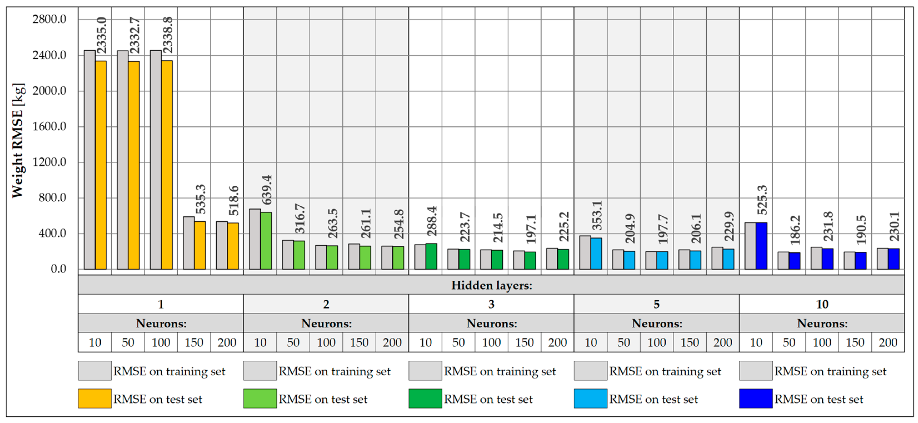
3.3. Neural Network-Based Predictive Models
3.4. Model Accuracy
4. Conclusions
Author Contributions
Funding
Institutional Review Board Statement
Informed Consent Statement
Data Availability Statement
Conflicts of Interest
References
- Pozo, F.; Tibaduiza, D.A.; Vidal, Y. Sensors for Structural Health Monitoring and Condition Monitoring. Sensors 2021, 21, 1558. [Google Scholar] [CrossRef] [PubMed]
- Moser, D.; Martin-Candilejo, A.; Cueto-Felgueroso, L.; Santillán, D. Use of Fiber-Optic Sensors to Monitor Concrete Dams: Recent Breakthroughs and New Opportunities. Structures 2024, 67, 106968. [Google Scholar] [CrossRef]
- Richter, B.; Messerer, D.; Herbers, M.; Speck, K.; Laukner, J.; Gläser, C.; Jesse, F.; Marx, S. Monitoring of a Prestressed Bridge Girder with Integrated Distributed Fiber Optic Sensors. Procedia Struct. Integr. 2024, 64, 1208–1215. [Google Scholar] [CrossRef]
- Li, H.-J.; Zhu, H.-H.; Wu, H.-Y.; Zhu, B.; Shi, B. Experimental Investigation on Pipe-Soil Interaction Due to Ground Subsidence via High-Resolution Fiber Optic Sensing. Tunn. Undergr. Space Technol. 2022, 127, 104586. [Google Scholar] [CrossRef]
- Ren, B.; Zhu, H.; Shen, Y.; Zhou, X.; Zhao, T. Deformation Monitoring of Ultra-Deep Foundation Excavation Using Distributed Fiber Optic Sensors. IOP Conf. Ser. Earth Env. Sci. 2021, 861, 072057. [Google Scholar] [CrossRef]
- García, I.; Zubia, J.; Durana, G.; Aldabaldetreku, G.; Illarramendi, M.; Villatoro, J. Optical Fiber Sensors for Aircraft Structural Health Monitoring. Sensors 2015, 15, 15494–15519. [Google Scholar] [CrossRef]
- Bae, C.; Manandhar, A.; Kiesel, P.; Raghavan, A. Monitoring the Strain Evolution of Lithium-Ion Battery Electrodes Using an Optical Fiber Bragg Grating Sensor. Energy Technol. 2016, 4, 851–855. [Google Scholar] [CrossRef]
- Ikeda, Y.; Takeda, S.; Hisada, S.; Ogasawara, T. Detection of Matrix Cracks in Composite Laminates Using Embedded Fiber-Optic Distributed Strain Sensing. Sens. Actuators A Phys. 2024, 380, 116039. [Google Scholar] [CrossRef]
- Wang, H.; Jiang, L.; Xiang, P. Improving the Durability of the Optical Fiber Sensor Based on Strain Transfer Analysis. Opt. Fiber Technol. 2018, 42, 97–104. [Google Scholar] [CrossRef]
- Khonina, S.N.; Kazanskiy, N.L.; Butt, M.A. Optical Fibre-Based Sensors—An Assessment of Current Innovations. Biosensors 2023, 13, 835. [Google Scholar] [CrossRef]
- Al-Tarawneh, M.; Huang, Y.; Lu, P.; Bridgelall, R. Weigh-In-Motion System in Flexible Pavements Using Fiber Bragg Grating Sensors Part A: Concept. IEEE Trans. Intell. Transp. Syst. 2020, 21, 5136–5147. [Google Scholar] [CrossRef]
- Kara De Maeijer, P.; Luyckx, G.; Vuye, C.; Voet, E.; Van den bergh, W.; Vanlanduit, S.; Braspenninckx, J.; Stevens, N.; De Wolf, J. Fiber Optics Sensors in Asphalt Pavement: State-of-the-Art Review. Infrastructures 2019, 4, 36. [Google Scholar] [CrossRef]
- Sujon, M.; Dai, F. Application of Weigh-in-Motion Technologies for Pavement and Bridge Response Monitoring: State-of-the-Art Review. Autom. Constr. 2021, 130, 103844. [Google Scholar] [CrossRef]
- Yang, X.; Wang, X.; Podolsky, J.; Huang, Y.; Lu, P. Assessing Vehicle Wandering Effects on the Accuracy of Weigh-in-Motion Measurement Based on In-Pavement Fiber Bragg Sensors through a Hybrid Sensor-Camera System. Sensors 2023, 23, 8707. [Google Scholar] [CrossRef] [PubMed]
- Pau, A.; Vestroni, F. Weigh-in-motion of Train Loads Based on Measurements of Rail Strains. Struct. Control Health Monit. 2021, 28, e2818. [Google Scholar] [CrossRef]
- Pintão, B.; Mosleh, A.; Vale, C.; Montenegro, P.; Costa, P. Development and Validation of a Weigh-in-Motion Methodology for Railway Tracks. Sensors 2022, 22, 1976. [Google Scholar] [CrossRef]
- Zakharenko, M.; Frøseth, G.T.; Rönnquist, A. Train Classification Using a Weigh-in-Motion System and Associated Algorithms to Determine Fatigue Loads. Sensors 2022, 22, 1772. [Google Scholar] [CrossRef]
- Paul, D.; Roy, K. Application of Bridge Weigh-in-Motion System in Bridge Health Monitoring: A State-of-the-Art Review. Struct. Health Monit. 2023, 22, 4194–4232. [Google Scholar] [CrossRef]
- Hekič, D.; Kosič, M.; Kalin, J.; Žnidarič, A.; Anžlin, A. Challenges of Implementing Bridge Weigh-in-Motion on a Century-Old Steel-Riveted Railway Bridge. In Bridge Maintenance, Safety, Management, Digitalization and Sustainability; CRC Press: London, UK, 2024; pp. 1429–1436. [Google Scholar]
- Breccolotti, M.; Natalicchi, M. Bridge Damage Detection Through Combined Quasi-Static Influence Lines and Weigh-in-Motion Devices. Int. J. Civ. Eng. 2022, 20, 487–500. [Google Scholar] [CrossRef]
- Hajializadeh, D.; Žnidarič, A.; Kalin, J.; OBrien, E.J. Development and Testing of a Railway Bridge Weigh-in-Motion System. Appl. Sci. 2020, 10, 4708. [Google Scholar] [CrossRef]
- Yoon, H.-J.; Song, K.-Y.; Choi, C.; Na, H.-S.; Kim, J.-S. Real-Time Distributed Strain Monitoring of a Railway Bridge during Train Passage by Using a Distributed Optical Fiber Sensor Based on Brillouin Optical Correlation Domain Analysis. J. Sens. 2016, 2016, 1–10. [Google Scholar] [CrossRef]
- Pimentel, R.; Ribeiro, D.; Matos, L.; Mosleh, A.; Calçada, R. Bridge Weigh-in-Motion System for the Identification of Train Loads Using Fiber-Optic Technology. Structures 2021, 30, 1056–1070. [Google Scholar] [CrossRef]
- Wang, S.; Cheng, Y.; Li, Z.; Zhang, L.; Zhang, F.; Sui, Q.; Jia, L.; Jiang, M. Load Identification of High-Speed Train Crossbeam Based on Bayesian Finite Element Model Updating and Load-Strain Linear Superposition Algorithm. IEEE Sens. J. 2023, 23, 13489–13498. [Google Scholar] [CrossRef]
- Du, C.; Dutta, S.; Kurup, P.; Yu, T.; Wang, X. A Review of Railway Infrastructure Monitoring Using Fiber Optic Sensors. Sens. Actuators A Phys. 2020, 303, 111728. [Google Scholar] [CrossRef]
- Zhou, W.; Abdulhakeem, S.; Fang, C.; Han, T.; Li, G.; Wu, Y.; Faisal, Y. A New Wayside Method for Measuring and Evaluating Wheel-Rail Contact Forces and Positions. Measurement 2020, 166, 108244. [Google Scholar] [CrossRef]
- Mishra, S.; Sharan, P.; Alodhayb, A.N.; Alrebdi, T.A.; Upadhyaya, A.M. Design and Development of Wagon Load Monitoring System Using Fibre Bragg Grating Sensor. Opt. Fiber Technol. 2025, 90, 104149. [Google Scholar] [CrossRef]
- Martincek, I.; Kacik, D.; Horak, J. Interferometric Optical Fiber Sensor for Monitoring of Dynamic Railway Traffic. Opt. Laser Technol. 2021, 140, 107069. [Google Scholar] [CrossRef]
- Lan, C.; Yang, Z.; Liang, X.; Yang, R.; Li, P.; Liu, Z.; Li, Q.; Luo, W. Experimental Study on Wayside Monitoring Method of Train Dynamic Load Based on Strain of Ballastless Track Slab. Constr. Build. Mater. 2023, 394, 132084. [Google Scholar] [CrossRef]
- Mishra, S.; Sharan, P.; Saara, K. Optomechanical Behaviour of Optical Sensor for Measurement of Wagon Weight at Different Speeds of the Train. J. Opt. 2023, 52, 751–762. [Google Scholar] [CrossRef]
- Duong, N.S.; Blanc, J.; Hornych, P.; Bouveret, B.; Carroget, J.; Le feuvre, Y. Continuous Strain Monitoring of an Instrumented Pavement Section. Int. J. Pavement Eng. 2019, 20, 1435–1450. [Google Scholar] [CrossRef]
- Haider, S.W.; Singh, R.R.; Wang, H. Impact of Surface Roughness, Speed, and Sensor Configuration on Weigh-in-Motion (WIM) System Accuracy. Int. J. Pavement Res. Technol. 2025, 1–14. [Google Scholar] [CrossRef]
- Jia, Z.; Fu, K.; Lin, M. Tire–Pavement Contact-Aware Weight Estimation for Multi-Sensor WIM Systems. Sensors 2019, 19, 2027. [Google Scholar] [CrossRef]
- Kim, J.W.; Jung, Y.W.; Utebayeva, A.; Kamaliyeva, Z.; Collins, N.; Sarbassov, D.; Sagin, J.; Amanzhlova, R. High-Performance High-Speed WIM For Sustainable Road Load Monitoring Using GIS Technology. Transp. Probl. 2021, 16, 149–162. [Google Scholar] [CrossRef]
- Wang, J.; Han, Y.; Cao, Z.; Xu, X.; Zhang, J.; Xiao, F. Applications of Optical Fiber Sensor in Pavement Engineering: A Review. Constr. Build. Mater. 2023, 400, 132713. [Google Scholar] [CrossRef]
- Ma, R.; Zhang, Z.; Dong, Y.; Pan, Y. Deep Learning Based Vehicle Detection and Classification Methodology Using Strain Sensors under Bridge Deck. Sensors 2020, 20, 5051. [Google Scholar] [CrossRef] [PubMed]
- Oliveira Rocheti, E.; Moreira Bacurau, R. Weigh-in-Motion Systems Review: Methods for Axle and Gross Vehicle Weight Estimation. IEEE Access 2024, 12, 134822–134836. [Google Scholar] [CrossRef]
- Deng, L.; He, W.; Yu, Y.; Cai, C.S. Equivalent Shear Force Method for Detecting the Speed and Axles of Moving Vehicles on Bridges. J. Bridge Eng. 2018, 23, 04018057. [Google Scholar] [CrossRef]
- Zhao, H.; Tan, C.; OBrien, E.J.; Uddin, N.; Zhang, B. Wavelet-Based Optimum Identification of Vehicle Axles Using Bridge Measurements. Appl. Sci. 2020, 10, 7485. [Google Scholar] [CrossRef]
- Tan, C.; Zhang, B.; Zhao, H.; Uddin, N.; Guo, H.; Yan, B. An Extended Bridge Weigh-in-Motion System without Vehicular Axles and Speed Detectors Using Nonnegative LASSO Regularization. J. Bridge Eng. 2023, 28, 4023022. [Google Scholar] [CrossRef]
- Chen, S.Z.; Chen, J.Q.; Zhao, M.X.; Zhong, Q.M.; Liu, J.; Wang, T. Performance of Bridge Weigh-in-Motion Methods Considering Environmental Temperature Field Effect. Structures 2025, 76, 108981. [Google Scholar] [CrossRef]
- Chen, S.-Z.; Zhong, Q.-M.; Zhang, S.-Y.; Yang, G.; Feng, D.-C. Evaluation of Performance of Bridge Weigh-in-Motion Methods Considering Spatial Variability of Bridge Properties. ASCE ASME J. Risk Uncertain. Eng. Syst. A Civ. Eng. 2023, 9, 4023036. [Google Scholar] [CrossRef]
- Heinen, S.K.; Lopez, R.H.; Miguel, L.F.F. A Shear-Force-Based Bridge Weigh-in Motion Approach for Simple Supported Structures. Structures 2024, 70, 107607. [Google Scholar] [CrossRef]
- Alamandala, S.; Sai Prasad, R.L.N.; Pancharathi, R.K.; Pavan, V.D.R.; Kishore, P. Study on Bridge Weigh in Motion (BWIM) System for Measuring the Vehicle Parameters Based on Strain Measurement Using FBG Sensors. Opt. Fiber Technol. 2021, 61, 102440. [Google Scholar] [CrossRef]
- Zhang, L.; Cheng, X.; Wu, G. A Bridge Weigh-in-Motion Method of Motorway Bridges Considering Random Traffic Flow Based on Long-Gauge Fibre Bragg Grating Sensors. Measurement 2021, 186, 110081. [Google Scholar] [CrossRef]
- Chaudhary, M.T.A.; Morgese, M.; Taylor, T.; Ansari, F. Method and Application for Influence-Line-Free Distributed Detection of Gross Vehicle Weights in Bridges. Structures 2025, 73, 108298. [Google Scholar] [CrossRef]
- Oskoui, E.A.; Taylor, T.; Ansari, F. Method and Sensor for Monitoring Weight of Trucks in Motion Based on Bridge Girder End Rotations. Struct. Infrastruct. Eng. 2020, 16, 481–494. [Google Scholar] [CrossRef]
- Meo, M.; Zumpano, G. On the Optimal Sensor Placement Techniques for a Bridge Structure. Eng. Struct. 2005, 27, 1488–1497. [Google Scholar] [CrossRef]
- Chen, G.; Shi, W.; Yu, L.; Huang, J.; Wei, J.; Wang, J. Wireless Sensor Placement Optimization for Bridge Health Monitoring: A Critical Review. Buildings 2024, 14, 856. [Google Scholar] [CrossRef]
- Qin, X.; Zhan, P.; Yu, C.; Zhang, Q.; Sun, Y. Health Monitoring Sensor Placement Optimization Based on Initial Sensor Layout Using Improved Partheno-Genetic Algorithm. Adv. Struct. Eng. 2021, 24, 252–265. [Google Scholar] [CrossRef]
- Li, X.; Niu, S.; Bao, H.; Hu, N. Improved Adaptive Multi-Objective Particle Swarm Optimization of Sensor Layout for Shape Sensing with Inverse Finite Element Method. Sensors 2022, 22, 5203. [Google Scholar] [CrossRef]
- Yang, J.; Peng, Z. Improved ABC Algorithm Optimizing the Bridge Sensor Placement. Sensors 2018, 18, 2240. [Google Scholar] [CrossRef]
- Yang, J.; Peng, Z. Beetle-Swarm Evolution Competitive Algorithm for Bridge Sensor Optimal Placement in SHM. IEEE Sens. J. 2020, 20, 8244–8255. [Google Scholar] [CrossRef]
- Tan, Y.; Zhang, L. Computational Methodologies for Optimal Sensor Placement in Structural Health Monitoring: A Review. Struct. Health Monit. 2020, 19, 1287–1308. [Google Scholar] [CrossRef]
- Capellari, G.; Chatzi, E.; Mariani, S.; Azam, S.E. Optimal Design of Sensor Networks for Damage Detection. Procedia Eng. 2017, 199, 1864–1869. [Google Scholar] [CrossRef]
- Gonen, S.; Demirlioglu, K.; Erduran, E. Optimal Sensor Placement for Structural Parameter Identification of Bridges with Modeling Uncertainties. Eng. Struct. 2023, 292, 116561. [Google Scholar] [CrossRef]
- Bigoni, C.; Zhang, Z.; Hesthaven, J.S. Systematic sensor placement for structural anomaly detection in the absence of damaged states. Comput. Methods Appl. Mech. Eng. 2020, 371, 113315. [Google Scholar] [CrossRef]
- Liang, X. Enhancing Seismic Damage Detection and Assessment in Highway Bridge Systems: A Pattern Recognition Approach with Bayesian Optimization. Sensors 2024, 24, 611. [Google Scholar] [CrossRef]
- Shi, Q.; Wang, X.; Chen, W.; Hu, K. Optimal Sensor Placement Method Considering the Importance of Structural Performance Degradation for the Allowable Loadings for Damage Identification. Appl. Math. Model. 2020, 86, 384–403. [Google Scholar] [CrossRef]
- Sony, S. Bridge Damage Identification Using Deep Learning-Based Convolutional Neural Networks (CNNs). Civ. Environ. Eng. Publ. 2021, 203, 1–35. [Google Scholar]
- Lai, Y.; Li, Y.; Huang, M.; Zhao, L.; Chen, J.; Xie, Y.M. Conceptual Design of Long Span Steel-UHPC Composite Network Arch Bridge. Eng. Struct. 2023, 277, 115434. [Google Scholar] [CrossRef]
- Di Mucci, V.M.; Cardellicchio, A.; Ruggieri, S.; Nettis, A.; Renò, V.; Uva, G. Artificial Intelligence in Structural Health Management of Existing Bridges. Autom. Constr. 2024, 167, 105719. [Google Scholar] [CrossRef]
- Bayane, I.; Leander, J.; Karoumi, R. An Unsupervised Machine Learning Approach for Real-Time Damage Detection in Bridges. Eng. Struct. 2024, 308, 117971. [Google Scholar] [CrossRef]
- Song, L.; Cao, Z.; Sun, H.; Yu, Z.; Jiang, L. Transfer Learning for Structure Damage Detection of Bridges through Dynamic Distribution Adaptation. Structures 2024, 67, 106972. [Google Scholar] [CrossRef]
- Chen, M.; Xin, J.; Tang, Q.; Hu, T.; Zhou, Y.; Zhou, J. Explainable Machine Learning Model for Load-Deformation Correlation in Long-Span Suspension Bridges Using XGBoost-SHAP. Dev. Built Environ. 2024, 20, 100569. [Google Scholar] [CrossRef]
- Camara, A.; Reyes-Aldasoro, C.C. Dynamic Analysis of the Effects of Vehicle Movement over Bridges Observed with CCTV Images. Eng. Struct. 2024, 317, 118653. [Google Scholar] [CrossRef]
- Le, N.T.; Keenan, M.; Nguyen, A.; Ghazvineh, S.; Yu, Y.; Li, J.; Manalo, A. A Supervised Machine Learning Approach for Structural Overload Classification in Railway Bridges Using Weigh-in-Motion Data. Structures 2025, 71, 108005. [Google Scholar] [CrossRef]
- Bosso, M.; Vasconcelos, K.L.; Ho, L.L.; Bernucci, L.L.B. Use of Regression Trees to Predict Overweight Trucks from Historical Weigh-in-Motion Data. J. Traffic Transp. Eng. 2020, 7, 843–859. [Google Scholar] [CrossRef]
- Yan, W.; Yang, J.; Luo, X. Quick Weighing of Passing Vehicles Using the Transfer-Learning-Enhanced Convolutional Neural Network. Comput. Model. Eng. Sci. 2024, 139, 2507–2524. [Google Scholar] [CrossRef]
- Jian, X.; Xia, Y.; Sun, S.; Sun, L. Integrating Bridge Influence Surface and Computer Vision for Bridge Weigh-in-motion in Complicated Traffic Scenarios. Struct. Control Health Monit. 2022, 29, e3066. [Google Scholar] [CrossRef]
- HBK—Hottinger Brüel & Kjær HBM. FiberSensing: Optical Measurement Solutions–Brochure; HBK: Vilar do Pinheiro, Portugal, 2025. [Google Scholar]
- Teufelberger-Redaelli Cable System (FLC). Technical Product Data; Teufelberger-Redaelli Cable System (FLC): Milan, Italy, 2021. [Google Scholar]


| Vehicle Type, Dimensions, and Weight | Crossbeam Strains | Hanger Strains |
|---|---|---|
Vehicle 1 Type: 1—Total weight: 41.4 t | 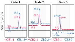 | 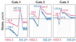 |
Vehicle 2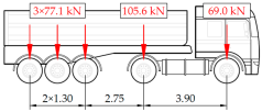 Type: 2—Total weight: 40.6 t | 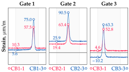 |  |
Vehicle 3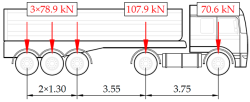 Type: 3—Total weight: 41.5 t | 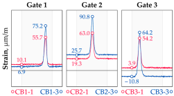 | 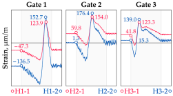 |
Vehicle 4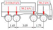 Type: 4—Total weight: 33.0 t | 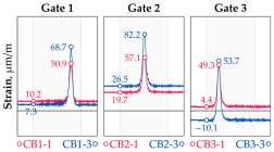 | 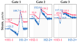 |
Vehicle 5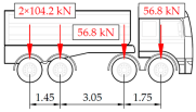 Type: 4—Total weight: 32.2 t | 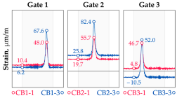 | 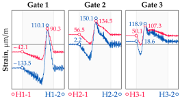 |
Vehicle 6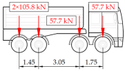 Type: 4—Total weight: 32.7 t | 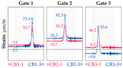 |  |
Vehicle 7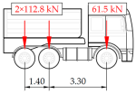 Type: 5—Total weight: 28.7 t | 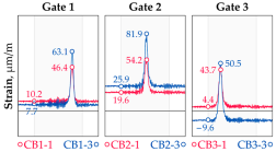 | 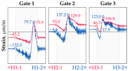 |
Vehicle 8 Type: 6—Total weight: 27.8 t |  |  |
Vehicle 9 Type: 7—Total weight: 28.8 t |  |  |
| Random Forest Regression: Total weight estimation number of trees: 500, max samples: 100.0% | |||
| Training Set Size | Training Time 1 [s] | RMSE [kg] | |
| Training Set | Test Set | ||
| 4800 | 5.5 | 518.1 | 1266.7 |
| 12,000 | 14.4 | 356.8 | 883.4 |
| 24,000 | 33.1 | 271.9 | 674.1 |
| 48,000 | 73.2 | 197.7 | 509.6 |
| Number of Inputs | Predictions | Linear Regression (LR) | Random Forest (RF) | Neural Network (NN) |
|---|---|---|---|---|
| 17 Inputs | Weight [kg] | 0.600 | 111.8 | 19.9 |
| Y Coordinate [m] | 1.016 | 0.038 | 0.017 | |
| 5 Inputs | Weight [kg] | 407.7 | 391.9 | 68.0 |
| Y Coordinate [m] | 1.015 | 0.069 | 0.013 | |
| 3 Inputs | Weight [kg] | 2323.1 | 1266.7 | 186.2 |
| Y Coordinate [m] | 1.096 | 0.127 | 0.036 |
Disclaimer/Publisher’s Note: The statements, opinions and data contained in all publications are solely those of the individual author(s) and contributor(s) and not of MDPI and/or the editor(s). MDPI and/or the editor(s) disclaim responsibility for any injury to people or property resulting from any ideas, methods, instructions or products referred to in the content. |
© 2025 by the authors. Licensee MDPI, Basel, Switzerland. This article is an open access article distributed under the terms and conditions of the Creative Commons Attribution (CC BY) license (https://creativecommons.org/licenses/by/4.0/).
Share and Cite
Piotrowski, D.; Jasiński, M.; Nowoświat, A.; Łaziński, P.; Pradelok, S. The Performance of an ML-Based Weigh-in-Motion System in the Context of a Network Arch Bridge Structural Specificity. Sensors 2025, 25, 4547. https://doi.org/10.3390/s25154547
Piotrowski D, Jasiński M, Nowoświat A, Łaziński P, Pradelok S. The Performance of an ML-Based Weigh-in-Motion System in the Context of a Network Arch Bridge Structural Specificity. Sensors. 2025; 25(15):4547. https://doi.org/10.3390/s25154547
Chicago/Turabian StylePiotrowski, Dawid, Marcin Jasiński, Artur Nowoświat, Piotr Łaziński, and Stefan Pradelok. 2025. "The Performance of an ML-Based Weigh-in-Motion System in the Context of a Network Arch Bridge Structural Specificity" Sensors 25, no. 15: 4547. https://doi.org/10.3390/s25154547
APA StylePiotrowski, D., Jasiński, M., Nowoświat, A., Łaziński, P., & Pradelok, S. (2025). The Performance of an ML-Based Weigh-in-Motion System in the Context of a Network Arch Bridge Structural Specificity. Sensors, 25(15), 4547. https://doi.org/10.3390/s25154547