
Source-Free Domain Adaptation Framework for Rotary Machine Fault Diagnosis


Abstract
1. Introduction
2. Related Work
2.1. Rotary Machine Fault Diagnosis
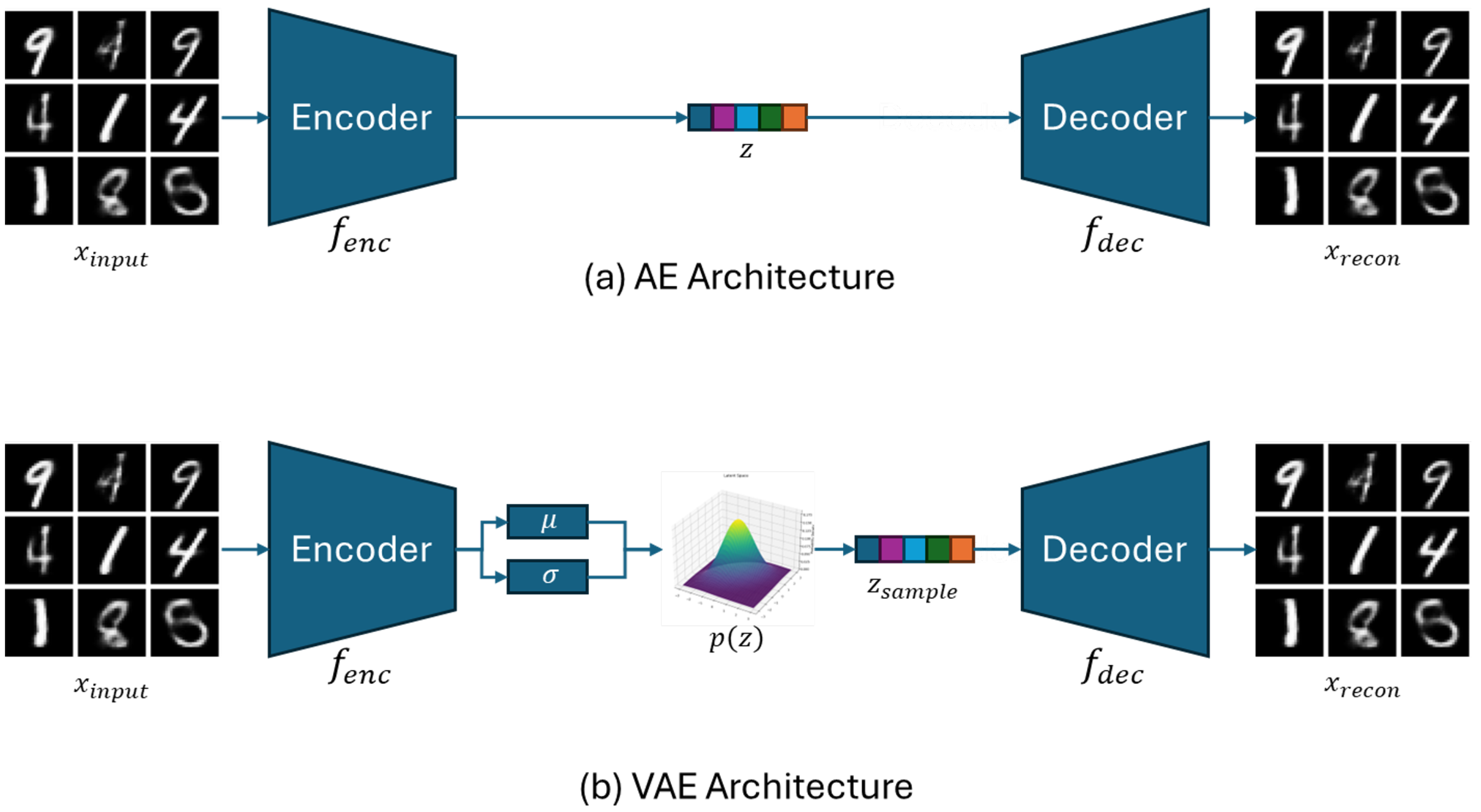
2.2. Self-Supervised Feature Extraction via VAE
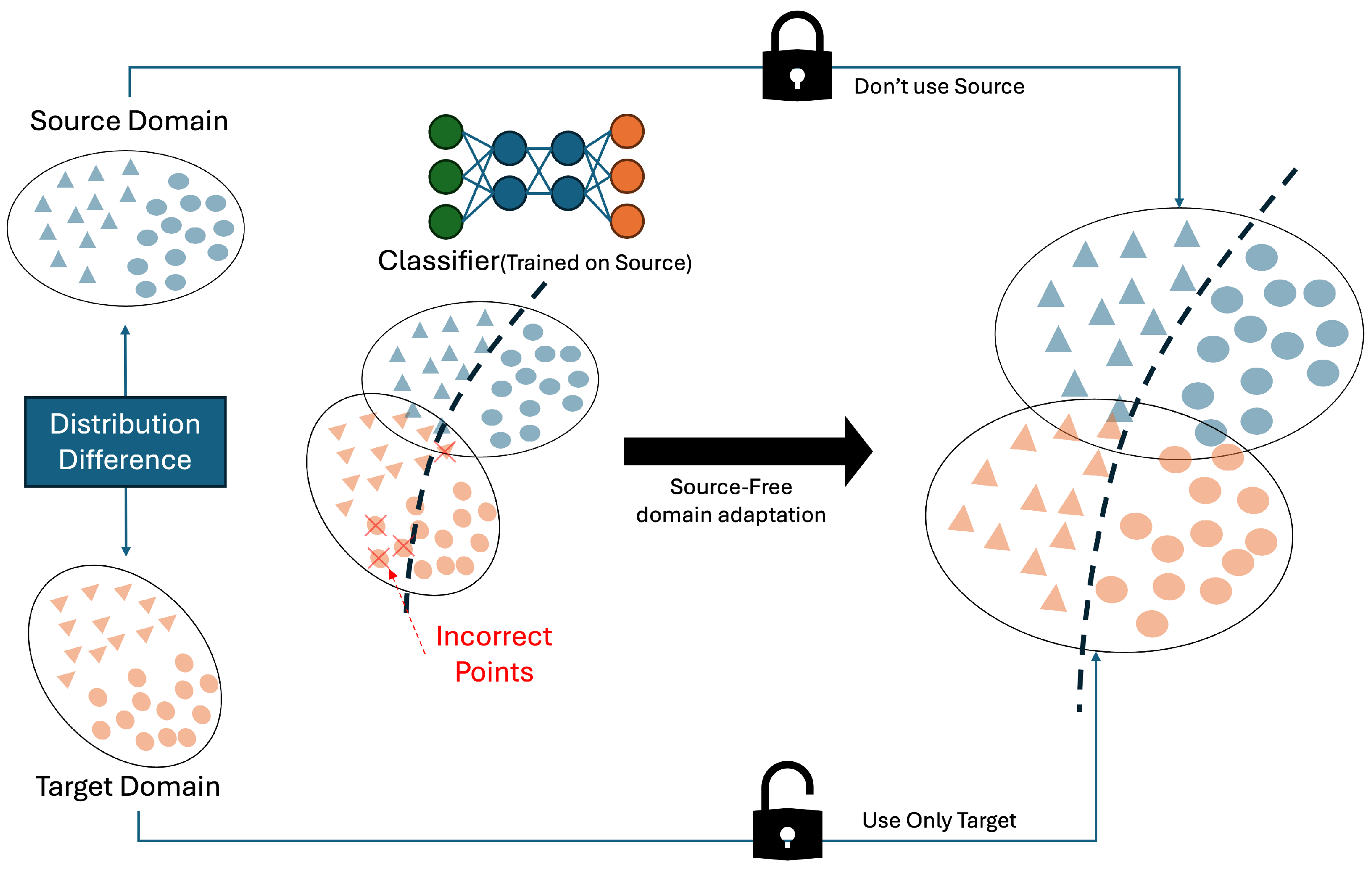
2.3. Source-Free Domain Adaptation
3. Method
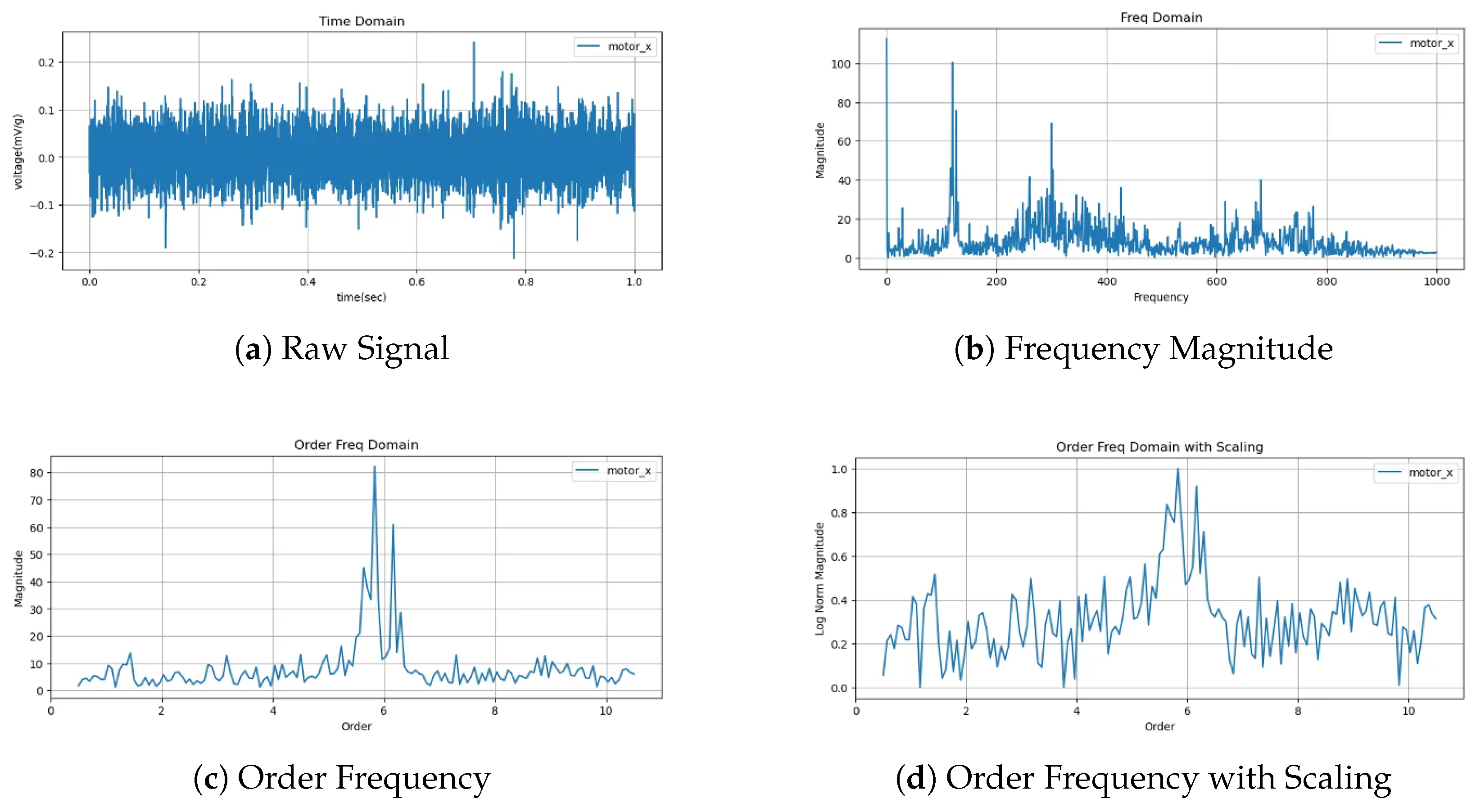
3.1. Mechanically Informed Order Spectrum Preprocessing
| Algorithm 1 Signal and reference preprocessing pipeline |
| Require: Input signal , Rotational speed , Machine ID m Ensure: Normalized order-domain pair:
|
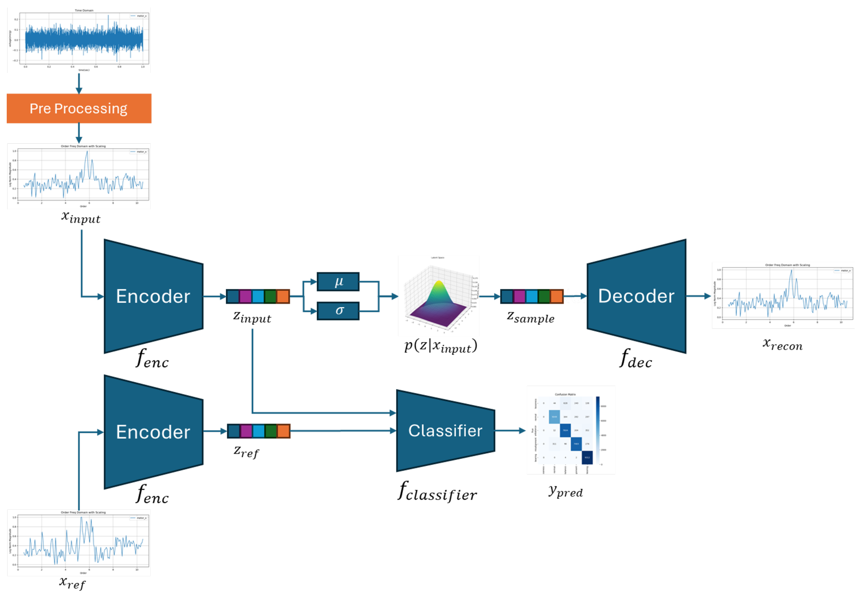
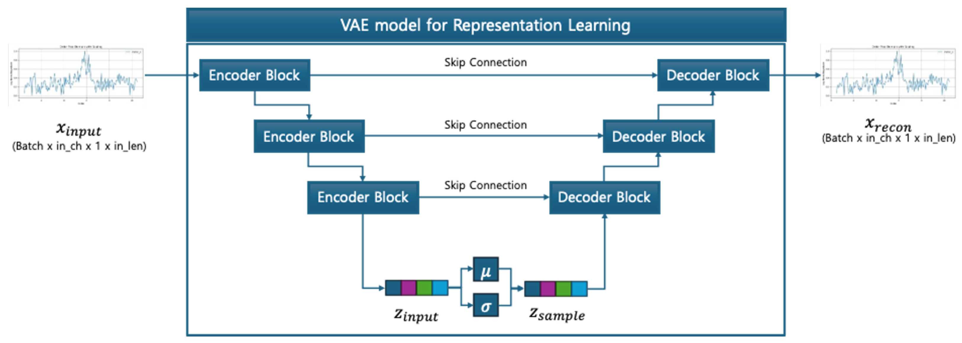
3.2. Latent Representation Learning via U-NetVAE with Difference-Aware Classification
3.3. Self-Supervised Test-Time Training for Domain Adaptation
3.3.1. Step 1: Self-Supervised Encoder Adaptation
- Reconstruction Loss: Loss between original input x and reconstruction :
- Augmentation Loss: Loss between reconstructed weak augmentation and original input x:
- Consistency Loss: Loss between reconstructed weak augmentation and reconstructed strong augmentation :
3.3.2. Step 2: Latent Fusion and Classification
4. Experiment
4.1. Dataset Integration
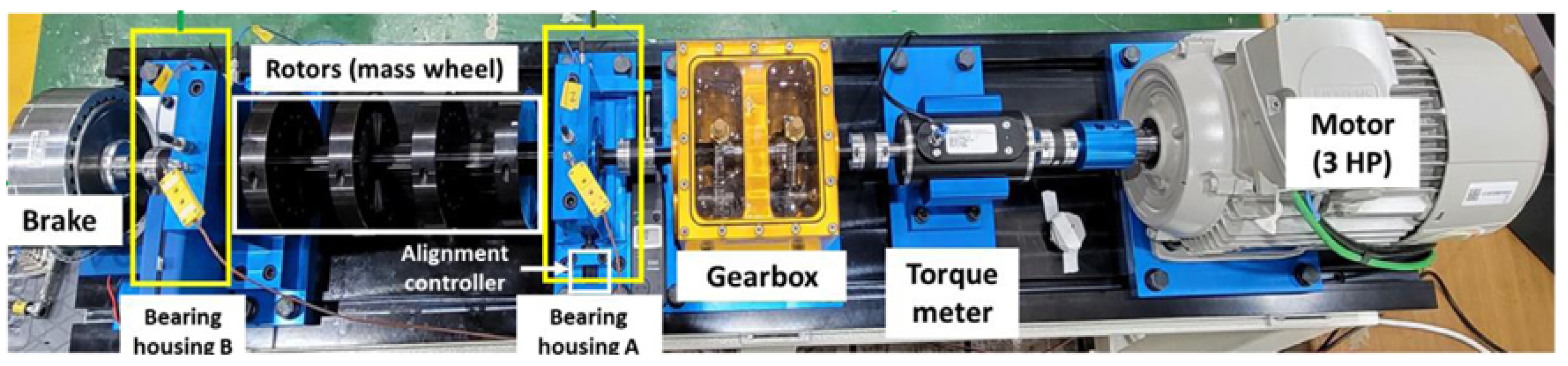
4.1.1. VAT
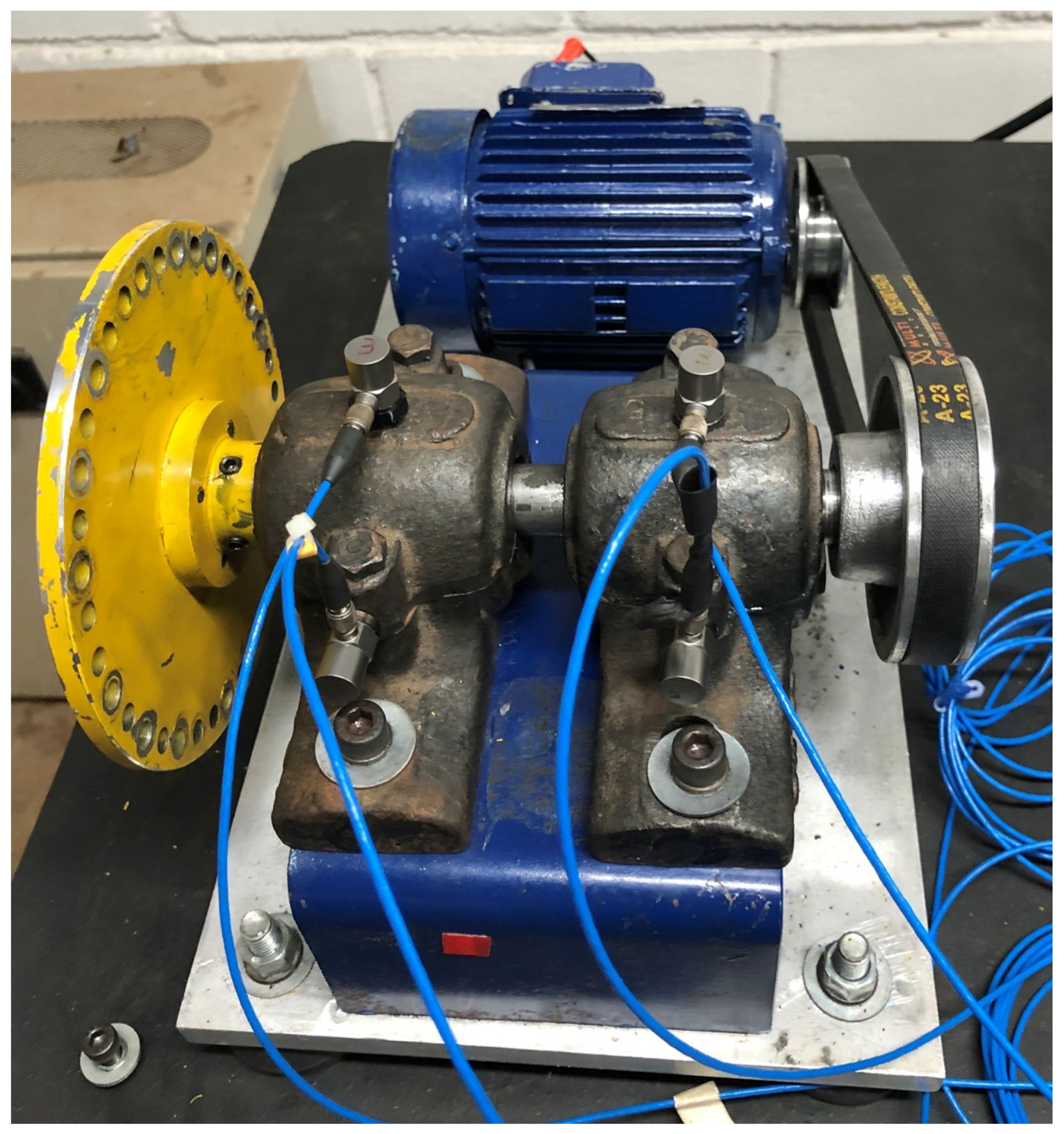
4.1.2. DXAI
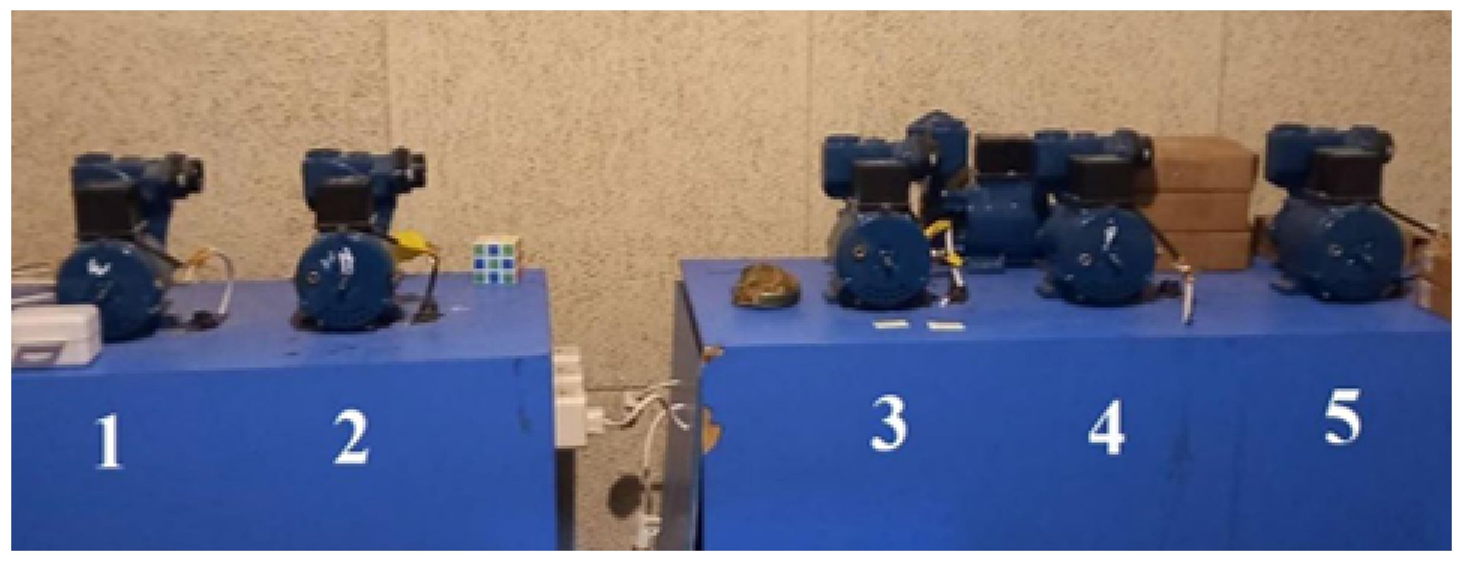
4.1.3. VBL-VA001
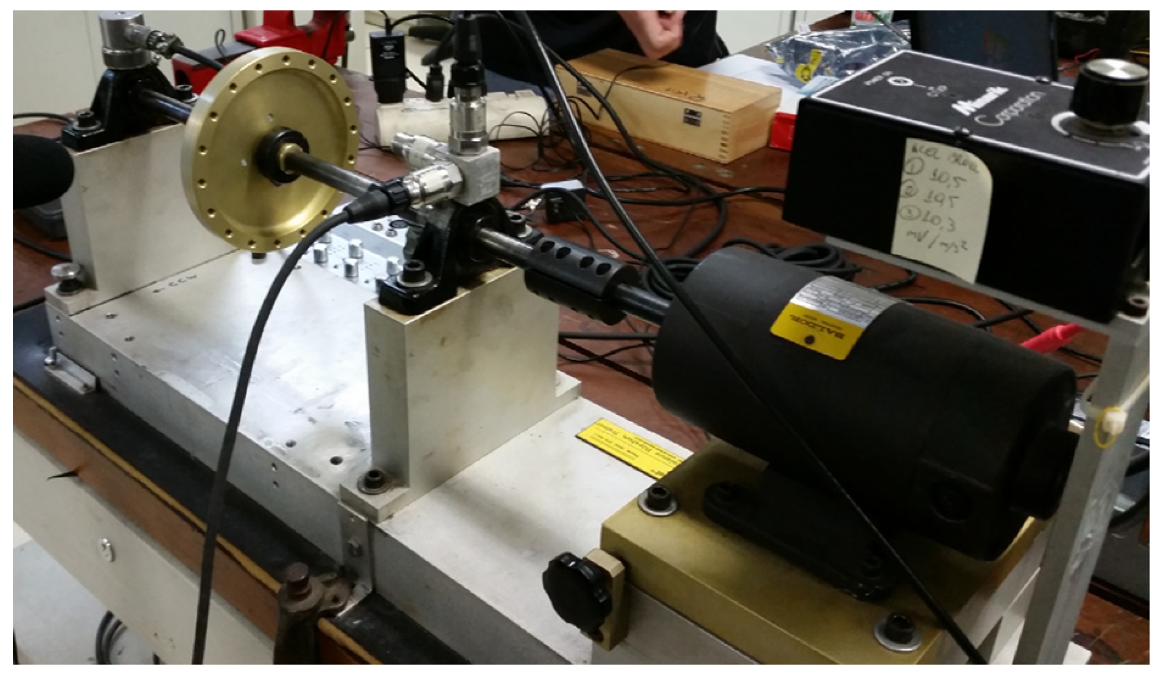
4.1.4. MaFaulDa
4.1.5. Integration Setting and Results
- Normal: healthy operating condition.
- Misalignment: shaft misalignment.
- Unbalance: rotor mass imbalance.
- Bearing: bearing-related faults (including outer race, inner race, and cage faults).
4.2. Benchmark
4.2.1. Benchmark Setting
- 1D-CNN: This is composed of three 1D convolutional blocks followed by a fully connected layer. Each block consists of a convolution layer, batch normalization, ReLU activation, and max pooling. The convolution layers use a kernel size of 3, a stride of 1, and padding of 1, with the output channels set to 16, 32, and 64, respectively.
- LSTM: This is constructed with two LSTM layers, each with a hidden dimension of 128. A dropout rate of 0.3 is applied between layers, and the input size is set to 2.
- Transformer: The embedding dimension is set to 64, and the number of heads in the multi-head attention is 4. The encoder output is summarized and passed through a fully connected layer to predict fault classes.
- Statistical features from the frequency domain: power, max frequency, mean frequency, median frequency, spectral skewness, spectral kurtosis, peak amplitude, band energy, dominant frequency power, spectral entropy, root-mean-square (RMS) frequency, frequency variance.
- Statistical features from the time domain: mean, standard deviation, max, min, RMS, skewness, kurtosis, peak, peak-to-peak value, crest factor, impulse factor, shape factor.
- Raw time-series signals.
- Frequency-domain signals generated through FFT transformation.
- Order-frequency-domain signals produced by the proposed preprocessing pipeline.
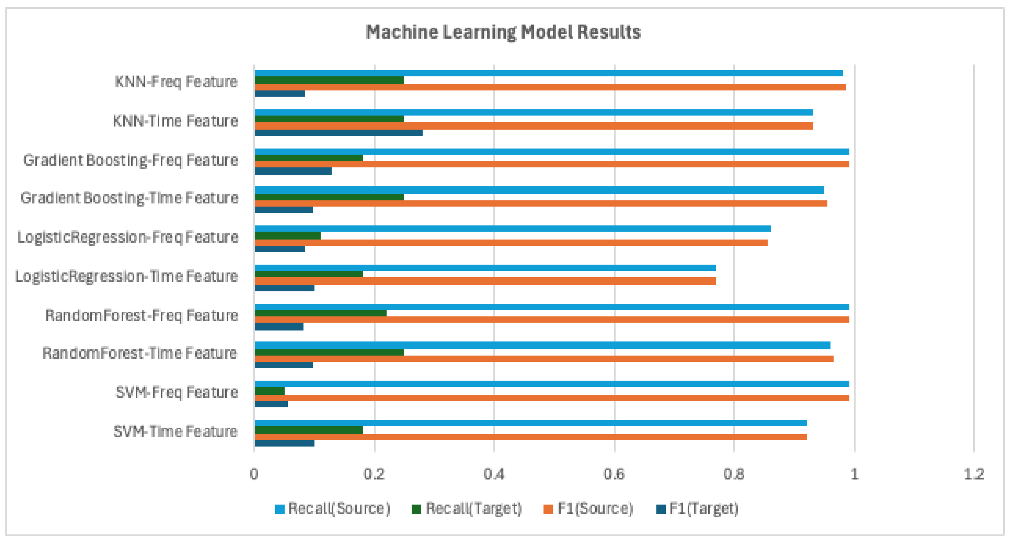
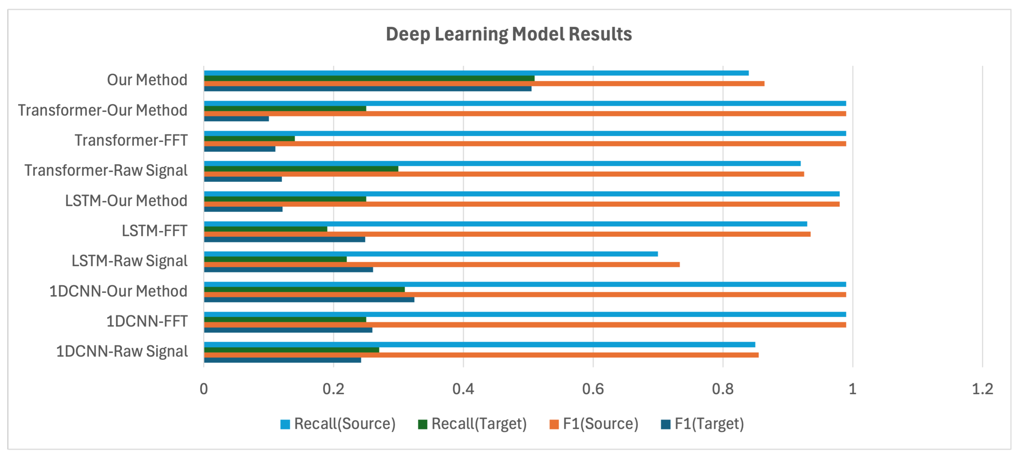
4.2.2. Benchmark Results
4.3. Model Implementation and Ablation Study
4.3.1. Model Implementation
4.3.2. Ablation Study
5. Conclusions
Author Contributions
Funding
Institutional Review Board Statement
Informed Consent Statement
Data Availability Statement
Conflicts of Interest
References
- Tang, B.; Liu, W.; Song, T. Wind turbine fault diagnosis based on Morlet wavelet transformation and Wigner-Ville distribution. Renew. Energy 2010, 35, 2862–2866. [Google Scholar] [CrossRef]
- Yan, R.; Gao, R.X.; Chen, X. Wavelets for fault diagnosis of rotary machines: A review with applications. Signal Process. 2014, 96, 1–15. [Google Scholar] [CrossRef]
- Konar, P.; Chattopadhyay, P. Bearing fault detection of induction motor using wavelet and Support Vector Machines (SVMs). Appl. Soft Comput. 2011, 11, 4203–4211. [Google Scholar] [CrossRef]
- Wan, X.; Wang, D.; Peter, W.T.; Xu, G.; Zhang, Q. A critical study of different dimensionality reduction methods for gear crack degradation assessment under different operating conditions. Measurement 2016, 78, 138–150. [Google Scholar] [CrossRef]
- Zhang, W.; Peng, G.; Li, C. Bearings fault diagnosis based on convolutional neural networks with 2-D representation of vibration signals as input. In MATEC Web of Conferences; EDP Sciences: Les Ulis, France, 2017; Volume 95, p. 13001. [Google Scholar]
- Ince, T.; Kiranyaz, S.; Eren, L.; Askar, M.; Gabbouj, M. Real-time motor fault detection by 1-D convolutional neural networks. IEEE Trans. Ind. Electron. 2016, 63, 7067–7075. [Google Scholar] [CrossRef]
- Guo, X.; Chen, L.; Shen, C. Hierarchical adaptive deep convolution neural network and its application to bearing fault diagnosis. Measurement 2016, 93, 490–502. [Google Scholar] [CrossRef]
- Ronneberger, O.; Fischer, P.; Brox, T. U-net: Convolutional networks for biomedical image segmentation. In Proceedings of the Medical Image Computing and Computer-Assisted Intervention–MICCAI 2015: 18th International Conference, Munich, Germany, 5–9 October 2015; Proceedings, Part III 18. Springer: Berlin/Heidelberg, Germany, 2015; pp. 234–241. [Google Scholar]
- Farrar, C.R.; Doebling, S.W.; Nix, D.A. Vibration–based structural damage identification. Philos. Trans. R. Soc. Lond. Ser. A Math. Phys. Eng. Sci. 2001, 359, 131–149. [Google Scholar] [CrossRef]
- Saha, D.K.; Hoque, M.E.; Badihi, H. Development of intelligent fault diagnosis technique of rotary machine element bearing: A machine learning approach. Sensors 2022, 22, 1073. [Google Scholar] [CrossRef]
- Lei, Y.; He, Z.; Zi, Y.; Hu, Q. Fault diagnosis of rotating machinery based on multiple ANFIS combination with GAs. Mech. Syst. Signal Process. 2007, 21, 2280–2294. [Google Scholar] [CrossRef]
- Zhang, W.; Li, C.; Peng, G.; Chen, Y.; Zhang, Z. A deep convolutional neural network with new training methods for bearing fault diagnosis under noisy environment and different working load. Mech. Syst. Signal Process. 2018, 100, 439–453. [Google Scholar] [CrossRef]
- Shao, J.; Huang, Z.; Zhu, Y.; Zhu, J.; Fang, D. Rotating machinery fault diagnosis by deep adversarial transfer learning based on subdomain adaptation. Adv. Mech. Eng. 2021, 13, 16878140211040226. [Google Scholar] [CrossRef]
- Aiordăchioaie, D. A comparative analysis of fault detection and process diagnosis methods based on a signal processing paradigm. Discov. Appl. Sci. 2025, 7, 10. [Google Scholar] [CrossRef]
- Wang, T.; Li, J.; Zhang, P.; Sun, Y. Fault diagnosis of rotating machinery under time-varying speed based on order tracking and deep learning. J. Vibroeng. 2020, 22, 366–382. [Google Scholar] [CrossRef]
- Yu, X.; Feng, Z.; Zhang, D. Adaptive high-resolution order spectrum for complex signal analysis of rotating machinery: Principle and applications. Mech. Syst. Signal Process. 2022, 177, 109194. [Google Scholar] [CrossRef]
- He, K.; Chen, X.; Xie, S.; Li, Y.; Dollár, P.; Girshick, R. Masked autoencoders are scalable vision learners. In Proceedings of the IEEE/CVF Conference on Computer Vision and Pattern Recognition, New Orleans, LA, USA, 21–24 June 2022; pp. 16000–16009. [Google Scholar]
- Maaløe, L.; Sønderby, C.K.; Sønderby, S.K.; Winther, O. Auxiliary deep generative models. In Proceedings of the International Conference on Machine Learning, PMLR, New York, NY, USA, 20–22 June 2016; pp. 1445–1453. [Google Scholar]
- Ding, Z.; Xu, Y.; Xu, W.; Parmar, G.; Yang, Y.; Welling, M.; Tu, Z. Guided variational autoencoder for disentanglement learning. In Proceedings of the IEEE/CVF Conference on Computer Vision and Pattern Recognition, Seattle, WA, USA, 13–19 June 2020; pp. 7920–7929. [Google Scholar]
- Kingma, D.P.; Welling, M. Auto-encoding variational bayes. arXiv 2013, arXiv:1312.6114v10. [Google Scholar]
- Bengio, Y.; Courville, A.; Vincent, P. Representation learning: A review and new perspectives. IEEE Trans. Pattern Anal. Mach. Intell. 2013, 35, 1798–1828. [Google Scholar] [CrossRef]
- Li, J.; Ren, W.; Han, M. Mutual information variational autoencoders and its application to feature extraction of multivariate time series. Int. J. Pattern Recognit. Artif. Intell. 2022, 36, 2255005. [Google Scholar] [CrossRef]
- Erhan, D.; Courville, A.; Bengio, Y.; Vincent, P. Why does unsupervised pre-training help deep learning? In Proceedings of the Thirteenth International Conference on Artificial Intelligence and Statistics, Sardinia, Italy, 13–15 May 2010; JMLR Workshop and Conference Proceedings. pp. 201–208. [Google Scholar]
- Gouda, W.; Tahir, S.; Alanazi, S.; Almufareh, M.; Alwakid, G. Unsupervised outlier detection in IOT using deep VAE. Sensors 2022, 22, 6617. [Google Scholar] [CrossRef]
- Huang, T.; Chen, P.; Li, R. A semi-supervised VAE based active anomaly detection framework in multivariate time series for online systems. In Proceedings of the ACM Web Conference 2022, Lyon, France, 25–29 April 2022; pp. 1797–1806. [Google Scholar]
- Higgins, I.; Matthey, L.; Pal, A.; Burgess, C.; Glorot, X.; Botvinick, M.; Mohamed, S.; Lerchner, A. beta-vae: Learning basic visual concepts with a constrained variational framework. In Proceedings of the International Conference on Learning Representations, Toulon, France, 24–26 April 2017. [Google Scholar]
- Liang, J.; Hu, D.; Feng, J. Do we really need to access the source data? Source hypothesis transfer for unsupervised domain adaptation. In Proceedings of the International Conference on Machine Learning, PMLR, Virtual, 13–18 July 2020; pp. 6028–6039. [Google Scholar]
- Sun, Y.; Wang, X.; Liu, Z.; Miller, J.; Efros, A.; Hardt, M. Test-time training with self-supervision for generalization under distribution shifts. In Proceedings of the International Conference on Machine Learning, PMLR, Virtual, 13–18 July 2020; pp. 9229–9248. [Google Scholar]
- Chen, D.; Wang, D.; Darrell, T.; Ebrahimi, S. Contrastive test-time adaptation. In Proceedings of the IEEE/CVF Conference on Computer Vision and Pattern Recognition, New Orleans, LA, USA, 21–24 June 2022; pp. 295–305. [Google Scholar]
- Darestani, M.Z.; Liu, J.; Heckel, R. Test-time training can close the natural distribution shift performance gap in deep learning based compressed sensing. In Proceedings of the International Conference on Machine Learning, PMLR, Baltimore, MD, USA, 17–23 July 2022; pp. 4754–4776. [Google Scholar]
- Sinha, S.; Gehler, P.; Locatello, F.; Schiele, B. Test: Test-time self-training under distribution shift. In Proceedings of the IEEE/CVF Winter Conference on Applications of Computer Vision, Waikoloa, HI, USA, 2–7 January 2023; pp. 2759–2769. [Google Scholar]
- Wang, Y.; Gong, P.; Wu, M.; Ott, F.; Li, X.; Xie, L.; Chen, Z. Temporal Source Recovery for Time-Series Source-Free Unsupervised Domain Adaptation. arXiv 2024, arXiv:2409.19635. [Google Scholar]
- Ragab, M.; Eldele, E.; Wu, M.; Foo, C.S.; Li, X.; Chen, Z. Source-free domain adaptation with temporal imputation for time series data. In Proceedings of the 29th ACM SIGKDD Conference on Knowledge Discovery and Data Mining, Long Beach, CA, USA, 6–10 August 2023; pp. 1989–1998. [Google Scholar]
- Mohammadi, S.; Belgiu, M.; Stein, A. A source-free unsupervised domain adaptation method for cross-regional and cross-time crop mapping from satellite image time series. Remote Sens. Environ. 2024, 314, 114385. [Google Scholar] [CrossRef]
- Leturiondo, U.; Mishra, M.; Galar, D.; Salgado, O. Synthetic data generation in hybrid modelling of rolling element bearings. Insight-Non-Destr. Test. Cond. Monit. 2015, 57, 395–400. [Google Scholar] [CrossRef]
- Sobie, C.; Freitas, C.; Nicolai, M. Simulation-driven machine learning: Bearing fault classification. Mech. Syst. Signal Process. 2018, 99, 403–419. [Google Scholar] [CrossRef]
- Matania, O.; Cohen, R.; Bechhoefer, E.; Bortman, J. Zero-fault-shot learning for bearing spall type classification by hybrid approach. Mech. Syst. Signal Process. 2025, 224, 112117. [Google Scholar] [CrossRef]
- Cooley, J.W.; Tukey, J.W. An algorithm for the machine calculation of complex Fourier series. Math. Comput. 1965, 19, 297–301. [Google Scholar] [CrossRef]
- Gabor, D. Theory of communication. Part 1: The analysis of information. J. Inst. Electr. Eng.-Part III Radio Commun. Eng. 1946, 93, 429–441. [Google Scholar] [CrossRef]
- Mallat, S. A Wavelet Tour of Signal Processing; Elsevier: Amsterdam, The Netherlands, 1999. [Google Scholar]
- Xue, H.; Wang, H.; Song, L.; Chen, P. Structural fault diagnosis of rotating machinery based on distinctive frequency components and support vector machines. In Proceedings of the International Conference on Intelligent Computing, Chongqing, China, 8–9 January 2011; Springer: Berlin/Heidelberg, Germany, 2011; pp. 341–348. [Google Scholar]
- Wu, J.D.; Bai, M.R.; Su, F.C.; Huang, C.W. An expert system for the diagnosis of faults in rotating machinery using adaptive order-tracking algorithm. Expert Syst. Appl. 2009, 36, 5424–5431. [Google Scholar] [CrossRef]
- Bai, M.R.; Jeng, J.; Chen, C. Adaptive order tracking technique using recursive least-square algorithm. J. Vib. Acoust. 2002, 124, 502–511. [Google Scholar] [CrossRef]
- Jung, W.; Kim, S.H.; Yun, S.H.; Bae, J.; Park, Y.H. Vibration, acoustic, temperature, and motor current dataset of rotating machine under varying operating conditions for fault diagnosis. Data Brief 2023, 48, 109049. [Google Scholar] [CrossRef] [PubMed]
- Atmaja, B.T.; Ihsannur, H.; Suyanto; Arifianto, D. Lab-scale vibration analysis dataset and baseline methods for machinery fault diagnosis with machine learning. J. Vib. Eng. Technol. 2024, 12, 1991–2001. [Google Scholar] [CrossRef]
- Marins, M.A.; Ribeiro, F.M.; Netto, S.L.; Da Silva, E.A. Improved similarity-based modeling for the classification of rotating-machine failures. J. Frankl. Inst. 2018, 355, 1913–1930. [Google Scholar] [CrossRef]
- Brito, L.C.; Susto, G.A.; Brito, J.N.; Duarte, M.A. Mechanical Faults in Rotating Machinery Dataset (Normal, Unbalance, Misalignment, Looseness). 2022. Available online: https://www.research.unipd.it/handle/11577/3469613 (accessed on 17 April 2025).
- Cortes, C.; Vapnik, V. Support-vector networks. Mach. Learn. 1995, 20, 273–297. [Google Scholar] [CrossRef]
- Hosmer, D.W., Jr.; Lemeshow, S.; Sturdivant, R.X. Applied Logistic Regression; John Wiley & Sons: Hoboken, NJ, USA, 2013. [Google Scholar]
- Breiman, L. Random forests. Mach. Learn. 2001, 45, 5–32. [Google Scholar] [CrossRef]
- Friedman, J.H. Greedy function approximation: A gradient boosting machine. Ann. Stat. 2001, 29, 1189–1232. [Google Scholar] [CrossRef]
- Cover, T.; Hart, P. Nearest neighbor pattern classification. IEEE Trans. Inf. Theory 1967, 13, 21–27. [Google Scholar] [CrossRef]
- LeCun, Y.; Boser, B.; Denker, J.S.; Henderson, D.; Howard, R.E.; Hubbard, W.; Jackel, L.D. Backpropagation applied to handwritten zip code recognition. Neural Comput. 1989, 1, 541–551. [Google Scholar] [CrossRef]
- Hochreiter, S.; Schmidhuber, J. Long short-term memory. Neural Comput. 1997, 9, 1735–1780. [Google Scholar] [CrossRef] [PubMed]
- Ashish, V. Attention is all you need. Adv. Neural Inf. Process. Syst. 2017, 30, I. [Google Scholar]
- Liu, Y.; Kothari, P.; Van Delft, B.; Bellot-Gurlet, B.; Mordan, T.; Alahi, A. Ttt++: When does self-supervised test-time training fail or thrive? Adv. Neural Inf. Process. Syst. 2021, 34, 21808–21820. [Google Scholar]
- Iwasawa, Y.; Matsuo, Y. Test-time classifier adjustment module for model-agnostic domain generalization. Adv. Neural Inf. Process. Syst. 2021, 34, 2427–2440. [Google Scholar]
- Jang, M.; Chung, S.Y.; Chung, H.W. Test-time adaptation via self-training with nearest neighbor information. arXiv 2022, arXiv:2207.10792. [Google Scholar]
- Jang, G.D.; Han, D.K.; Lee, S.W. Test-Time Adaptation for EEG-Based Driver Drowsiness Classification. In Proceedings of the International Conference on Pattern Recognition and Artificial Intelligence, Xiamen, China, 20–22 September 2024; Springer: Berlin/Heidelberg, Germany, 2024; pp. 410–424. [Google Scholar]
- Ragab, M.; Eldele, E.; Tan, W.L.; Foo, C.S.; Chen, Z.; Wu, M.; Kwoh, C.K.; Li, X. Adatime: A benchmarking suite for domain adaptation on time series data. ACM Trans. Knowl. Discov. Data 2023, 17, 1–18. [Google Scholar] [CrossRef]


| Datasets | VAT | VBL-VA001 | |
|---|---|---|---|
| Items | |||
| Motor | Four-pole AC motor by SIEMENS, Germany (3HP) | Panasonic, Japan GP-129JXK (125W, 3000RPM) | |
| Accelerometers | 4× PCB352C34 at bearings A, B, United States | LOG-0002-100G on motor (X,Y,Z), United States | |
| Other Sensors | Acoustic mic, 4× CT sensor, 2× K-type thermocouples | - | |
| Sampling Frequency | 25.6 kHz (vibration/temp), 51.2 kHz (acoustic) | 20 kHz | |
| Fault Types | Bearing fault, unbalance, misalignment | Normal, misalignment, unbalance (2 levels), BPFO | |
| Operating Conditions | Load: 0, 2, 4 Nm/RPM: 3010, 680–2460 | Fixed 3000 RPM | |
| Acquisition Time and Repetition | Normal: 120s, Faulty: 60 s, 7 × 300 s, 1 × 600 s | 1000 samples/class, 5 s/sample | |
| Data Collection Institution | Korea Advanced Institute of Science and Technology | Sepuluh Nopember Institute of Technology, Indonesia | |
| Source | Jung et al. (2023) [44], Mendeley Data, 10.17632/vxkj334rzv.7 | Atmaja et al. (2024) [45], J. Vibration Eng. Tech. 12(2) | |
| MaFaulDA | DXAI | |
|---|---|---|
| Motor | DC motor, 1/4CV, ABVT trainer, United States | Three-phase induction motor, B56 B4, 1650 RPM, 0.09 kW, 220 V, 0.70 A, Germany |
| Accelerometers | IMI 601A01, IMI 604B31, United States | 4× PCB352C33 (2 per bearing), United States |
| Other Sensors | Shure(United States) SM81 condenser microphone | - |
| Sampling Frequency | 50 kHz | 25 kHz |
| Fault Types | 8568 labeled faults | Normal, unbalance, misalignment, looseness |
| Operating Conditions | 60–3686 RPM (varied) | Fixed 1238 RPM |
| Acquisition Time and Repetition | 1951 samples (varied), 5 s/sample | 5 tests/class, 420 samples/test, 1 s/sample |
| Data Collection Institution | Federal University of Rio de Janeiro | Univ. of São João del-Rei, Universidade Federal de Uberlandia, Universita degli Studi di Padova |
| Source | MaFaulDa Database (2018) [46], www02.smt.ufrj.br/~offshore/mfs, accessed on 17 April 2025 | Lucas Brito et al. (2022) [47], Expert Systems with Applications, 10.1016/j.eswa.2023.120860 |
| Dataset | VAT-MCD | VBL-VA001 | MaFaulDA | DXAI | Total | |
|---|---|---|---|---|---|---|
| Class | ||||||
| normal | 1077 | 8000 | 392 | 2100 | 11,569 | |
| misalignment | 2151 | 8000 | 3984 | 2100 | 16,235 | |
| unbalance | 3585 | 8000 | 2664 | 2100 | 16,349 | |
| bearing | 2142 | 8000 | 8568 | - | 18,710 | |
| Total | 8955 | 32,000 | 15,608 | 7145 | 62,863 | |
| Model Name | Data Preprocessing Method | Validation (Source Domain) | Test (Target Domain) |
|---|---|---|---|
| SVM | Time Feature | precision: 0.92; recall: 0.92; F1: 0.92 | precision: 0.07; recall: 0.18; F1: 0.09 |
| Frequency Feature | precision: 0.99; recall: 0.99; F1: 0.99 | precision: 0.06; recall: 0.05; F1: 0.05 | |
| Random Forest | Time Feature | precision: 0.97; recall: 0.96; F1: 0.97 | precision: 0.06; recall: 0.25; F1: 0.10 |
| Frequency Feature | precision: 0.99; recall: 0.99; F1: 0.99 | precision: 0.05; recall: 0.22; F1: 0.08 | |
| Logistic Regression | Time Feature | precision: 0.77; recall: 0.77; F1: 0.76 | precision: 0.07; recall: 0.18; F1: 0.10 |
| Frequency Feature | precision: 0.85 recall: 0.86;; F1: 0.85 | precision: 0.07; recall: 0.11; F1: 0.08 | |
| Gradient Boosting | Time Feature | precision: 0.96; recall: 0.95; F1: 0.96 | precision: 0.06; recall: 0.25; F1: 0.10 |
| Frequency Feature | precision: 0.99; recall: 0.99; F1: 0.99 | precision: 0.10; recall: 0.18; F1: 0.12 | |
| KNN | Time Feature | precision: 0.93; recall: 0.93; F1: 0.93 | precision: 0.32; recall: 0.25; F1: 0.28 |
| Frequency Feature | precision: 0.99; recall: 0.98; F1: 0.99 | precision: 0.05; recall: 0.25; F1: 0.08 | |
| 1D-CNN | Raw Signal | precision: 0.86; recall: 0.85; F1: 0.85 | precision: 0.22; recall: 0.27; F1: 0.24 |
| FFT | precision: 0.99; recall: 0.99; F1: 0.99 | precision: 0.27; recall: 0.25; F1: 0.25 | |
| Our Method | precision: 0.99; recall: 0.99; F1: 0.99 | precision: 0.34; recall: 0.31; F1: 0.32 | |
| Raw Signal | precision: 0.77; recall: 0.70; F1: 0.69 | precision: 0.32; recall: 0.22; F1: 0.26 | |
| LSTM | FFT | precision: 0.94; recall: 0.93; F1: 0.93 | precision: 0.36; recall: 0.19; F1: 0.24 |
| Our Method | precision: 0.98; recall: 0.98; F1: 0.98 | precision: 0.08; recall: 0.25; F1: 0.12 | |
| Raw Signal | precision: 0.93; recall: 0.92; F1: 0.92 | precision: 0.40; recall: 0.30; F1: 0.21 | |
| Transformer | FFT | precision: 0.99; recall: 0.99; F1: 0.99 | precision: 0.34; recall: 0.14; F1: 0.11 |
| Our Method | precision: 0.99; recall: 0.99; F1: 0.99 | precision: 0.57; recall: 0.25; F1: 0.10 | |
| Our Method | Our Method | precision: 0.89; recall: 0.84; F1: 0.86 | precision: 0.50; recall: 0.51; F1: 0.50 |
| Model | Scheduler | Optimizer (Training) | Optimizer (TTT) |
|---|---|---|---|
| U-NetVAE | StepLR | Adam | SGD (Only Encoder) |
| Classifier | Cosine Annealing | Adam | - |
| Experiment Setting | Order Preprocessing | Reconstruction | TTT | Source Domain Test | Target Domain Test |
|---|---|---|---|---|---|
| Baseline | x | x | x | precision: 0.89 recall: 0.83 F1: 0.82 | precision: 0.26 recall: 0.26 F1: 0.23 |
| +Order Spectrum Preprocessing | o | x | x | precision: 0.89 recall: 0.84 F1: 0.84 | precision: 0.48 recall: 0.50 F1: 0.46 |
| +Reconstruction | o | o | x | precision: 0.89 recall: 0.84 F1: 0.84 | precision: 0.48 recall: 0.50 F1: 0.46 |
| +Ours | o | o | o | precision: 0.89 recall: 0.84 F1: 0.86 | precision: 0.50 recall: 0.51 F1: 0.50 |
| Model | Precision (Source) | Recall (Source) | F1 (Source) | Precision (Target) | Recall (Target) | F1 (Target) |
|---|---|---|---|---|---|---|
| VAE | 0.86 | 0.74 | 0.80 | 0.15 | 0.16 | 0.15 |
| VQ-VAE | 0.81 | 0.78 | 0.79 | 0.38 | 0.32 | 0.35 |
| U-Net-VAE (Ours) | 0.89 | 0.84 | 0.86 | 0.50 | 0.51 | 0.50 |
| Model | Precision (Target) | Recall (Target) | F1 (Target) |
|---|---|---|---|
| T3A | 0.28 | 0.33 | 0.30 |
| TAST | 0.43 | 0.31 | 0.36 |
| U-Net-VAE (Ours) | 0.50 | 0.51 | 0.50 |
Disclaimer/Publisher’s Note: The statements, opinions and data contained in all publications are solely those of the individual author(s) and contributor(s) and not of MDPI and/or the editor(s). MDPI and/or the editor(s) disclaim responsibility for any injury to people or property resulting from any ideas, methods, instructions or products referred to in the content. |
© 2025 by the authors. Licensee MDPI, Basel, Switzerland. This article is an open access article distributed under the terms and conditions of the Creative Commons Attribution (CC BY) license (https://creativecommons.org/licenses/by/4.0/).
Share and Cite
Jeong, H.; Kim, S.; Seo, D.; Kwon, J. Source-Free Domain Adaptation Framework for Rotary Machine Fault Diagnosis. Sensors 2025, 25, 4383. https://doi.org/10.3390/s25144383
Jeong H, Kim S, Seo D, Kwon J. Source-Free Domain Adaptation Framework for Rotary Machine Fault Diagnosis. Sensors. 2025; 25(14):4383. https://doi.org/10.3390/s25144383
Chicago/Turabian StyleJeong, Hoejun, Seungha Kim, Donghyun Seo, and Jangwoo Kwon. 2025. "Source-Free Domain Adaptation Framework for Rotary Machine Fault Diagnosis" Sensors 25, no. 14: 4383. https://doi.org/10.3390/s25144383
APA StyleJeong, H., Kim, S., Seo, D., & Kwon, J. (2025). Source-Free Domain Adaptation Framework for Rotary Machine Fault Diagnosis. Sensors, 25(14), 4383. https://doi.org/10.3390/s25144383