
Coverage Hole Recovery in Hybrid Sensor Networks Based on Key Perceptual Intersections for Emergency Communications

 , ,
, ,  and
and
Abstract

1. Introduction
2. Related Work
2.1. Static Sensor Networks
2.2. Mobile Sensor Networks
2.3. Hybrid Sensor Networks
3. System Model
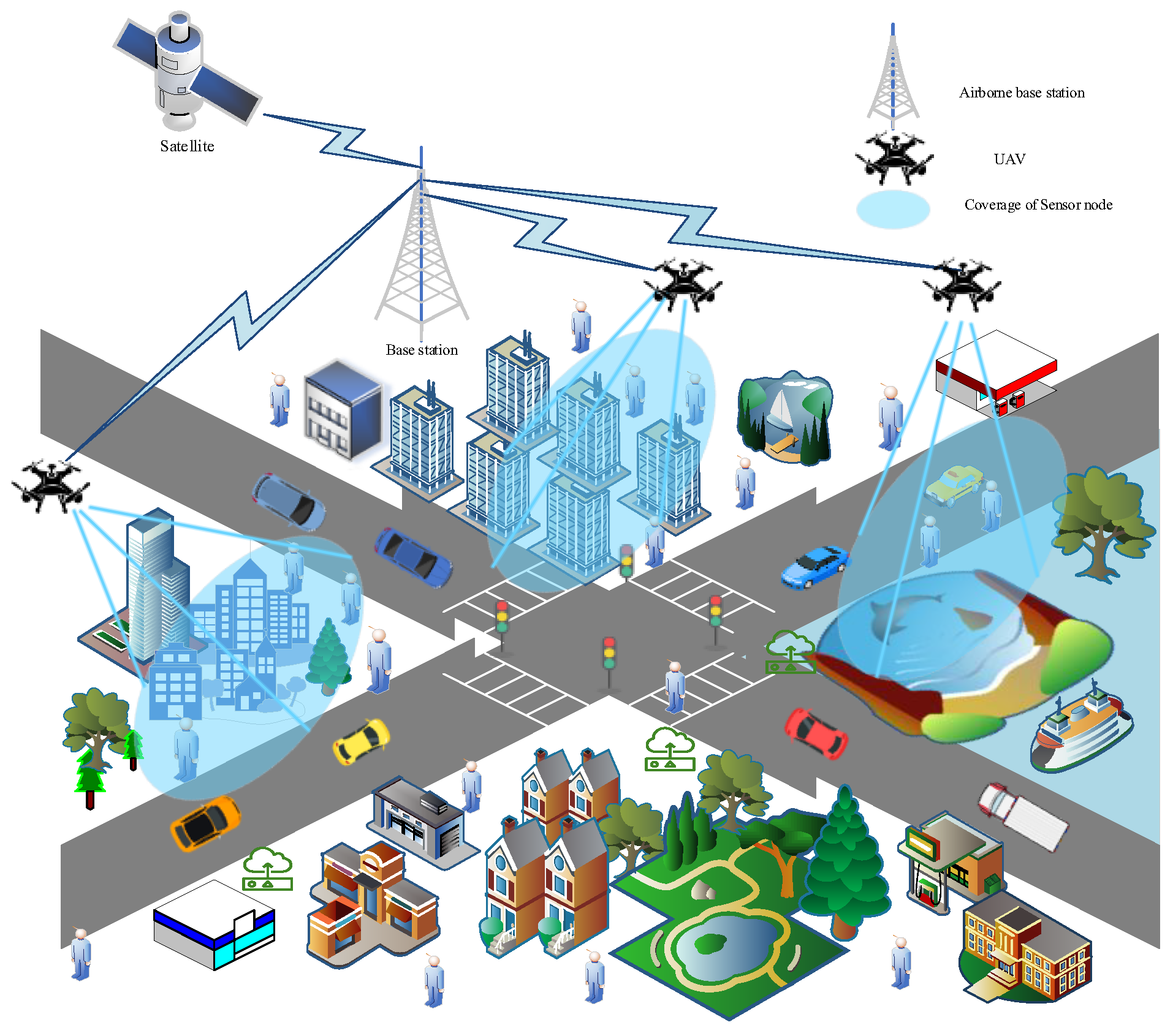
3.1. Network Model
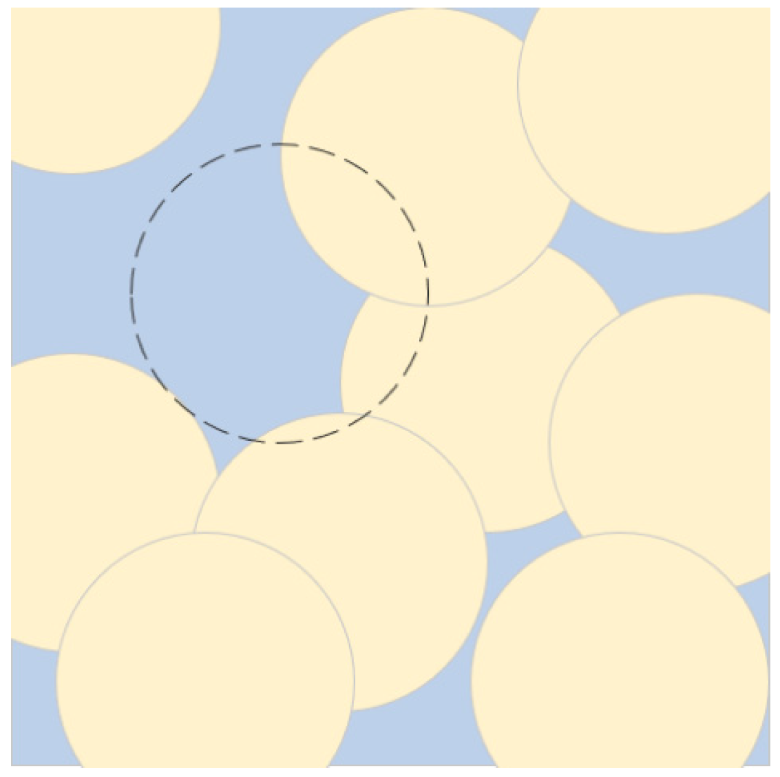
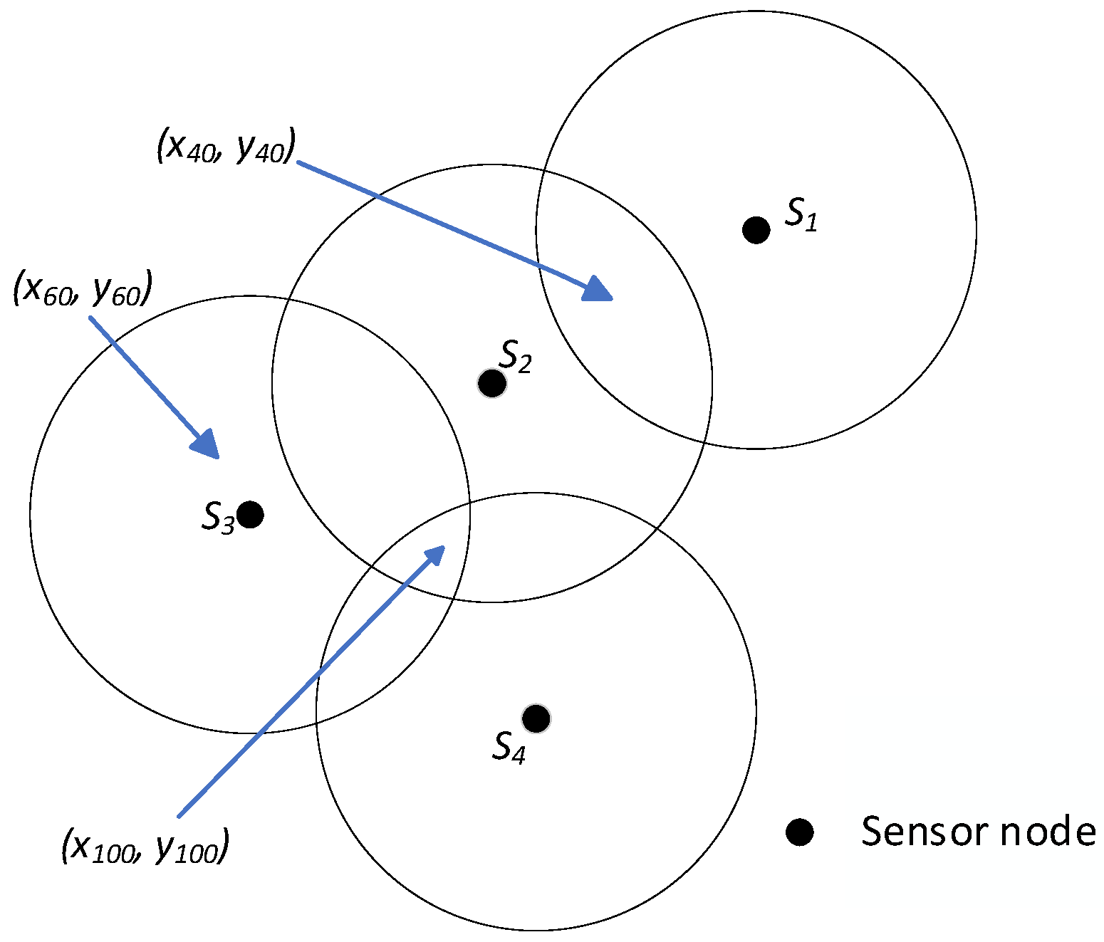
3.2. Sensing Model
3.3. Energy Model
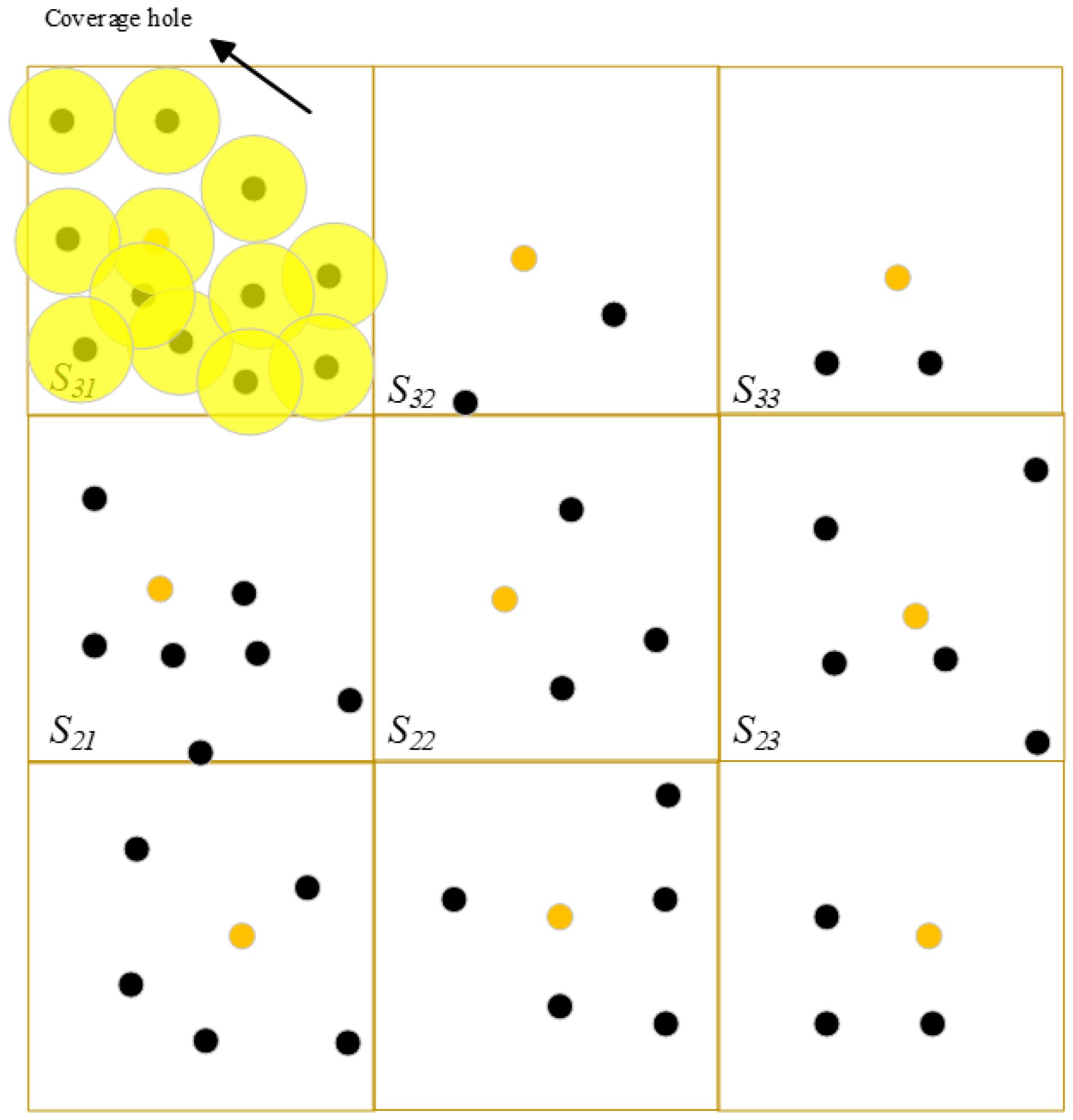
3.4. Hole Model
3.5. Network Scenario
4. Proposed Methodology
4.1. Network Unit
| Algorithm 1. Network unit |
| Input: i: row number, j: column number, L: length of the network, C: number of network units, n: number of nodes |
| Output: C, Aij 1: The network density is calculated 2: Density = n/L2 3: The number of units is calculated according to the Density 4: Each unit is named as Aij 5: The side size of each unit in the network is calculated by 6: The base station notifies (x0, y0) and Cellsize to all network nodes 7: for (s = 1; s ≤ n; s++) do 8: Identifying unit number in which it is located for nodes by 9: Node s sends a hello packet to the neighbor nodes 10: end for 11: if (The node has the most remaining energy and closest to the center of the unit) then 12: Sends a packet and declares itself a unit agent 13: else 14: Waits to receive the unit agent notification packet 15: end if |
4.2. Detecting Holes
| Algorithm 2. Detecting Holes |
| Input: k: number of pixels covered by the unit, n: number of nodes, d: Euclidean distance, C: number of network units, Rs: sensing radius |
| Output: Coverageratesij 1: Information = 0 2: for (s = 1; s ≤ C; s++) do 3: for (k = 1; d ≤ Rs; k++) do 4: All the entries of a row k in the Info table are OR together and recorded in CoNO column 5: end for 6: Calculate the coverage of each unit (Coverageratesij) 7: end for 8: for (s = 1; s ≤ C; s++) do 9: if (Coverageratesij < 90%) then 10: This unit has holes. 11: else 12: There are no holes in this unit. 13: end if |
4.3. Hole Recovery
| Algorithm 3. Hole Recovery |
| Input: z: number of coverage hole, m: number of mobile nodes, n: the number of key perceptual point |
| Output: New coverage of Unit Sij 1: Coverageratesij < 90% 2: if z ≤ m then 3: for (z = 1; z ≤ m; z++) do 4: The mobile node is directly sent to the coordinates for hole recovery by . 5: else 6: for (z = 1; z > m; z++) do the highest priority hole is selected according to Particle Swarm Optimization algorithm 7: The priority of holes depends on three parameters, including Dbs,h, Coverageratesij, and Overlapratesn. 8: end for 9: end if |
5. Simulation Experiment and Result Analysis
5.1. Comparison of Energy Consumption

5.2. Comparison of Average Energy Consumption

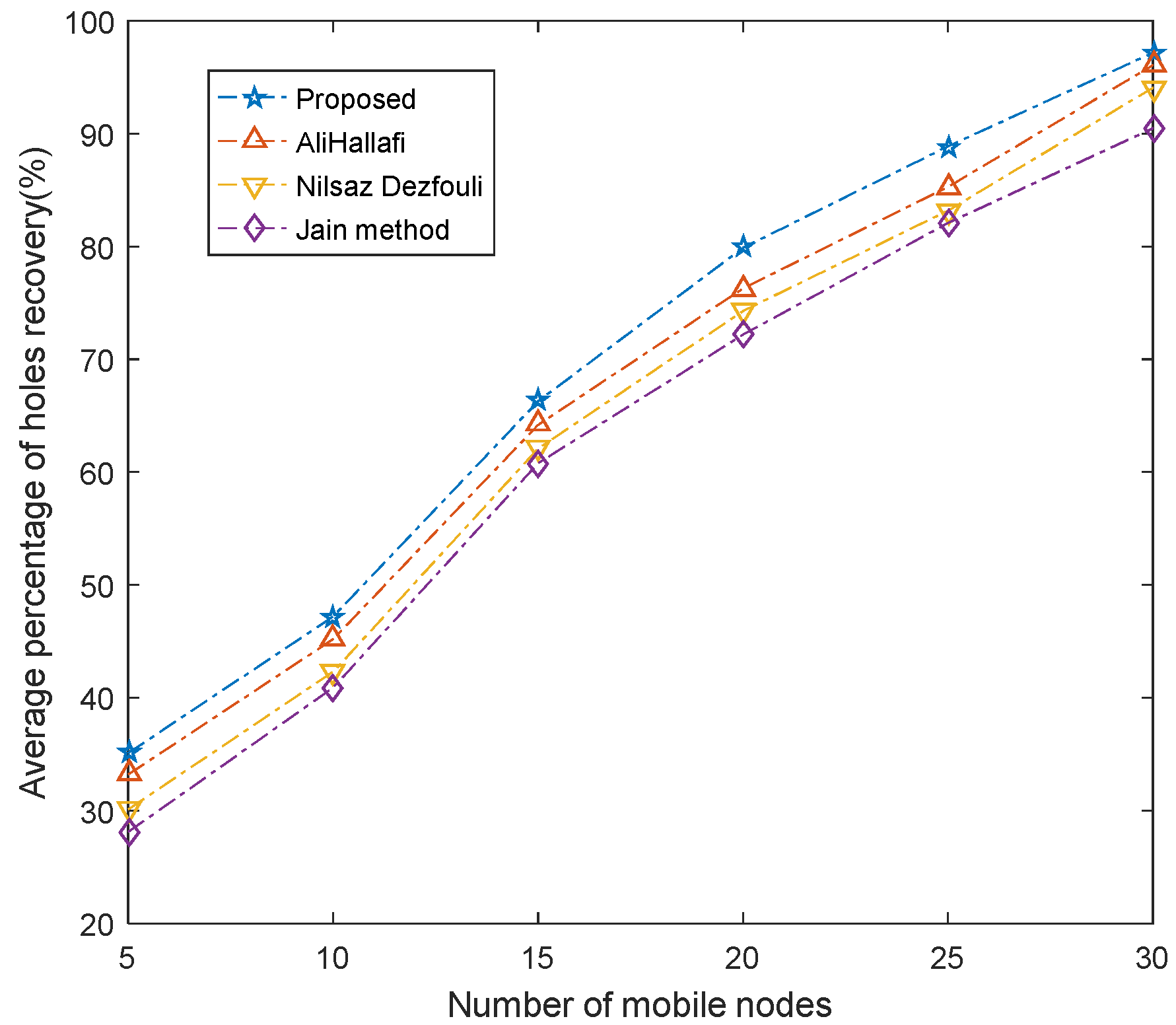
5.3. Average Percentage of Holes Repaired
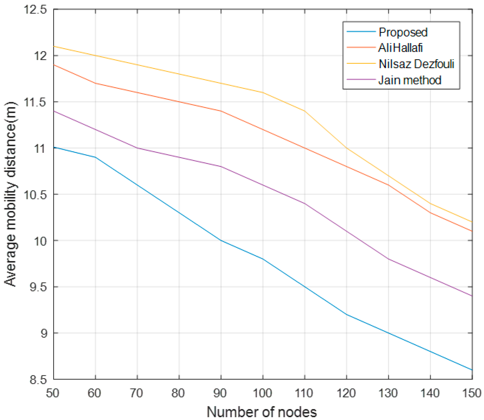
5.4. Average Mobility Distance of Mobile Nodes
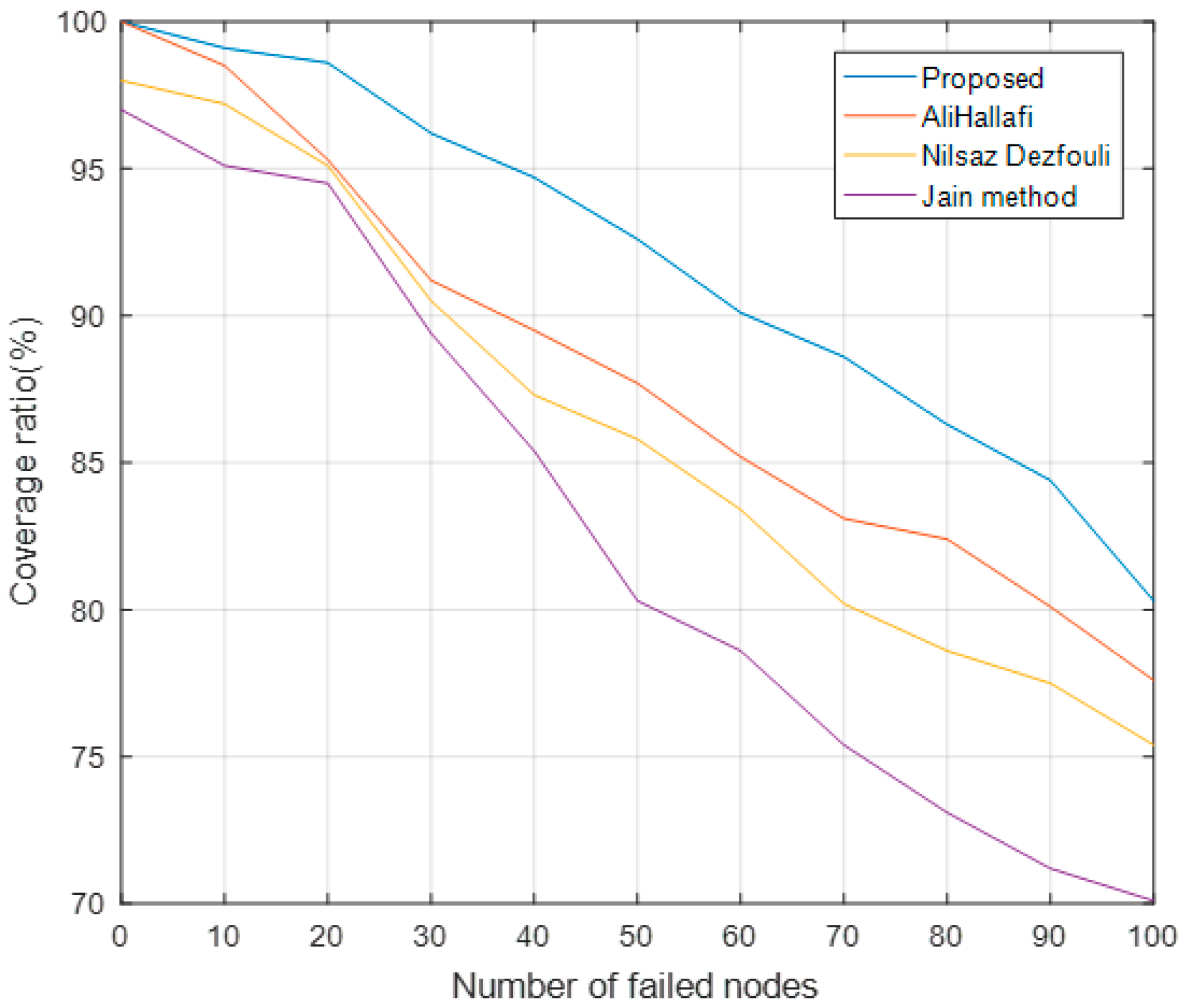
5.5. Coverage Ratio with Different Number of Failed Nodes
5.6. Average Coverage at Different Simulation Times

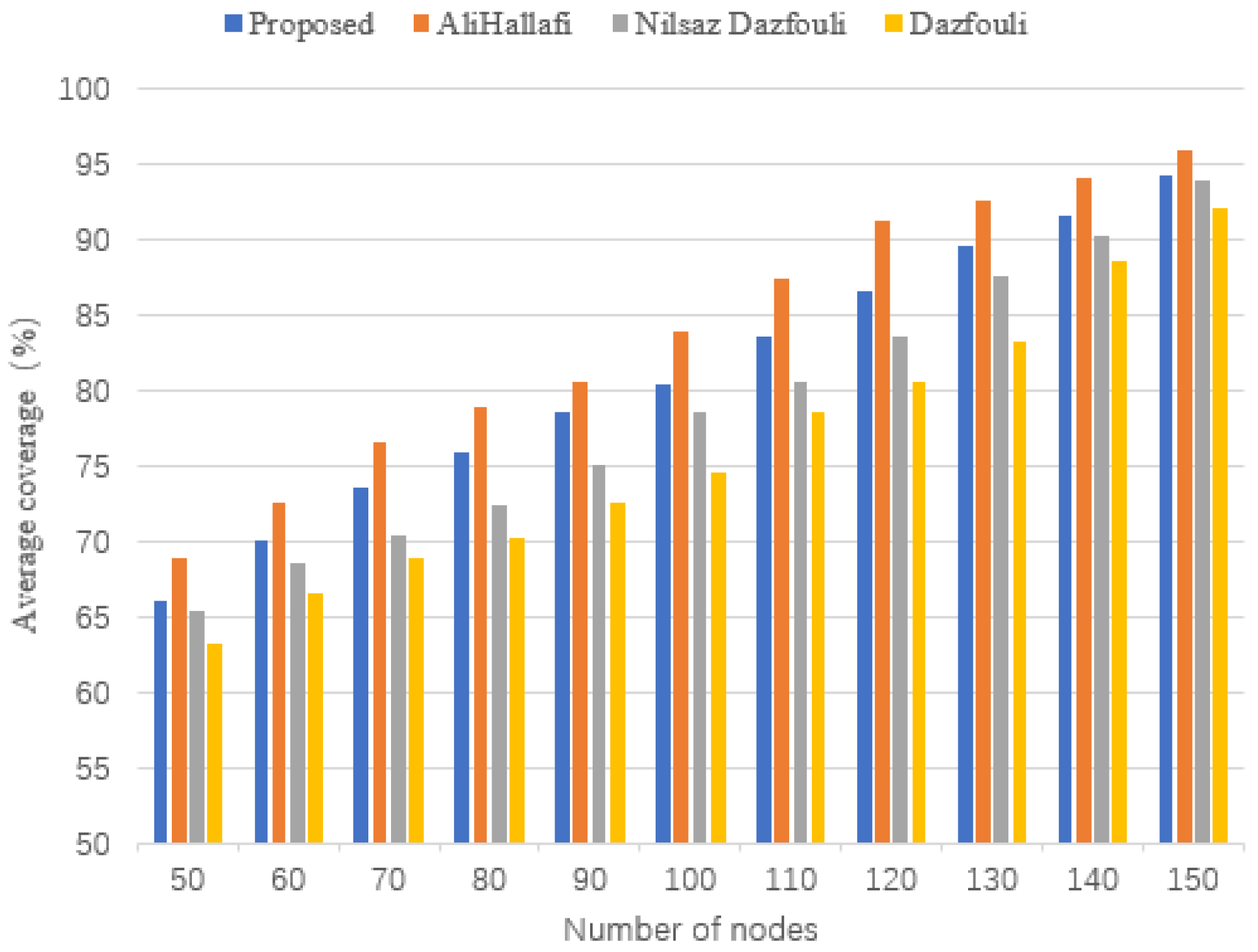
5.7. Average Coverage
6. Conclusions
Author Contributions
Funding
Institutional Review Board Statement
Informed Consent Statement
Data Availability Statement
Conflicts of Interest
References
- Qu, S.; Zhao, L.; Xiong, Z. Cross-layer congestion control of wireless sensor networks based on fuzzy sliding mode control. Neural Comput. Appl. 2020, 32, 13505–13520. [Google Scholar] [CrossRef]
- Rathinam, D.D.K.; Surendran, D.; Shilpa, A.; Grace, A.S.; Sherin, J. Modern Agriculture Using Wireless Sensor Network (WSN). In Proceedings of the 5th International Conference on Advanced Computing & Communication Systems (ICACCS), Coimbatore, India, 15–16 March 2019; pp. 515–519. [Google Scholar]
- Deebak, B.D.; Al-Turjman, F. A hybrid secure routing and monitoring mechanism in IoT-based wireless sensor networks. Ad Hoc Netw. 2020, 97, 102022. [Google Scholar]
- Singh, A.; Kumar, D.; Hötzel, J. IoT Based information and communication system for enhancing underground mines safety and productivity: Genesis, taxonomy and open issues. Ad Hoc Netw. 2018, 78, 115–129. [Google Scholar] [CrossRef]
- Boukerche, A.; Sun, P. Connectivity and coverage based protocols for wireless sensor networks. Ad Hoc Netw. 2018, 80, 54–69. [Google Scholar] [CrossRef]
- Ahmadi, H.; Viani, F.; Bouallegue, R. An accurate prediction method for moving target localization and tracking in wireless sensor networks. Ad Hoc Netw. 2018, 70, 14–22. [Google Scholar] [CrossRef]
- Sun, G.; Liu, Y.; Yang, M.; Wang, A.; Liang, S.; Zhang, Y. Coverage optimization of VLC in smart homes based on improved cuckoo search algorithm. Comput. Netw. 2017, 116, 63–78. [Google Scholar] [CrossRef]
- Hajjej, F.; Hamdi, M.; Ejbali, R.; Zaied, M. A distributed coverage hole recovery approach based on reinforcement learning for Wireless Sensor Networks. Ad Hoc Netw. 2020, 101, 102082. [Google Scholar] [CrossRef]
- Hallafi, A.; Barati, A.; Barati, H. A distributed energy-efficient coverage holes detection and recovery method in wireless sensor networks using the grasshopper optimization algorithm. J. Ambient. Intell. Humaniz. Comput. 2022, 14, 13697–13711. [Google Scholar] [CrossRef]
- Verma, M.; Sharma, S. A Greedy Approach for Coverage Hole Detection and Restoration in Wireless Sensor Networks. Wirel. Pers. Commun. 2018, 101, 75–86. [Google Scholar] [CrossRef]
- Singh, P.; Chen, Y.-C. Sensing coverage hole identification and coverage hole healing methods for wireless sensor networks. Wirel. Netw. 2019, 26, 2223–2239. [Google Scholar] [CrossRef]
- Nguyen, D.T.; Nguyen, N.P.; Thai, M.T.; Helal, A. An optimal algorithm for coverage hole healing in hybrid sensor networks. In Proceedings of the 7th International Wireless Communications and Mobile Computing Conference, Istanbul, Turkey, 4–8 July 2011; pp. 494–499. [Google Scholar]
- Elhabyan, R.; Shi, W.; St-Hilaire, M. Coverage protocols for wireless sensor networks: Review and future directions. J. Commun. Netw. 2019, 21, 45–60. [Google Scholar] [CrossRef]
- Hanh, N.T.; Binh, H.T.T.; Hoai, N.X.; Palaniswami, M.S. An efficient genetic algorithm for maximizing area coverage in wireless sensor networks. Inf. Sci. 2019, 488, 58–75. [Google Scholar] [CrossRef]
- Dezfuli, N.N.; Barati, H. Distributed energy efficient algorithm for ensuring coverage of wireless sensor networks. IET Commun. 2019, 13, 578–584. [Google Scholar] [CrossRef]
- Xiong, A.; Hou, R.; Zhou, L.; Xing, G.; Zeng, D. K-means++ and Reinforcement Learning-Based Clustering Method to Achieve Energy Efficiency in Underwater Acoustic Sensor Networks. In Proceedings of the 2023 IEEE International Conference on Parallel & Distributed Processing with Applications, Big Data & Cloud Computing, Sustainable Computing & Communications, Social Computing & Networking (ISPA), Wuhan, China, 21–24 December 2023; pp. 50–55. [Google Scholar]
- Manju; Singh, S.; Kumar, S.; Nayyar, A.; Al-Turjman, F.; Mostarda, L. Proficient QoS-Based Target Coverage Problem in Wireless Sensor Networks. IEEE Access 2020, 8, 74315–74325. [Google Scholar] [CrossRef]
- Sharmin, N.; Karmaker, A.; Lambert, W.L.; Alam, M.S.; Shawkat, M.S.A. Minimizing the Energy Hole Problem in Wireless Sensor Networks: A Wedge Merging Approach. Sensors 2020, 20, 277. [Google Scholar] [CrossRef]
- Chowdhuri, R.; Barma, D. Node position estimation based on optimal clustering and detection of coverage hole in wireless sensor networks using hybrid deep reinforcement learning. J. Supercomput. 2023, 79, 20845–20877. [Google Scholar] [CrossRef]
- Chowdhuri, R.; Barma, D. Enhancing Network Reliability: Exploring Effective Strategies for Coverage-Hole Analysis and Patching in Wireless Sensor Networks. Wirel. Pers. Commun. 2024, 134, 487–517. [Google Scholar] [CrossRef]
- Lu, X.; Wei, Y.; Wu, Q.; Yang, C.; Li, D.; Zhang, L.; Zhou, Y. A Coverage Hole Patching Algorithm for Heterogeneous Wireless Sensor Networks. Electronics 2022, 11, 3563. [Google Scholar] [CrossRef]
- Zhou, S.; Wu, M.-Y.; Shu, W. Finding optimal placements for mobile sensors: Wireless sensor network topology adjustment. In Proceedings of the IEEE 6th Circuits and Systems Symposium on Emerging Technologies: Frontiers of Mobile and Wireless Communication, Shanghai, China, 31 May–2 June 2004; pp. 529–532. [Google Scholar]
- Gou, P.; Mao, G.; Zhang, F.; Jia, X. Reconstruction of coverage hole model and cooperative repair optimization algorithm in heterogeneous wireless sensor networks. Comput. Commun. 2020, 153, 614–625. [Google Scholar] [CrossRef]
- Li, Q.; Liu, N. Monitoring area coverage optimization algorithm based on nodes perceptual mathematical model in wireless sensor networks. Comput. Commun. 2020, 155, 227–234. [Google Scholar] [CrossRef]
- Khalifa, B.; Khedr, A.M.; Al Aghbari, Z. A Coverage Maintenance Algorithm for Mobile WSNs With Adjustable Sensing Range. IEEE Sens. J. 2020, 20, 1582–1591. [Google Scholar] [CrossRef]
- Tarnaris, K.; Preka, I.; Kandris, D.; Alexandridis, A. Coverage and k-Coverage Optimization in Wireless Sensor Networks Using Computational Intelligence Methods: A Comparative Study. Electronics 2020, 9, 675. [Google Scholar] [CrossRef]
- Latif, K.; Javaid, N.; Ahmad, A.; Khan, Z.A.; Alrajeh, N.; Khan, M.I. On Energy Hole and Coverage Hole Avoidance in Underwater Wireless Sensor Networks. IEEE Sens. J. 2016, 16, 4431–4442. [Google Scholar] [CrossRef]
- Izadi, D.; Abawajy, J.; Ghanavati, S. An Alternative Node Deployment Scheme for WSNs. IEEE Sens. J. 2015, 15, 667–675. [Google Scholar] [CrossRef]
- Xiong, Y.; Chen, G.; Lu, M.; Wan, X.; Wu, M.; She, J. A Two-Phase Lifetime-Enhancing Method for Hybrid Energy-Harvesting Wireless Sensor Network. IEEE Sens. J. 2020, 20, 1934–1946. [Google Scholar] [CrossRef]
- Jain, J.K. A Coherent Approach for Dynamic Cluster-Based Routing and Coverage Hole Detection and Recovery in Bi-layered WSN-IoT. Wirel. Pers. Commun. 2020, 114, 519–543. [Google Scholar] [CrossRef]
- Rahmani, A.M.; Ali, S.; Malik, M.H.; Yousefpoor, E.; Yousefpoor, M.S.; Mousavi, A.; Khan, F.; Hosseinzadeh, M. An energy-aware and Q-learning-based area coverage for oil pipeline monitoring systems using sensors and Internet of Things. Sci. Rep. 2022, 12, 9638. [Google Scholar] [CrossRef]
- Karp, B. Greedy Perimeter Stateless Routing for Wireless Networks. In Proceedings of the 6th Annual International Conference on Mobile Computing and Networking, Boston, MA, USA, 6–11 August 2000; pp. 243–254. [Google Scholar]
- Tian, D.; Georganas, N.D. Connectivity maintenance and coverage preservation in wireless sensor networks. Ad Hoc Netw. 2005, 3, 744–761. [Google Scholar] [CrossRef]
- Heinzelman, W.R.; Chandrakasan, A.; Balakrishnan, H. Energy-efficient communication protocol for wireless microsensor networks. In Proceedings of the 33rd Annual Hawaii International Conference on System Sciences, Maui, HI, USA, 7 January 2000; p. 10. [Google Scholar]


| Coordinate | S1 | S2 | S3 | S4 | S5 | … | Sn | CoNO |
|---|---|---|---|---|---|---|---|---|
| (x1, y1) | 0 | 0 | 0 | 0 | 0 | 0 | 0 | |
| … | ||||||||
| (x40, y40) | 1 | 1 | 0 | 0 | 0 | 0 | 1 | |
| … | ||||||||
| (x100, y100) | 0 | 1 | 1 | 1 | 0 | 0 | 1 | |
| … | ||||||||
| (xk−1, yk−1) | 0 | 0 | 0 | 0 | 0 | 0 | 0 | |
| (xk, yk) | 0 | 0 | 0 | 0 | 0 | 0 | 0 |
| Symbol | Attribute | Value |
|---|---|---|
| O | monitoring area | 200 ∗ 200 m2 |
| Deploy | deployment method | Random |
| L | length of the network | 200 |
| Si | a sensor node | 180 |
| Aij | represents a unit | |
| C | number of units | Depends on the number of nodes |
| Rs | sensor i sensing radius | 30 m |
| Rc | sensor i communication radius | 60 m |
| Vi | movement speed of sensor i | 20 m/s |
| n | number of static sensor nodes | 150 |
| m | number of mobile sensor nodes | 30 |
| Em | initial energy of the mobile node | 5 J |
| Ec | mobile energy consumption | 0.1 J/m |
| SIM | simulation time | 150 s |
Disclaimer/Publisher’s Note: The statements, opinions and data contained in all publications are solely those of the individual author(s) and contributor(s) and not of MDPI and/or the editor(s). MDPI and/or the editor(s) disclaim responsibility for any injury to people or property resulting from any ideas, methods, instructions or products referred to in the content. |
© 2025 by the authors. Licensee MDPI, Basel, Switzerland. This article is an open access article distributed under the terms and conditions of the Creative Commons Attribution (CC BY) license (https://creativecommons.org/licenses/by/4.0/).
Share and Cite
Li, H.; Sun, S.; Dong, C.; Qi, Q.; Zhao, C.; Fu, Z.; Yu, P.; Liu, J. Coverage Hole Recovery in Hybrid Sensor Networks Based on Key Perceptual Intersections for Emergency Communications. Sensors 2025, 25, 4217. https://doi.org/10.3390/s25134217
Li H, Sun S, Dong C, Qi Q, Zhao C, Fu Z, Yu P, Liu J. Coverage Hole Recovery in Hybrid Sensor Networks Based on Key Perceptual Intersections for Emergency Communications. Sensors. 2025; 25(13):4217. https://doi.org/10.3390/s25134217
Chicago/Turabian StyleLi, He, Shixian Sun, Chuang Dong, Qinglei Qi, Cong Zhao, Zufeng Fu, Peng Yu, and Jiajia Liu. 2025. "Coverage Hole Recovery in Hybrid Sensor Networks Based on Key Perceptual Intersections for Emergency Communications" Sensors 25, no. 13: 4217. https://doi.org/10.3390/s25134217
APA StyleLi, H., Sun, S., Dong, C., Qi, Q., Zhao, C., Fu, Z., Yu, P., & Liu, J. (2025). Coverage Hole Recovery in Hybrid Sensor Networks Based on Key Perceptual Intersections for Emergency Communications. Sensors, 25(13), 4217. https://doi.org/10.3390/s25134217