
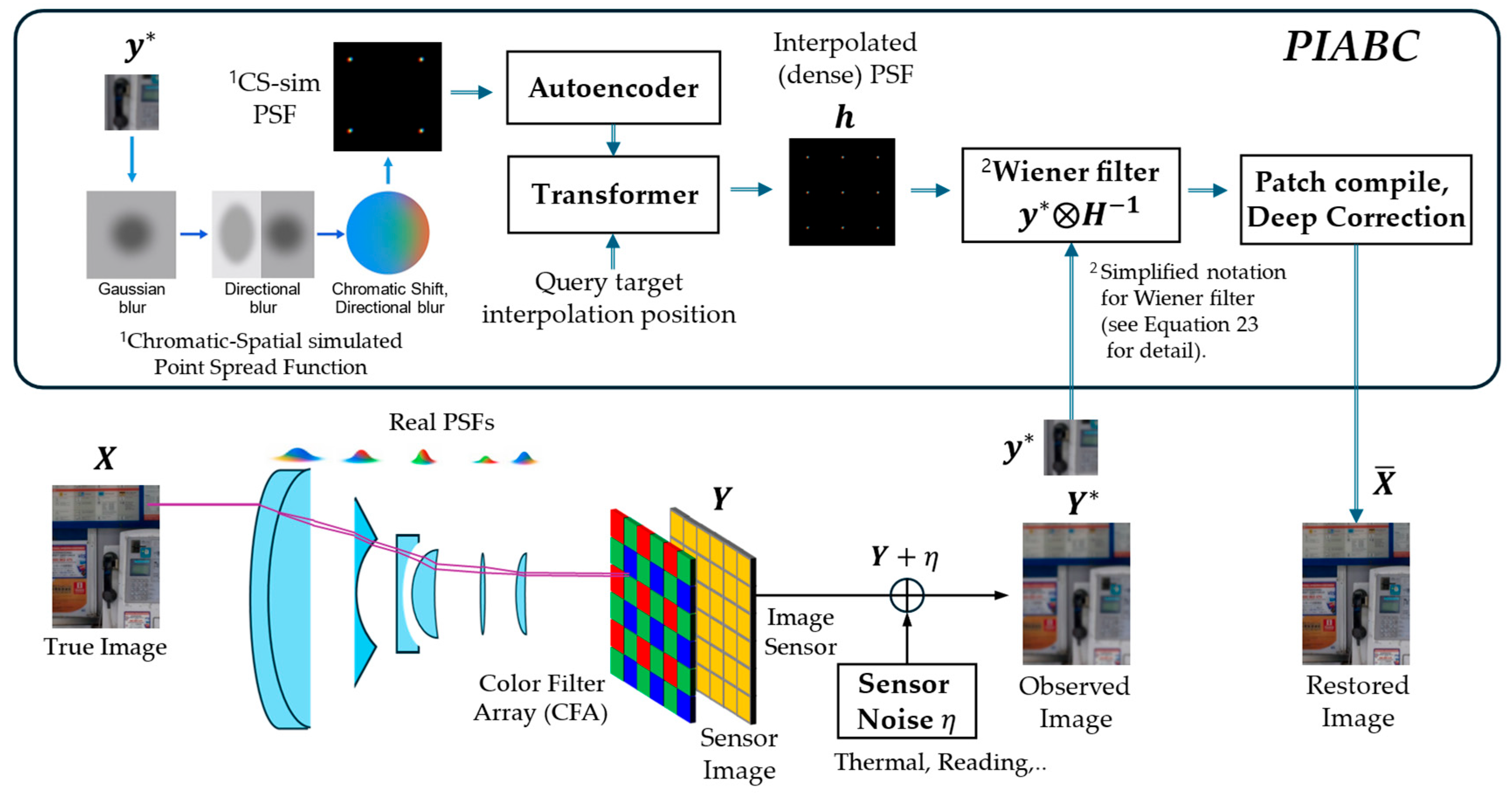
PIABC: Point Spread Function Interpolative Aberration Correction


Abstract
1. Introduction
- Dense PSF representation interpolation using a shallow transformer;
- Wiener filtering with the interpolated PSFs;
- Spatial signal refinement through a deep residual U-Net.
- Dense PSF estimation through pixel-level PSF embedding;
- Autoencoder (AE) latent space PSF interpolation using learned representations;
- Cross-attention-based PSF refinement between patches;
- Long-range dependency capture ensuring global correction coherence.
2. Relative Works
2.1. Interrelation Between Optical Aberration Correction and System-Level Artifacts
2.2. Correction of Sensor-Induced Degradation and Optical Aberrations
2.3. Comparison with Existing PSF Modeling Approaches
3. Methods
- Formulation;
- Generating chromatic-spatial simulated PSF (CS-sim PSF);
- PSF interpolation on latent space using AE and vision transformer (ViT);
- Patch-wise image restoration using a Wiener filter;
- Patch assembling and full-image compilation;
- Deep residual correction using a residual U-Net (Res U-Net);
- Training objects and loss functions.
3.1. Formulation
3.2. Generating Chromatic-Spatail Simulated PSF (CS-sim PSF)
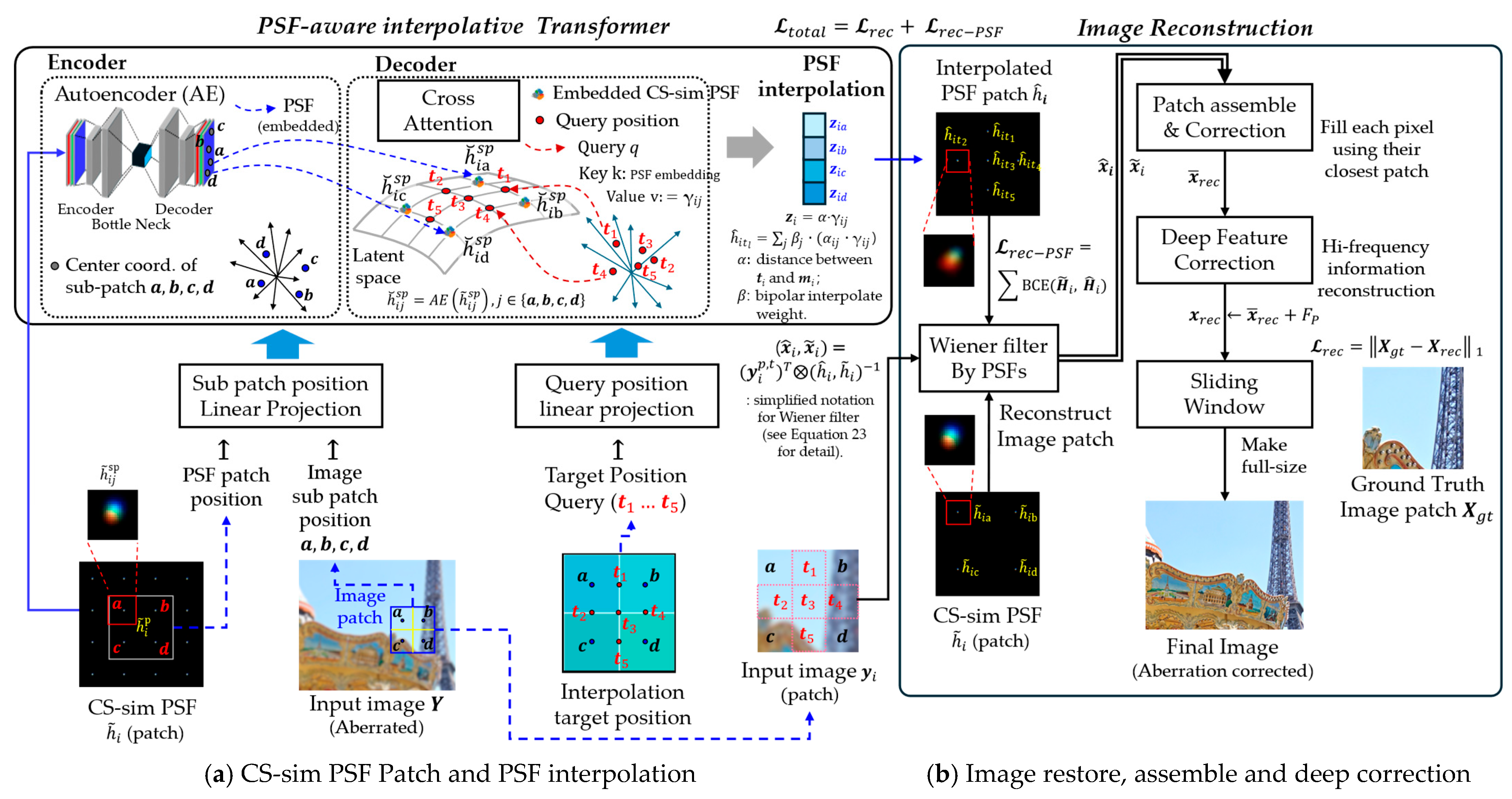
3.3. Spatially Varying PSF Interpolation for Noise Reduction Using Deep Learning
3.3.1. Query Patch Configuration for Spatially Varying PSF Interpolation

3.3.2. PSF Patch Embedding with Autoencoder
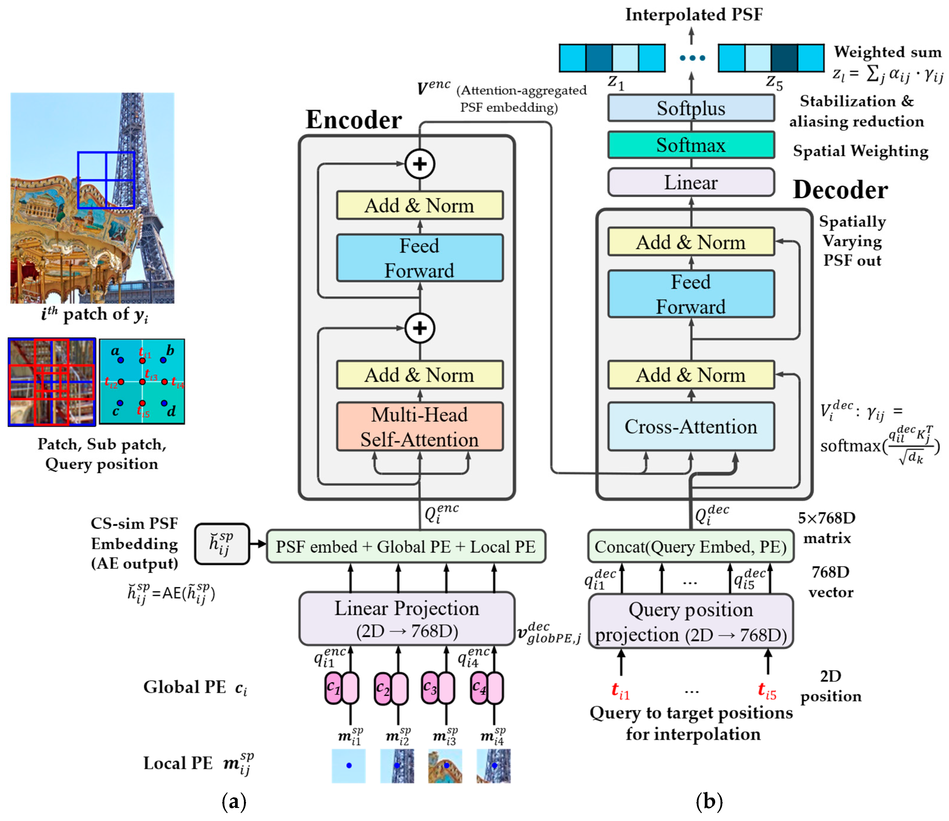
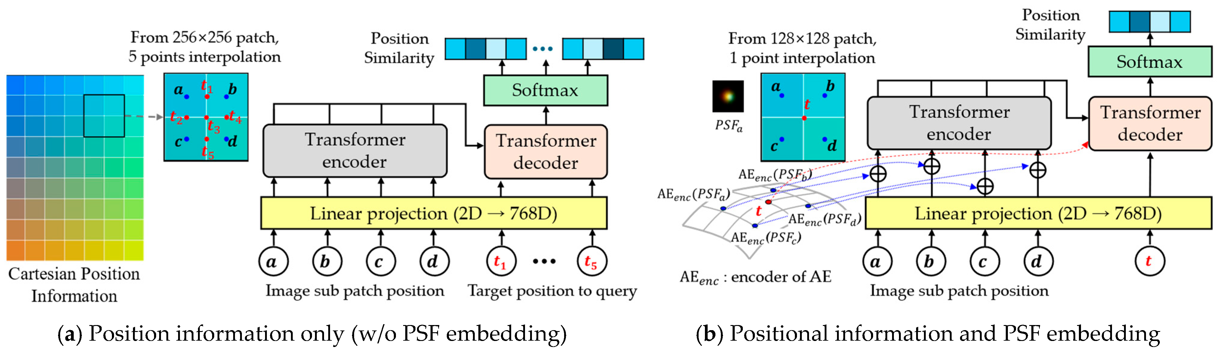
3.3.3. Transformer-Based PSF Interpolation for Enhanced Accuracy
- Encoder: Applies self-attention to aggregated PSF embeddings with positional encodings. Each sub-patch PSF embedding is combined with local position embedding and global position embedding . The encoder input query is then formulated as:where indexes sub-patches within the PSF patch . Although layer normalization (LN) is not explicitly shown here, it is applied internally within the transformer encoder block. This step preserves both local and global spatial context in the encoder tokens. denotes the center coordinates of each sub-patch.
- Decoder: For each target query position , the decoder query vector vector is computed as:This decoder query interacts with the encoder outputs via a cross-attention block, producing attention weights and aggregated latent features :where represents the encoder key vector, and is the key dimension. This mechanism captures the contribution of each sub-patch embedding to the interpolation target.
- Position Similarity: Position similarity between the query position and each sub-patch center is defined as:where indexes the neighboring sub-patches. This term quantifies the geometric proximity between the interpolation target and each sub-patch center.
- Latent Aggregation: The position similarity and attention weights are combined to produce the weighted latent feature:
- Interpolation Step: The final interpolated PSF at the query position is then obtained as:where denotes the bilinear interpolation weight derived from the relative distances between the target position and the sub-patch centers :Finally, a linear projection is applied to to generate the interpolated PSF :
3.4. Image Restoration Using Image Restoration Using Wiener Filtering and Deep Correction
3.4.1. Patch Image Restoration Using Wiener Filter
3.4.2. Patch Assembly Using Transformer-Interpolated PSFs
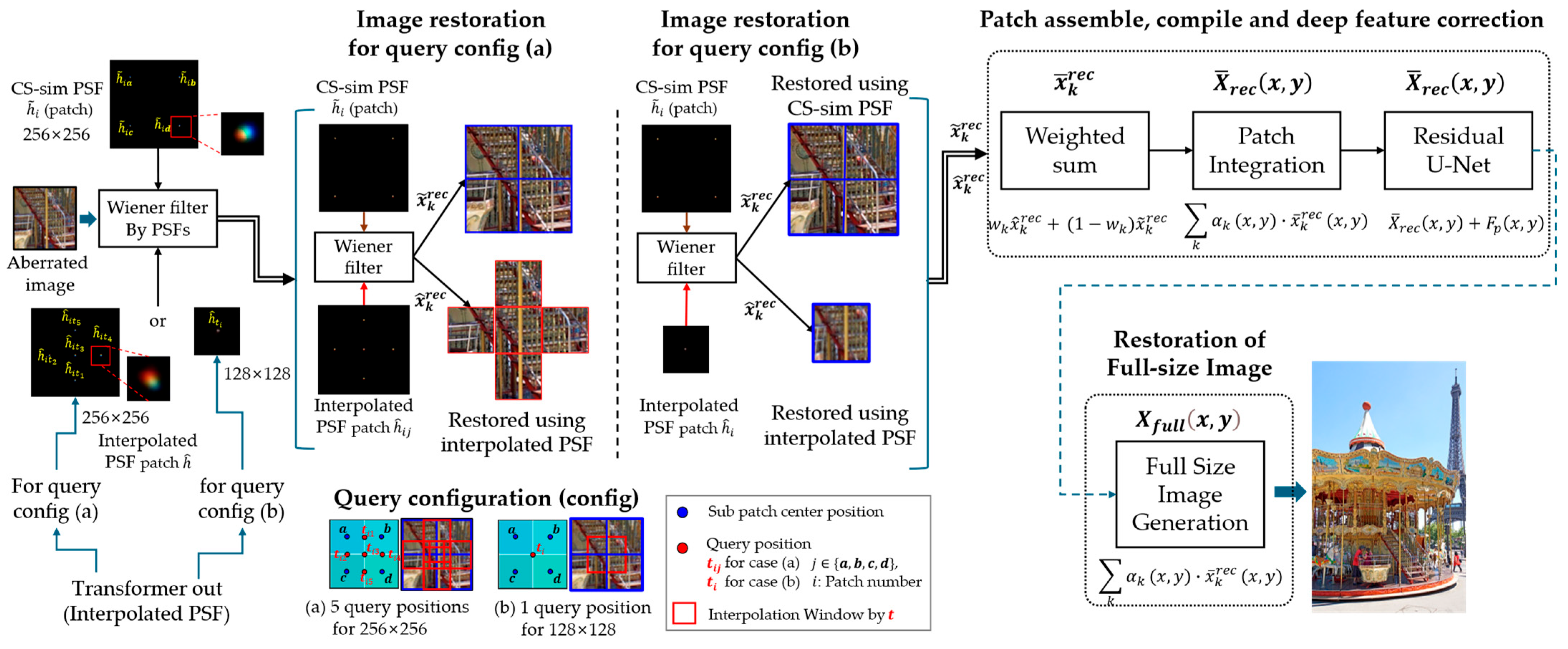
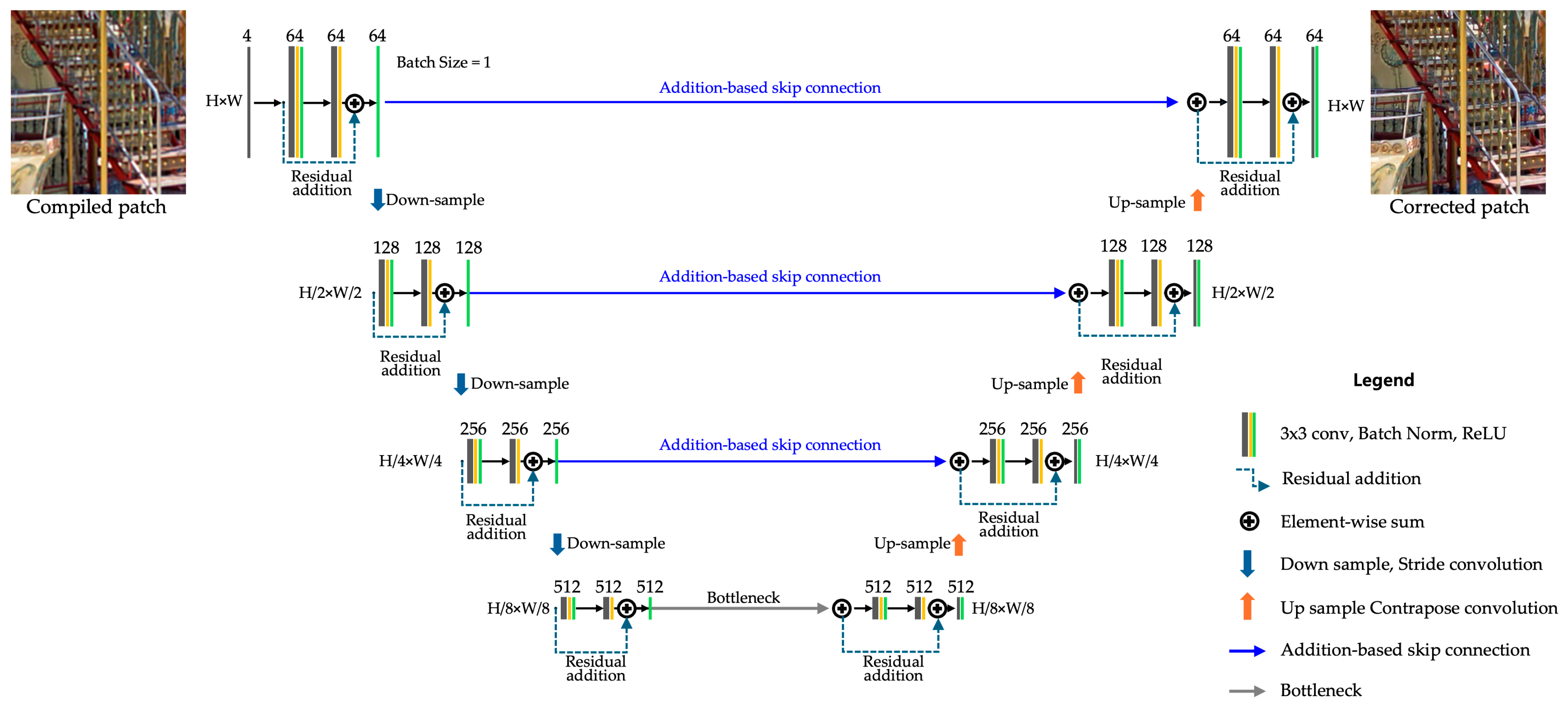
3.4.3. Deep Feature Correction Using Residual U-Net
- Enhanced Decoder with Residual Additions: Residual connections are added within the decoder to improve feature refinement and gradient flow stability.
3.5. Training Objects and Loss Functions
4. Experiments and Results
4.1. Experimental Setup
4.1.1. Training Dataset
4.1.2. Training Parameter Configuration
4.1.3. Residual U-Net Configuration
- Loss Function: -norm loss;
- Optimizer: Adam optimizer;
- Learning Rate: 0.0001;
- Activation Function: ReLU;
- Batch Size (B): 1.
4.1.4. Chromatic-Spatial Simulated PSF (CS-sim PSF) Setup
- Gaussian blur applied uniformly using an isotropic Gaussian function;
- Radial anisotropic transformations to simulate spatially varying distortions;
- Wavelength-dependent distortion modeling (e.g., or ) with varying inner and outer sigma intensities.
4.1.5. Fine-Tuning Configuration
4.1.6. K Parameter Pre-Evaluation for Robust Filtering
4.1.7. Computing Environment
4.2. Benchmark Test
4.2.1. Performance Metrics
4.2.2. Benchmark Models
- Wiener-Prior UABC-net (adapted from Li et al. [9]): The original UABC uses a PSF-aware deep network, pre-trained on Zemax-simulated PSFs and fine-tuned for specific lenses. We replaced PSF reconstruction with regulated Wiener filtering using synthetic PSFs, keeping the U-Net refinement to reduce artifacts. This preserves the PSF-aware correction focus;
- Patch-based Deformable ResU-net (adapted from Chen et al. [10]): Chen et al. (2021) proposes an imaging simulation system that computes spatially variant PSFs using lens data and raytracing for post-processing, paired with a spatial-adaptive CNN featuring Deformable ResBlocks. We preserve the Deformable ResBlock’s role in handling non-uniform distortions. This ensures the method’s spatial adaptability is retained.
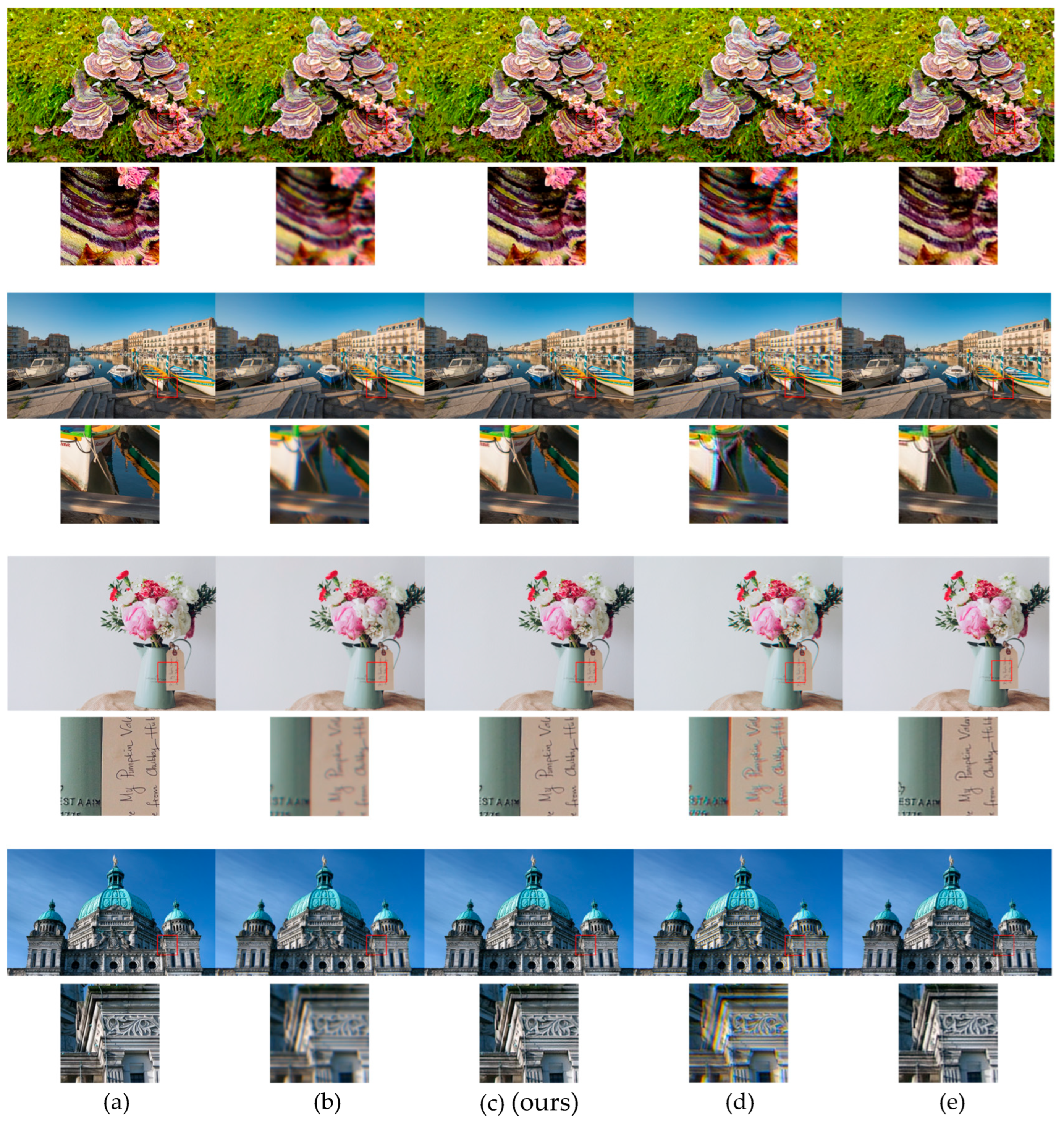
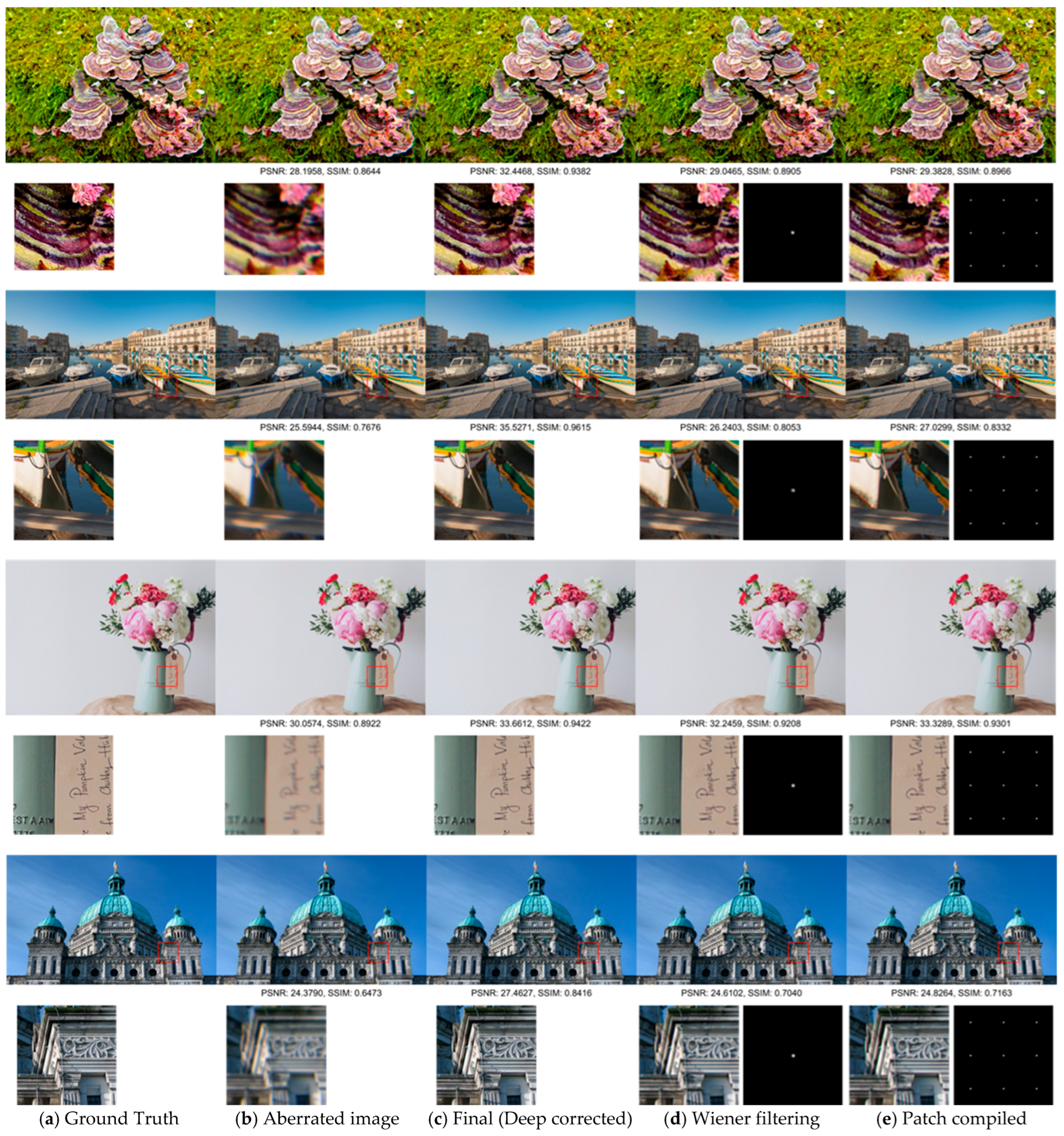
4.2.3. Quantitative and Qualitative Comparison on DIV2K Dataset
4.2.4. Quantitative and Qualitative Comparison Using RealSR-V3 Canon 5D3 Dataset
4.3. Ablation Study
4.3.1. Analysis of Stage-Wise Effects and Embedding on DIV2K Dataset
- Applying the Wiener filter to the aberrated image improves PSNR and SSIM by 1.4123 dB and 0.0787, respectively.
- Replacing observed PSFs with interpolated PSFs yields a marginal improvement (ΔPSNR = 0.1373 dB, ΔSSIM = 0.0024), suggesting interpolation accuracy aligns closely with actual measurements.
- Compared to using only observed PSFs, the residual U-Net adds a substantial gain of 5.479 dB in PSNR and 0.1161 in SSIM, highlighting the effectiveness of deep refinement.
4.3.2. Stage-Wise PSF Modeling and Fine-Tuning Effects on DIV2K Dataset
4.3.3. Stage-Wise Fine-Tuning Effects on RealSR-V3 Canon 5D3 Dataset
4.4. Results
4.4.1. Performance on DIV2K (Synthetic LR)
4.4.2. Performance on RealSR-V3 (Natural LR)
4.4.3. Comparative Analysis and Implications
5. Discussion
6. Conclusions
7. Limitations and Future Work
Author Contributions
Funding
Institutional Review Board Statement
Informed Consent Statement
Data Availability Statement
Acknowledgments
Conflicts of Interest
Appendix A. K Value Sensitivity Analysis for Robust Wiener Filtering

| Dataset | K Value | PSNR (dB) | SSIM |
|---|---|---|---|
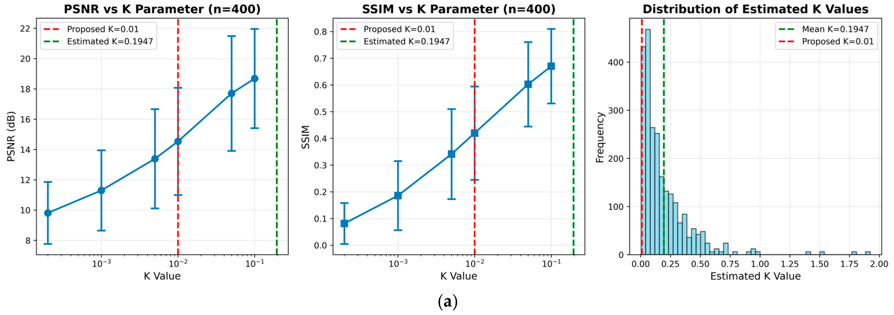
| DIV2K HR Train | 0.0002 | 9.81 ± 2.04 | 0.0815 ± 0.0765 |
| 0.0010 | 11.30 ± 2.65 | 0.1857 ± 0.1294 | |
| 0.0050 | 13.39 ± 3.28 | 0.3413 ± 0.1684 | |
| 0.0100 | 14.53 ± 3.54 | 0.4197 ± 0.1747 | |
| 0.0500 | 17.70 ± 3.79 | 0.6026 ± 0.1580 | |
| 0.1000 | 18.69 ± 3.20 | 0.6703 ± 0.1397 | |
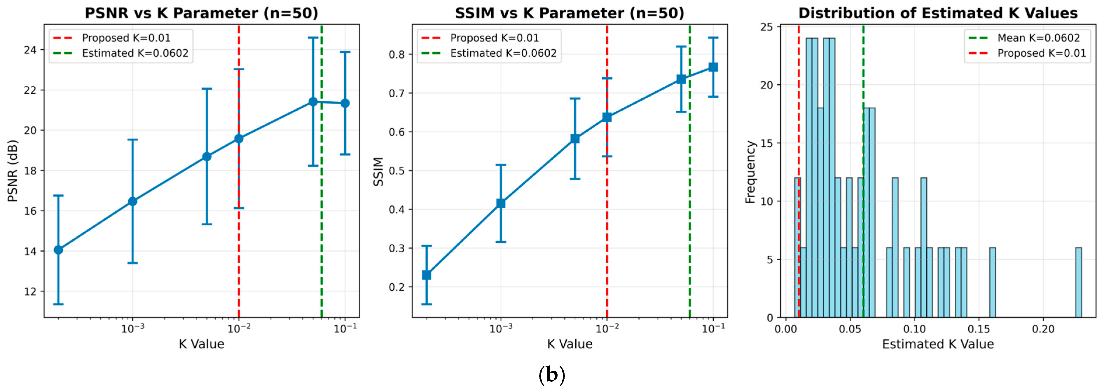
| RealSR (V3) Canon 2 LR | 0.0002 | 14.06 ± 2.70 | 0.2305 ± 0.0754 |
| 0.0010 | 16.47 ± 3.06 | 0.4152 ± 0.0994 | |
| 0.0050 | 18.69 ± 3.37 | 0.5819 ± 0.1038 | |
| 0.0100 | 19.58 ± 3.45 | 0.6372 ± 0.1006 | |
| 0.0500 | 21.42 ± 3.18 | 0.7355 ± 0.0843 | |
| 0.1000 | 21.34 ± 2.54 | 0.7664 ± 0.0763 |
| Dataset | Optimal K | K = 0.01 Performance | Deviation Factor |
|---|---|---|---|
| DIV2K HR Train | 0.1947 | PSNR: 14.53 ± 3.54 dB, SSIM: 0.4197 ± 0.1747 | 19.5× |
| RealSR (V3) Canon 2 LR | 0.0602 | PSNR: 19.58 ± 3.45 dB, SSIM: 0.6372 ± 0.1006 | 6.0× |
- Validity of K = 0.01:
- The histogram of MMSE-estimated K values shown in Figure A1 (a, right) and Figure A1 (b, right) shows a dominant concentration in the range of 0.02 to 0.12, with a mean of 0.1947 and 0.0602, respectively. This supports the view that our empirical choice (K = 0.01) is a conservative yet well-grounded setting.
- Our empirical choice of K = 0.01 lies near the lower bound of this range, representing a conservative yet reasonable selection grounded in signal preservation.
- Sensitivity Trends:
- As K increases from 0.0002 to 0.1000, both PSNR and SSIM improve steadily:
- –
- DIV2K: PSNR improves from 9.81 dB to 18.69 dB, SSIM from 0.0815 to 0.6703,
- –
- RealSR: PSNR improves from 14.06 dB to 21.34 dB, SSIM from 0.2305 to 0.7664.
- It shows a robust, quasi-logarithmic relationship between K and restoration quality.
- Robustness of Fixed K:
- Despite not being the MMSE-optimal, K = 0.01 yields strong intermediate performance across datasets.
- RealSR shows only 1.76 dB loss (vs. optimal K); DIV2K shows 4.16 dB loss.
- The consistent error bar trends validate the reliability of this fixed setting across real and synthetic domains.
Appendix B. Illustration of CS-sim-PSF

References
- Kondepudy, R.; Healey, G. Using Moment Invariants to Analyze 3-D Color Textures. In Proceedings of the 1st International Conference on Image Processing, Austin, TX, USA, 13–16 November 1994; Volume 2, pp. 61–65. [Google Scholar]
- Foi, A.; Trimeche, M.; Katkovnik, V.; Egiazarian, K. Practical Poissonian-Gaussian Noise Modeling and Fitting for Sin-gle-Image Raw-Data. IEEE Trans. Image Process. 2008, 17, 1737–1754. [Google Scholar] [CrossRef] [PubMed]
- El Gamal, A.; Eltoukhy, H. CMOS Image Sensors. IEEE Circuits Devices Mag. 2005, 21, 6–20. [Google Scholar] [CrossRef]
- Zhang, C.; Li, Y.; Wang, J.; Hao, P. Universal Demosaicking of Color Filter Arrays. IEEE Trans. Image Process. 2016, 25, 5173–5186. [Google Scholar] [CrossRef]
- Tian, J.; Chen, L. Adaptive Multi-Focus Image Fusion Using a Wavelet-Based Statistical Sharpness Measure. Signal Process. 2012, 92, 2137–2146. [Google Scholar] [CrossRef]
- Hasinoff, S.W.; Durand, F.; Freeman, W.T. Noise-Optimal Capture for High Dynamic Range Photography. In Proceedings of the 2010 IEEE Computer Society Conference on Computer Vision and Pattern Recognition, San Francisco, CA, USA, 13–18 June 2010; pp. 553–560. [Google Scholar]
- Mildenhall, B.; Barron, J.T.; Chen, J.; Sharlet, D.; Ng, R.; Carroll, R. Burst Denoising with Kernel Prediction Networks. In Proceedings of the 2018 IEEE/CVF Conference on Computer Vision and Pattern Recognition, Salt Lake City, UT, USA, 18–23 June 2018; pp. 2502–2510. [Google Scholar]
- Sitzmann, V.; Diamond, S.; Peng, Y.; Dun, X.; Boyd, S.; Heidrich, W.; Heide, F.; Wetzstein, G. End-to-End Optimization of Optics and Image Processing for Achromatic Extended Depth of Field and Super-Resolution Imaging. ACM Trans. Graph. 2018, 37, 114. [Google Scholar] [CrossRef]
- Li, X.; Suo, J.; Zhang, W.; Yuan, X.; Dai, Q. Universal and Flexible Optical Aberration Correction Using Deep-Prior Based Deconvolution. In Proceedings of the 2021 IEEE/CVF International Conference on Computer Vision (ICCV), Montreal, QC, Canada, 10–17 October 2021; pp. 2593–2601. [Google Scholar]
- Chen, S.; Feng, H.; Pan, D.; Xu, Z.; Li, Q.; Chen, Y. Optical Aberration Correction in Postprocessing Using Imaging Simulation. ACM Trans. Graph. 2021, 40, 192. [Google Scholar] [CrossRef]
- Zhang, L.; Zhang, H.; Shen, H.; Li, P. A Super-Resolution Reconstruction Algorithm for Surveillance Images. Signal Process. 2010, 90, 848–859. [Google Scholar] [CrossRef]
- Heide, F.; Steinberger, M.; Tsai, Y.-T.; Rouf, M.; Pająk, D.; Reddy, D.; Gallo, O.; Liu, J.; Heidrich, W.; Egiazarian, K.; et al. FlexISP: A Flexible Camera Image Processing Framework. ACM Trans. Graph 2014, 33, 231. [Google Scholar] [CrossRef]
- Schuler, C.J.; Hirsch, M.; Harmeling, S.; Schölkopf, B. Learning to Deblur. Adv. Neural Inf. Process. Syst. 2014, 27, 1439–1451. [Google Scholar] [CrossRef]
- Shih, Y.; Guenter, B.; Joshi, N. Image Enhancement Using Calibrated Lens Simulations. In Computer Vision—ECCV 2012; Fitzgibbon, A., Lazebnik, S., Perona, P., Sato, Y., Schmid, C., Eds.; Lecture Notes in Computer Science; Springer: Berlin/Heidelberg, Germany, 2012; Volume 7575, pp. 42–56. ISBN 978-3-642-33764-2. [Google Scholar]
- Goodman, J.W. Introduction to Fourier Optics, 4th ed.; W. H. Freeman: New York, NY, USA, 2017; ISBN 978-1-319-11916-4. [Google Scholar]
- Kee, E.; Paris, S.; Chen, S.; Wang, J. Modeling and Removing Spatially-Varying Optical Blur. In Proceedings of the 2011 IEEE International Conference on Computational Photography (ICCP), Pittsburgh, PA, USA, 8–10 April 2011; pp. 1–8. [Google Scholar]
- Stallinga, S. Accuracy of the Gaussian Point Spread Function Model in 2D Localization Microscopy. Opt. Express 2010, 18, 24461–24475. [Google Scholar] [CrossRef]
- Siddik, A.B.; Sandoval, S.; Voelz, D.; Boucheron, L.E.; Varela, L. Deep learning estimation of modified Zernike coefficients for image point spread functions. Opt. Express 2023, 31, 22903–22913. [Google Scholar] [CrossRef] [PubMed]
- Zhang, H.; Dai, Y.; Li, H.; Koniusz, P. Deep Stacked Hierarchical Multi-Patch Network for Image Deblurring. In Proceedings of the 2019 IEEE/CVF Conference on Computer Vision and Pattern Recognition (CVPR), Long Beach, CA, USA, 15–20 June 2019; pp. 5971–5979. [Google Scholar]
- Jing, L.; Zbontar, J.; LeCun, Y. Implicit Rank-Minimizing Autoencoder. Adv. Neural Inf. Process. Syst. 2020, 33, 14736–14746. [Google Scholar]
- Monakhova, K. Physics-Informed Machine Learning for Computational Imaging. Ph.D. Thesis, University of California, Berkeley, CA, USA, 2022. [Google Scholar]
- Chouzenoux, E.; Lau, T.T.K.; Lefort, C.; Pesquet, J.-C. Optimal Multivariate Gaussian Fitting with Applications to PSF Mod-eling in Two-Photon Microscopy Imaging. J. Math. Imaging Vis. 2019, 61, 1037–1050. [Google Scholar] [CrossRef]
- Jia, P.; Li, X.; Li, Z.; Wang, W.; Cai, D. Point Spread Function Modelling for Wide Field Small Aperture Telescopes with a Denoising Autoencoder. Mon. Not. R. Astron. Soc. 2020, 493, 651–660. [Google Scholar] [CrossRef]
- Schuler, C.J.; Hirsch, M.; Harmeling, S.; Schölkopf, B. Blind Correction of Optical Aberrations. In Computer Vision—ECCV 2012; Fitzgibbon, A., Lazebnik, S., Perona, P., Sato, Y., Schmid, C., Eds.; Lecture Notes in Computer Science; Springer: Berlin/Heidelberg, Germany, 2012; Volume 7574, pp. 187–200. ISBN 978-3-642-33711-6. [Google Scholar]
- Levin, A.; Weiss, Y.; Durand, F.; Freeman, W.T. Understanding and Evaluating Blind Deconvolution Algorithms. In Proceedings of the 2009 IEEE Conference on Computer Vision and Pattern Recognition, Miami, FL, USA, 20–25 June 2009; pp. 1964–1971. [Google Scholar]
- Yue, T.; Suo, J.; Wang, J.; Cao, X.; Dai, Q. Blind Optical Aberration Correction by Exploring Geometric and Visual Priors. In Proceedings of the 2015 IEEE Conference on Computer Vision and Pattern Recognition (CVPR), Boston, MA, USA, 7–12 June 2015; pp. 1684–1692. [Google Scholar]
- Li, W.; Yin, X.; Liu, Y.; Zhang, M. Computational Imaging through Chromatic Aberration Corrected Simple Lenses. J. Mod. Opt. 2017, 64, 2211–2220. [Google Scholar] [CrossRef]
- Zhang, Z.; Liu, Q.; Wang, Y. Road Extraction by Deep Residual U-Net. IEEE Geosci. Remote Sens. Lett. 2018, 15, 749–753. [Google Scholar] [CrossRef]
- Ronneberger, O.; Fischer, P.; Brox, T. U-Net: Convolutional Networks for Biomedical Image Segmentation. In Proceedings of the International Conference on Medical Image Computing and Computer-Assisted Intervention (MICCAI), Munich, Germany, 5–9 October 2015; Springer: Cham, Switzerland, 2015; pp. 234–241. [Google Scholar]
- Agustsson, E.; Timofte, R. NTIRE 2017 Challenge on Single Image Super-Resolution: Dataset and Study. In Proceedings of the 2017 IEEE Conference on Computer Vision and Pattern Recognition Workshops (CVPRW), Honolulu, HI, USA, 21–26 July 2017; pp. 1122–1131. [Google Scholar]
- Cai, J.; Zeng, H.; Yong, H.; Cao, Z.; Zhang, L. Toward Real-World Single Image Super-Resolution: A New Benchmark and a New Model. In Proceedings of the 2019 IEEE/CVF International Conference on Computer Vision (ICCV), Seoul, Republic of Korea, 27 October–2 November 2019; pp. 3086–3095. [Google Scholar]
- Diakogiannis, F.I.; Waldner, F.; Caccetta, P.; Wu, C. ResUNet-a: A Deep Learning Framework for Semantic Segmentation of Remotely Sensed Data. ISPRS J. Photogramm. Remote Sens. 2020, 162, 94–114. [Google Scholar] [CrossRef]
- Sun, K.; Xiao, B.; Liu, D.; Wang, J. Deep High-Resolution Representation Learning for Human Pose Estimation. In Proceedings of the 2019 IEEE/CVF Conference on Computer Vision and Pattern Recognition (CVPR), Long Beach, CA, USA, 16–20 June 2019; pp. 5693–5703. [Google Scholar] [CrossRef]
- Vaswani, A.; Shazeer, N.; Parmar, N.; Uszkoreit, J.; Jones, L.; Gomez, A.N.; Kaiser, Ł.; Polosukhin, I. Attention Is All You Need. Adv. Neural Inf. Process. Syst. 2017, 30, 5998–6008. [Google Scholar]
- Dosovitskiy, A.; Beyer, L.; Kolesnikov, A.; Weissenborn, D.; Zhai, X.; Unterthiner, T.; Dehghani, M.; Minderer, M.; Heigold, G.; Gelly, S.; et al. An Image Is Worth 16 × 16 Words: Transformers for Image Recognition at Scale. arXiv 2021, arXiv:2010.11929. [Google Scholar]
- Lee, S.H.; Lee, S.; Song, B.C. Vision Transformer for Small-Size Datasets. Sensors 2021, 21, 8448. [Google Scholar] [CrossRef]
- Saeed Rad, M.; Yu, T.; Musat, C.; Kemal Ekenel, H.; Bozorgtabar, B.; Thiran, J.-P. Benefiting from Bicubically Down-Sampled Images for Learning Real-World Image Super-Resolution. In Proceedings of the 2021 IEEE Winter Conference on Applications of Computer Vision (WACV), Waikoloa, HI, USA, 3–8 January 2021; pp. 1589–1598. [Google Scholar]
- Immerkær, J. Fast Noise Variance Estimation. Comput. Vis. Image Underst. 1996, 64, 300–302. [Google Scholar] [CrossRef]

| Stage | Input | Output | Dimension | Description |
|---|---|---|---|---|
| 1 | CS-sim PSF | Latent feature | Patch-level PSFs are flattened and embedded as feature vector. | |
| 2 | , , | Encoded vector | Encoder feature by combining AE output, local PE, and global PE. | |
| 3 | Query position | Decoder query vector | Decoder query tokens generated from 2D query positions. | |
| 4 | , | Aggregated latent | Attention aggregates latent features for each query from encoder outputs. | |
| 5 | Intermediate PSF | Decoder reshapes latent feature to generate interpolated PSF patch. | ||
| 6 | Final Interpolated PSF | Weighted sum and smoothing produce final interpolated PSF. |
| Component | Specification | Component | Specification | Component | Specification |
|---|---|---|---|---|---|
| Embedding Dimension | 768 | Activation Function | ReLU (PatchEmbed., MLP) | Batch Size | 1 |
| Encoder Layers | 12 | Normalization | LayerNorm (pre-norm config.) | Learning Rates | 10−4 (model params), 5 × 10⁻⁴ (spatial weight μ) |
| Decoder Layers | 6 | Positional Encoding | Learnable 2D (Cartesian coord.) | Optimizer | Adam, β₁ = 0.9, β₂ = 0.999 |
| Attention Heads | 12 | Initialization Scheme | Kaiming Uniform (PyTorch default) | Scheduler | StepLR, step size = 1000, decay γ = 0.9 |
| Feed-Forward Hidden Dimension | 1536 (MLP ratio = 2.0) | Iterations (global training) | 20,000 | Loss Function (see Equations (33)–(35)) | Total = Rec-PSF + Rec1 |
| Dropout Rate | 0.1 | Iterations (Fine-tuning) | 300 | Loss Weights | Uniform |
| Benchmark Model | (a) 256 × 256 Size Patch | (b) 128 × 128 Size Patch | ||||
|---|---|---|---|---|---|---|
| PSNR | SSIM | LPIPS | PSNR | SSIM | LPIPS | |
| Wiener-prior UABC-net 1 (4 global train) | 20.9233 | 0.6273 | 0.3730 | 21.3639 | 0.6418 | 0.3672 |
| Wiener-prior UABC-net 1 (5 local finetune) | 22.1003 | 0.6773 | 0.3427 | 25.4506 | 0.7867 | 0.3382 |
| Patch-based Deformable-net 2 (4 global train) | 26.3358 | 0.8147 | 0.2930 | 25.9587 | 0.8072 | 0.3066 |
| Patch-based Deformable-net 2 (5 local finetune) | 28.2875 | 0.8659 | 0.2571 | 27.5892 | 0.8527 | 0.2777 |
| PIABC (ours) (before 6 fine-tuning) 3 | 31.0044 | 0.9045 | 0.2036 | 31.4027 | 0.9082 | 0.2077 |
| PIABC (ours) (after 6 fine-tuning) 3 | 30.7611 | 0.9000 | 0.2077 | 31.2993 | 0.9079 | 0.2058 |
| Benchmark Model | (a) 256 × 256 Size Patch | (b) 128 × 128 Size Patch | ||||
|---|---|---|---|---|---|---|
| PSNR | SSIM | LPIPS | PSNR | SSIM | LPIPS | |
| Wiener-prior UABC-net 1 (4 global train) | 25.4307 | 0.7623 | 0.3730 | 24.5512 | 0.7465 | 0.3672 |
| Wiener-prior UABC-net 1 (5 local finetune) | 26.4300 | 0.8109 | 0.3427 | 26.3750 | 0.8157 | 0.3382 |
| Patch-based Deformable-net 2 (4 global train) | 28.0515 | 0.8450 | 0.2930 | 27.9809 | 0.8462 | 0.3066 |
| Patch-based Deformable-net 2 (5 local finetune) | 28.9409 | 0.8664 | 0.2571 | 29.2001 | 0.8733 | 0.2777 |
| PIABC (ours) (before 6 fine-tuning) 3 | 30.0258 | 0.8851 | 0.2143 | 30.5716 | 0.8935 | 0.2073 |
| PIABC (ours) (after 6 fine-tuning) 3 | 28.9128 | 0.8768 | 0.2208 | 30.1090 | 0.8872 | 0.2120 |
| Process Step | PSNR (dB) | SSIM (dB) |
|---|---|---|
| Aberrated image. | 23.9758 | 0.7073 |
| Wiener filter using observed PSFs. | 25.3881 | 0.7860 |
| Compiled image using interpolated PSFs. | 25.5254 | 0.7884 |
| Deeply corrected image. | 31.0044 | 0.9045 |
| Fine-Tuning | Embedding Type | 1 Wiener Restoration | 2 ResU-net Deep Correction | ||
|---|---|---|---|---|---|
| PSNR | SSIM | PSNR | SSIM | ||
| Before | 3 Position only | 25.4840 | 0.7874 | 30.8906 | 0.9028 |
| Before | 4 Positional + PSF embedding | 25.5254 | 0.7884 | 31.0044 | 0.9045 |
| After | 3 Position only | 25.5341 | 0.7892 | 30.7736 | 0.9034 |
| After | 4 Positional +PSF embedding | 25.5375 | 0.7893 | 30.7151 | 0.9031 |
| Fine-Tuning | Stage | (a) 256 × 256 Size Patch | (b) 128 × 128 Size Patch | ||
|---|---|---|---|---|---|
| PSNR | SSIM | PSNR | SSIM | ||
| Before | 1 Wiener | 26.6983 | 0.8038 | 26.8937 | 0.8081 |
| Before | 2 ResU-net | 30.0258 | 0.8851 | 30.5716 | 0.8935 |
| After | 1 Wiener | 26.6915 | 0.8038 | 26.9191 | 0.8091 |
| After | 2 ResU-net | 28.9128 | 0.8768 | 30.1090 | 0.8872 |
Disclaimer/Publisher’s Note: The statements, opinions and data contained in all publications are solely those of the individual author(s) and contributor(s) and not of MDPI and/or the editor(s). MDPI and/or the editor(s) disclaim responsibility for any injury to people or property resulting from any ideas, methods, instructions or products referred to in the content. |
© 2025 by the authors. Licensee MDPI, Basel, Switzerland. This article is an open access article distributed under the terms and conditions of the Creative Commons Attribution (CC BY) license (https://creativecommons.org/licenses/by/4.0/).
Share and Cite
Cho, C.; Kim, C.; Sull, S. PIABC: Point Spread Function Interpolative Aberration Correction. Sensors 2025, 25, 3773. https://doi.org/10.3390/s25123773
Cho C, Kim C, Sull S. PIABC: Point Spread Function Interpolative Aberration Correction. Sensors. 2025; 25(12):3773. https://doi.org/10.3390/s25123773
Chicago/Turabian StyleCho, Chanhyeong, Chanyoung Kim, and Sanghoon Sull. 2025. "PIABC: Point Spread Function Interpolative Aberration Correction" Sensors 25, no. 12: 3773. https://doi.org/10.3390/s25123773
APA StyleCho, C., Kim, C., & Sull, S. (2025). PIABC: Point Spread Function Interpolative Aberration Correction. Sensors, 25(12), 3773. https://doi.org/10.3390/s25123773