Appendix A. Closed-Form Solution of Membrane/Plate Elastic Contact Problem
Suppose that the Young’s modulus of elasticity, Poisson’s ratio, thickness, and radius of the initially flat and peripherally fixed circular membrane used in
Figure 1 are denoted by
E,
v,
h, and
a, respectively, and the initial parallel gap
g between the initially flat and peripherally fixed circular membrane and the spring-reset movable electrode plate is greater than or equal to the deflection due to the self-weight of the circular membrane.
The wind-driven circular membrane freely and elastically behaves before it touches the spring-reset movable electrode plate, as shown in
Figure A1a, where
o,
r,
φ, and
w denote the coordinate origin, radial, circumferential, and transverse coordinates of the introduced cylindrical coordinate system (
r,
φ,
w), respectively; the coordinate origin
o is at the centroid of the geometric middle plane (the dash–dotted line) of the circular membrane that is initially flat and peripherally fixed, the polar plane (
r,
φ) is located in the plane in which the geometric middle plane is located; and
wm denotes the maximum deflection of the circular membrane under the transverse uniform loading of the wind pressure
q. In addition,
w also denotes the membrane deflection or transverse displacement of the circular membrane under the transverse uniform loading of the wind pressure
q, and the circumferential coordinate
φ cannot be shown due to the profile. The large deflection elastic behavior of the circular membrane with free deflection under the transverse uniform loading of the wind pressure
q (see
Figure A1a) has been well formulated mathematically, and its closed-form solution can be found in [
55].
As the wind pressure
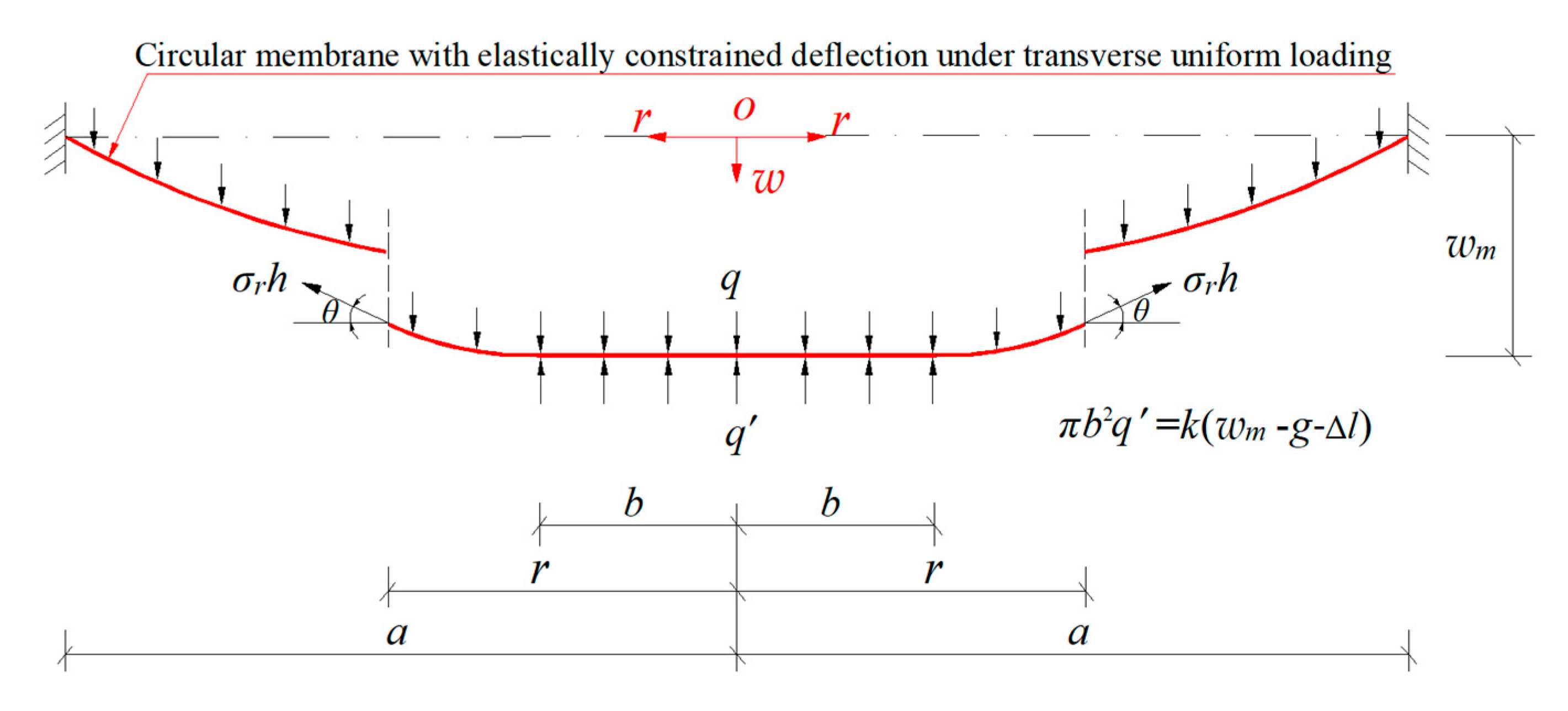
q intensifies, the wind-driven large deflection circular membrane will be in contact elastically with the spring-reset movable electrode plate (its deflection is elastically constrained by the spring-reset movable electrode plate), as shown in
Figure A1b, where the contact radius between the spring-reset movable electrode plate and the wind-driven large deflection circular membrane is denoted by
b. When the interaction between the wind-driven large deflection circular membrane and the spring-reset movable electrode plate reaches static equilibrium, the spring is compressed by Δ
L (Δ
L =
wm −
g, see
Figure A1b) from its original length
L. Such a membrane/plate interaction can be analyzed by introducing a membrane/plate interaction force
q’ that is uniformly distributed over the contact area π
b2, as shown in
Figure A1c, where the upward force perpendicular to the polar plane (
r,
φ) acting on the movable electrode plate is only the restoring force
F (
F =
kΔ
L =
k(
wm −
g)) of the compressed spring, and the downward forces are the external force π
b2 q’ and the self-weight
kΔ
l of the movable electrode plate. So, the static equilibrium condition of the movable electrode plate under the joint actions of π
b2 q’,
kΔ
l and
F is π
b2 q’ +
kΔ
l =
F =
kΔ
L =
k(
wm −
g), as seen in
Figure A1c. This equilibrium condition will be used for analytically solving the large deflection problem of membrane/plate elastic contact in
Figure A1b or
Figure A1c.
Figure A1.
Sketch of the elastic behavior from non-contact to contact between the wind-driven circular membrane and the spring-reset movable electrode plate: (a) the membrane/plate non-contact state; (b) the membrane/plate contact state; (c) a decomposed view of the membrane/plate interaction force.
A free body with a radius
r (
b ≤
r ≤
a) is taken from the central portion of the wind-driven large deflection circular membrane that is being in contact with the spring-reset movable electrode plate, as shown in
Figure A2, where
σr represents the radial stress at
r,
σrh is the membrane force that is acting on the boundary of the radius
r, and
θ denotes the meridional rotation angle of the deflected circular membrane at
r. In the vertical direction perpendicular to the polar plane (
r,
φ), the static equilibrium condition of this free body under the transverse uniform loading of the wind pressure
q is
where 2
πrσrhsin
θ is the vertical component of the radial force acting on the boundary of
r. From the physical phenomenon of the contact problem in
Figure A1, it can be found that
θ = 0 at
r =
b, that is, sin
θ = 0 at
r =
b. Therefore, after applying the condition of sin
θ = 0 at
r =
b to Equation (A1), it can be easily found that
q’ =
q. So, Equation (A1) can be reduced to
where
From Equations (A2) and (A3), the so-called out-of-plane equilibrium equation can be finally written as
Figure A2.
Sketch of the free body with radius r (b ≤ r ≤ a).
Figure A2.
Sketch of the free body with radius r (b ≤ r ≤ a).
In the horizontal direction parallel to the polar plane (
r,
φ), there are only the circumferential stress
σt and the horizontal component of the radial stress
σr. The relationship between radial and circumferential stresses at any point on the circular membrane within the range of
b ≤
r ≤
a, i.e., the in-plane equilibrium equation, is given by [
55]
For large deflection membranes, the so-called geometric equations, that is, the relationships between the radial and circumferential strains,
er and
et, and the radial and transverse displacements,
u and
w, may be written as [
55]
Moreover, for the circular membrane of Hooke-type materials, the physical equations, i.e., the stress and strain relationships, follow Hooke’s law [
55]:
From Equations (A6)–(A9), it is found that
By means of Equations (A10), (A11), and (A5), one has
After substituting the
u of Equation (A12) into Equation (A10), it is found that
Equations (A4) and (A13) are two equations for solving the radial stress σr and transverse displacement w of the membrane/plate non-contact region of b ≤ r ≤ a. With the known solutions of σr and w, the other solutions of σt, er, et, and u can then be easily obtained from Equations (A5), (A6), (A7), and (A12). Therefore, the problem of the membrane/plate non-contact region of b ≤ r ≤ a can be solved analytically.
On the other hand, in the membrane/plate contact region of 0 ≤
r ≤
b, since d
w/d
r = 0, Equations (A6) and (A7) can be reduced to
After substituting d
w/d
r = 0 into Equations (A10) and (A11), it is found that
Substituting Equations (A16) and (A17) into Equation (A5) yields
Since Equation (A18) satisfies the form of the Euler equation, its general solution may be written as
where
C1 and
C2 are two undetermined constants. Obviously, the radial displacement at
r = 0 is equal to zero, i.e.,
u(0) = 0. Since Equation (A19) must satisfy the condition of
u(0) = 0, then
C2 must be identically equal to zero, i.e.,
C2 ≡ 0. If the radial displacement at
r =
b is denoted by
u(
b), then it can be obtained from Equation (A19) that
C1 =
u(
b)/
b, due to
C2 ≡ 0. This results in
If substituting Equation (A20) into Equations (A14)–(A17), then
It can be seen from Equations (A21) and (A22) that in the membrane/plate contact region of 0 ≤
r ≤
b, the strain is uniformly distributed and the radial strain is always equal to the circumferential strain. Also, the stress is uniformly distributed and the radial stress is always equal to the circumferential stress. Note, however, that the contact radius
b and radial displacement
u(
b), like the radial stress
σr and transverse displacement
w of the membrane/plate non-contact region of
b ≤
r ≤
a, are still quantities to be determined at this point.
Obviously, the changes in stress, strain, and displacement in the membrane/plate contact region of 0 ≤
r ≤
b are continuous with those in the membrane/plate non-contact region of
b ≤
r ≤
a. The boundary conditions and continuous conditions, which are used for determining the stress, strain, and displacement of the membrane/plate non-contact region of
b ≤
r ≤
a and the contact radius
b and radial displacement
u(
b) of the membrane/plate contact region of 0 ≤
r ≤
b, are as follows:
where the subscripts
A and
B denote the membrane/plate non-contact and contact regions on the two sides of the inter-connecting circle of
r =
b. In addition, the equilibrium condition of the movable electrode plate under the joint actions of π
b2 q’,
kΔ
l, and
F, that is, π
b2 q’ +
kΔ
l =
k(
wm −
g) (see
Figure A1c), must also be used. This equilibrium condition can be reduced to, from the derivation result
q’ =
q (see the derivation between Equations (A1) and (A2)),
where the maximum membrane deflection
wm is equal to the membrane deflection
w at
r =
b, i.e.,
wm =
w(
b).
Now, let us introduce the following nondimensionalization:
where
b ≤
r ≤
a, i.e.,
α ≤
x ≤ 1. Further, use Equation (A28) to transform Equations (A4) and (A13) and Equations (A23)–(A27) into
where
Wm =
W(
α). Eliminating d
W/d
x from Equations (A29) and (A30) gives
In order to use the power series method for differential equations,
Sr and
W have to be expanded into the power series of
x-
β, where
β = (1 +
α)/2, i.e.,
For convenience, we further introduce
X =
x −
β and reduce Equations (A37) and (A38) to
Also, Equations (A29)–(A36) should be transformed into
After substituting Equation (A39) into Equation (A48), the power series coefficients
ci (
i = 2, 3, 4, …) can be expressed as polynomials with regard to
c0,
c1, and
β (
β = (1 +
α)/2 and
α =
b/
a), which can be seen in
Appendix B, where
c0,
c1, and
β are three undetermined constants. And after substituting Equations (A39) and (A40) into Equation (A42), the power series coefficients
di (
i = 1, 2, 3, …) can also be expressed as polynomials with regard to
c0,
c1, and
β, which can be seen in
Appendix C, where the remaining coefficient
d0 is a dependent undetermined constant (it depends on the undetermined constants
c0,
c1, and
α).
The values of the undetermined coefficients
c0,
c1,
β, and
d0 can be determined by using the above boundary conditions Equations (A43) and (A44), continuous conditions Equations (A45) and (A46), and the equilibrium condition Equation (A47) of the movable electrode plate. Equations (A40), (A43), and (A47) give
Equation (A50) minus Equation (A49) yields
Equations (A39) and (A44)–(A46) give
After eliminating
u(
b)/
b from Equations (A53) and (A54), it is found that
Therefore, for a concrete problem in which the values of a, h, E, v, and q are known beforehand, the undetermined constants c0, c1, and β can be determined by simultaneously solving Equations (A51), (A52), and (A55). Further, with known values for c0, c1, and β, the remaining dependent undetermined constant d0 can be determined by Equation (A49), and the radial displacement u(b) can be determined by Equation (A54). The problem dealt with here is thus solved analytically.
With the known undetermined constants
c0,
c1,
β, and
d0, all the power series coefficients
ci (
i = 2, 3, 4, …,) and
di (
i = 1, 2, 3, …,) can be determined, thus determining all the expressions of
Sr,
St, and
W. Finally, from Equations (A28), (A37), and (A38), the dimensional analytical expressions of
σr and
w can be written as
The maximum membrane deflection
wm is at
r =
b, and thus it is given by the following, from Equation (A57):
In addition, the maximum membrane stress
σm should be in the membrane/plate contact region of 0 ≤
r≤
b. It can be seen from Equations (A21) and (A22) that in the membrane/plate contact region of 0 ≤
r≤
b, the stresses and strains are both uniformly distributed, and the radial stress/strain is always equal to the circumferential stress/strain. Therefore, the maximum membrane stress
σm can be determined by Equation (A22) with the known contact radius
b and radial displacement
u(
b), or given by, from Equation (A56),
The accuracies of the maximum membrane deflection
wm and maximum membrane stress
σm play a very important role in the numerical design and calibration of the parallel plate variable capacitor-based circular wind pressure sensor proposed here.
Appendix D
Table A1.
The numerical calculation results of the undetermined constants β, c0, c1, and d0 as well as maximum stress σm and maximum deflection wm when k = 0.5 N/mm, a = 70 mm, h = 0.3 mm, t = 0.1 mm, E = 3.01 MPa, ν = 0.45, g = 5 mm, Δl = 5 mm, L = 40 mm, and the wind pressure q takes different values.
| q/Pa | β | c0 | c1 | d0 | σm/MPa | wm/mm | C/pF |
|---|
| 164 | 0.508089 | 0.023938 | −0.004382 | 0.109411 | 0.075231 | 10.00132 | 3.8923 |
| 180 | 0.544050 | 0.024999 | −0.004715 | 0.107564 | 0.078310 | 10.0430 | 3.8969 |
| 250 | 0.598700 | 0.029582 | −0.005228 | 0.109212 | 0.091588 | 10.2999 | 3.9257 |
| 450 | 0.649548 | 0.040977 | −0.006322 | 0.119276 | 0.125661 | 11.2394 | 4.0349 |
| 650 | 0.666143 | 0.051272 | −0.007420 | 0.129987 | 0.156822 | 12.2096 | 4.1541 |
| 1000 | 0.675506 | 0.068129 | −0.009289 | 0.147594 | 0.208037 | 13.7933 | 4.3647 |
| 2000 | 0.674910 | 0.112451 | −0.014101 | 0.189765 | 0.342976 | 17.5352 | 4.9585 |
| 3000 | 0.668757 | 0.153851 | −0.018268 | 0.224077 | 0.469091 | 20.5216 | 5.5626 |
| 4000 | 0.662773 | 0.193468 | −0.021953 | 0.253639 | 0.590176 | 23.0514 | 6.2026 |
| 5000 | 0.657493 | 0.232254 | −0.025264 | 0.279991 | 0.707882 | 25.2732 | 6.8999 |
| 6000 | 0.653780 | 0.269163 | −0.028209 | 0.304693 | 0.825293 | 27.3276 | 7.7003 |
| 7000 | 0.649841 | 0.307092 | −0.031039 | 0.326136 | 0.939422 | 29.0912 | 8.5520 |
| 8000 | 0.645980 | 0.344476 | −0.033645 | 0.347378 | 1.051860 | 30.8186 | 9.5910 |
| 9000 | 0.642338 | 0.381389 | −0.036051 | 0.367314 | 1.156710 | 32.4215 | 10.8096 |
| 10000 | 0.639188 | 0.416372 | −0.038191 | 0.385375 | 1.268142 | 33.8582 | 12.1988 |
| 11000 | 0.636385 | 0.452081 | −0.040249 | 0.403105 | 1.375390 | 35.2552 | 13.9410 |
| 12000 | 0.633941 | 0.488016 | −0.042216 | 0.420358 | 1.483440 | 36.6031 | 16.1690 |
| 13000 | 0.631907 | 0.521772 | −0.043989 | 0.436153 | 1.590910 | 37.8286 | 18.9179 |
| 14000 | 0.629948 | 0.557385 | −0.045807 | 0.452525 | 1.697980 | 39.0928 | 22.9413 |
| 15000 | 0.628117 | 0.592392 | −0.047568 | 0.468470 | 1.803200 | 40.3209 | 28.9153 |
Table A2.
The numerical calculation results of the undetermined constants β, c0, c1, and d0 as well as maximum stress σm and maximum deflection wm when k = 0.1 N/mm, a = 70 mm, h = 0.3 mm, t = 0.1 mm, E = 3.01 MPa, ν = 0.45, g = 5 mm, Δl = 5 mm, L = 40 mm, and the wind pressure q takes different values.
| q/Pa | β | c0 | c1 | d0 | σm/MPa | wm/mm | C/pF |
|---|
| 164 | 0.506914 | 0.023946 | −0.004374 | 0.109573 | 0.075252 | 10.00483 | 3.8927 |
| 800 | 0.602296 | 0.065844 | −0.010839 | 0.162026 | 0.203325 | 15.1548 | 4.5635 |
| 1600 | 0.597546 | 0.108481 | −0.016790 | 0.209132 | 0.334643 | 19.3744 | 5.3139 |
| 2400 | 0.591984 | 0.146778 | −0.021637 | 0.244847 | 0.452539 | 22.5038 | 6.0519 |
| 3200 | 0.587431 | 0.182701 | −0.025776 | 0.274563 | 0.563003 | 25.0620 | 6.8270 |
| 4000 | 0.583712 | 0.217076 | −0.029406 | 0.300480 | 0.668585 | 27.2600 | 7.6711 |
| 4800 | 0.580613 | 0.250345 | −0.032648 | 0.323739 | 0.770656 | 29.2067 | 8.6144 |
| 5600 | 0.577964 | 0.282437 | −0.035552 | 0.344809 | 0.869017 | 30.9494 | 9.6800 |
| 6400 | 0.575697 | 0.314539 | −0.038259 | 0.364750 | 0.967315 | 32.5811 | 10.9481 |
| 7200 | 0.573715 | 0.345632 | −0.040715 | 0.383163 | 1.062450 | 34.0728 | 12.4376 |
| 8000 | 0.571922 | 0.376531 | −0.043012 | 0.400710 | 1.156913 | 35.4815 | 14.2712 |
| 8800 | 0.570320 | 0.406999 | −0.045152 | 0.417383 | 1.250000 | 36.8088 | 16.5733 |
| 9600 | 0.568894 | 0.436963 | −0.047137 | 0.433192 | 1.341495 | 38.0567 | 19.5361 |
| 10400 | 0.567597 | 0.466929 | −0.049006 | 0.448450 | 1.432930 | 39.2508 | 23.5677 |
| 11200 | 0.566406 | 0.496490 | −0.050768 | 0.463113 | 1.523100 | 40.3908 | 29.3503 |
Table A3.
The numerical calculation results of the undetermined constants β, c0, c1, and d0 as well as maximum stress σm and maximum deflection wm when k = 1 N/mm, a = 70 mm, h = 0.3 mm, t = 0.1 mm, E = 3.01 MPa, ν = 0.45, g = 5 mm, Δl = 5 mm, L = 40 mm, and the wind pressure q takes different values.
| q/Pa | β | c0 | c1 | d0 | σm/MPa | wm/mm | C/pF |
|---|
| 164 | 0.508286 | 0.023936 | −0.004383 | 0.109384 | 0.075227 | 10.00069 | 3.8922 |
| 1300 | 0.711565 | 0.075547 | −0.009120 | 0.146106 | 0.229843 | 13.5829 | 4.3355 |
| 2600 | 0.712401 | 0.125259 | −0.013597 | 0.187818 | 0.380656 | 17.2226 | 4.9028 |
| 3900 | 0.706387 | 0.172868 | −0.017515 | 0.222950 | 0.525154 | 20.2291 | 5.4970 |
| 5200 | 0.700146 | 0.219350 | −0.021007 | 0.253841 | 0.666239 | 22.8264 | 6.1398 |
| 6500 | 0.694480 | 0.265086 | −0.024166 | 0.281772 | 0.805056 | 25.1381 | 6.8531 |
| 7800 | 0.689450 | 0.310275 | −0.027056 | 0.307505 | 0.942204 | 27.2381 | 7.6616 |
| 9100 | 0.684909 | 0.355158 | −0.029732 | 0.331608 | 1.078420 | 29.1799 | 8.5998 |
| 10400 | 0.680995 | 0.399444 | −0.032206 | 0.354198 | 1.212813 | 30.9785 | 9.7001 |
| 11700 | 0.677361 | 0.444432 | −0.034572 | 0.376153 | 1.349330 | 32.7074 | 11.0602 |
| 13000 | 0.674166 | 0.487414 | −0.036712 | 0.396342 | 1.479763 | 34.2815 | 12.6789 |
| 14300 | 0.671252 | 0.530229 | −0.038741 | 0.415799 | 1.609680 | 35.7850 | 14.7393 |
| 15600 | 0.668504 | 0.574475 | −0.040732 | 0.435253 | 1.743941 | 37.2741 | 17.5666 |
| 16900 | 0.666055 | 0.617610 | −0.042573 | 0.453884 | 1.874752 | 38.6875 | 21.4770 |
| 18200 | 0.663750 | 0.661042 | −0.044355 | 0.471687 | 2.006610 | 40.0263 | 27.2152 |
Table A4.
The numerical calculation results of the undetermined constants β, c0, c1, and d0 as well as maximum stress σm and maximum deflection wm when k = 0.5 N/mm, a = 80 mm, h = 0.3 mm, t = 0.1 mm, E = 3.01 MPa, ν = 0.45, g = 5 mm, Δl = 5 mm, L = 40 mm, and the wind pressure q takes different values.
| q/Pa | β | c0 | c1 | d0 | σm/MPa | wm/mm | C/pF |
|---|
| 96 | 0.503799 | 0.018254 | −0.003345 | 0.096033 | 0.057379 | 10.00022 | 5.0836 |
| 700 | 0.689550 | 0.056414 | −0.007571 | 0.131199 | 0.172069 | 14.0454 | 5.7472 |
| 1400 | 0.687513 | 0.092996 | −0.011650 | 0.169036 | 0.283418 | 17.9179 | 6.5679 |
| 2100 | 0.680619 | 0.127106 | −0.015243 | 0.199852 | 0.387316 | 21.0196 | 7.4160 |
| 2800 | 0.674104 | 0.159795 | −0.018466 | 0.226400 | 0.486893 | 23.6520 | 8.3289 |
| 3500 | 0.668405 | 0.191525 | −0.021395 | 0.250050 | 0.583536 | 25.9660 | 9.3395 |
| 4200 | 0.663445 | 0.222550 | −0.024083 | 0.271581 | 0.678017 | 28.0474 | 10.4837 |
| 4900 | 0.659001 | 0.253292 | −0.026592 | 0.291659 | 0.771615 | 29.9668 | 11.8189 |
| 5600 | 0.655252 | 0.283073 | −0.028888 | 0.310091 | 0.862270 | 31.7111 | 13.3660 |
| 6300 | 0.651754 | 0.313475 | −0.031107 | 0.328048 | 0.954795 | 33.3943 | 15.2983 |
| 7000 | 0.648721 | 0.342126 | −0.033096 | 0.344292 | 1.041976 | 34.9036 | 17.5769 |
| 7700 | 0.645941 | 0.372417 | −0.034996 | 0.359974 | 1.129190 | 36.3493 | 20.5018 |
| 8400 | 0.643347 | 0.400114 | −0.036845 | 0.375443 | 1.218373 | 37.7635 | 24.4880 |
| 9100 | 0.641027 | 0.428760 | −0.038560 | 0.390028 | 1.305490 | 39.0855 | 29.9274 |
| 9800 | 0.638853 | 0.457456 | −0.040213 | 0.404264 | 1.392740 | 40.3676 | 38.1446 |
| 10500 | 0.636795 | 0.485605 | −0.041803 | 0.418045 | 1.478328 | 41.6044 | 51.8883 |
Table A5.
The numerical calculation results of the undetermined constants β, c0, c1, and d0 as well as maximum stress σm and maximum deflection wm when k = 0.5 N/mm, a = 90 mm, h = 0.3 mm, t = 0.1 mm, E = 3.01 MPa, ν = 0.45, g = 5 mm, Δl = 5 mm, L = 40 mm, and the wind pressure q takes different values.
| q/Pa | β | c0 | c1 | d0 | σm/MPa | wm/mm | C/pF |
|---|
| 60 | 0.503156 | 0.014394 | −0.002651 | 0.085357 | 0.045259 | 10.00012 | 6.4340 |
| 450 | 0.700743 | 0.043775 | −0.005850 | 0.113347 | 0.133421 | 13.6916 | 7.1917 |
| 900 | 0.700456 | 0.071449 | −0.008998 | 0.144918 | 0.217609 | 17.3622 | 8.1455 |
| 1350 | 0.694031 | 0.097213 | −0.011839 | 0.170923 | 0.296059 | 20.3467 | 9.1301 |
| 1800 | 0.687614 | 0.121856 | −0.014435 | 0.193427 | 0.371114 | 22.8982 | 10.1824 |
| 2250 | 0.681868 | 0.145726 | −0.016831 | 0.213512 | 0.443824 | 25.1503 | 11.3355 |
| 2700 | 0.676800 | 0.169024 | −0.019061 | 0.231809 | 0.514784 | 27.1811 | 12.6247 |
| 3150 | 0.672223 | 0.192024 | −0.021162 | 0.248836 | 0.584834 | 29.0532 | 14.1034 |
| 3600 | 0.668317 | 0.214361 | −0.023111 | 0.264520 | 0.652853 | 30.7627 | 15.7924 |
| 4050 | 0.664666 | 0.237050 | −0.025005 | 0.279729 | 0.721934 | 32.4068 | 17.8481 |
| 4500 | 0.661475 | 0.258481 | −0.026722 | 0.293520 | 0.787180 | 33.8861 | 20.2159 |
| 4950 | 0.658547 | 0.279835 | −0.028368 | 0.307513 | 0.852174 | 35.2982 | 23.1471 |
| 5400 | 0.655796 | 0.301717 | −0.029986 | 0.319869 | 0.918776 | 36.6828 | 26.9834 |
| 5850 | 0.653334 | 0.323022 | −0.031493 | 0.332162 | 0.983596 | 37.9729 | 31.9113 |
| 6300 | 0.651017 | 0.344377 | −0.032955 | 0.344159 | 1.048570 | 39.2247 | 38.7840 |
| 6750 | 0.648819 | 0.365337 | −0.034365 | 0.355774 | 1.112348 | 40.4330 | 48.9625 |
Table A6.
The numerical calculation results of the undetermined constants β, c0, c1, and d0 as well as maximum stress σm and maximum deflection wm when k = 0.5 N/mm, a = 70 mm, h = 0.1 mm, t = 0.1 mm, E = 3.01 MPa, ν = 0.45, g = 5 mm, Δl = 5 mm, L = 40 mm, and the wind pressure q takes different values.
| q/Pa | β | c0 | c1 | d0 | σm/MPa | wm/mm | C/pF |
|---|
| 54.5 | 0.504683 | 0.023909 | −0.004348 | 0.109770 | 0.075129 | 10.00015 | 3.8922 |
| 500 | 0.732368 | 0.079161 | −0.008883 | 0.143855 | 0.240433 | 13.3247 | 4.3002 |
| 1000 | 0.735016 | 0.131186 | −0.013015 | 0.184199 | 0.397997 | 16.8019 | 4.8298 |
| 1500 | 0.729675 | 0.181754 | −0.016657 | 0.219000 | 0.551757 | 19.7444 | 5.3916 |
| 2000 | 0.723679 | 0.231645 | −0.019927 | 0.250047 | 0.702417 | 22.3230 | 6.0037 |
| 2500 | 0.716990 | 0.279793 | −0.022831 | 0.277421 | 0.848754 | 24.5634 | 6.6607 |
| 3000 | 0.713010 | 0.330253 | −0.025653 | 0.304747 | 1.001299 | 26.7632 | 7.4625 |
| 3500 | 0.708746 | 0.378837 | −0.028191 | 0.329421 | 1.148490 | 28.7249 | 8.3600 |
| 4000 | 0.704376 | 0.427835 | −0.030597 | 0.352975 | 1.297116 | 30.5757 | 9.4299 |
| 4500 | 0.700561 | 0.476959 | −0.032877 | 0.375651 | 1.446090 | 32.4324 | 10.8189 |
| 5000 | 0.697314 | 0.524673 | −0.034982 | 0.396920 | 1.590723 | 33.9729 | 12.3253 |
| 5500 | 0.694342 | 0.571729 | −0.036966 | 0.417242 | 1.733400 | 35.5213 | 14.3309 |
| 6000 | 0.691476 | 0.620256 | −0.038923 | 0.437581 | 1.880550 | 37.0572 | 17.0892 |
| 6500 | 0.688819 | 0.668647 | −0.040792 | 0.457298 | 2.027310 | 38.5329 | 20.9664 |
| 7000 | 0.686385 | 0.716643 | −0.042571 | 0.476358 | 2.172881 | 39.9471 | 26.7918 |
Table A7.
The numerical calculation results of the undetermined constants β, c0, c1, and d0 as well as maximum stress σm and maximum deflection wm when k = 0.5 N/mm, a = 70 mm, h = 0.5 mm, t = 0.1 mm, E = 3.01 MPa, ν = 0.45, g = 5 mm, Δl = 5 mm, L = 40 mm, and the wind pressure q takes different values.
| q/Pa | β | c0 | c1 | d0 | σm/MPa | wm/mm | C/pF |
|---|
| 272 | 0.500873 | 0.023896 | −0.004311 | 0.110235 | 0.075064 | 10.00003 | 3.8921 |
| 1600 | 0.650959 | 0.069444 | −0.010107 | 0.154929 | 0.212687 | 14.4903 | 4.4643 |
| 3200 | 0.647272 | 0.115047 | −0.015574 | 0.198540 | 0.352011 | 18.4655 | 5.1321 |
| 4800 | 0.640592 | 0.157020 | −0.020196 | 0.236404 | 0.480293 | 21.6843 | 5.8395 |
| 6400 | 0.634700 | 0.196961 | −0.024222 | 0.266922 | 0.602320 | 24.3005 | 6.5763 |
| 8000 | 0.629711 | 0.235558 | −0.027849 | 0.293877 | 0.720184 | 26.5760 | 7.3868 |
| 9600 | 0.625830 | 0.274003 | −0.031096 | 0.319211 | 0.837682 | 28.6803 | 8.3372 |
| 11200 | 0.622372 | 0.311102 | −0.034047 | 0.341872 | 0.950778 | 30.5440 | 9.4093 |
| 12800 | 0.618950 | 0.345548 | −0.036603 | 0.361610 | 1.061940 | 32.1508 | 10.5825 |
| 14400 | 0.615850 | 0.381522 | −0.039106 | 0.381203 | 1.171510 | 33.7294 | 12.0599 |
| 16000 | 0.613148 | 0.417107 | −0.041442 | 0.399901 | 1.273850 | 35.2211 | 13.8926 |
| 17600 | 0.610823 | 0.452363 | −0.043631 | 0.417891 | 1.381160 | 36.6431 | 16.2461 |
| 19200 | 0.608781 | 0.487299 | −0.045680 | 0.435156 | 1.487460 | 37.9953 | 19.3658 |
| 20800 | 0.606930 | 0.521925 | −0.047596 | 0.451683 | 1.592850 | 39.2782 | 23.6799 |
| 22400 | 0.605195 | 0.556306 | −0.049407 | 0.467611 | 1.697530 | 40.5057 | 30.0945 |
Table A8.
The numerical calculation results of the undetermined constants β, c0, c1, and d0 as well as maximum stress σm and maximum deflection wm when k = 0.5 N/mm, a = 70 mm, h = 0.3 mm, t = 2.5 mm, E = 3.01 MPa, ν = 0.45, g = 5 mm, Δl = 5 mm, L = 40 mm, and the wind pressure q takes different values.
| q/Pa | β | c0 | c1 | d0 | σm/MPa | wm/mm | C/pF |
|---|
| 164 | 0.508089 | 0.023938 | −0.004382 | 0.109411 | 0.075231 | 10.00132 | 3.7959 |
| 180 | 0.544050 | 0.024999 | −0.004715 | 0.107564 | 0.078310 | 10.0430 | 3.8003 |
| 250 | 0.598700 | 0.029582 | −0.005228 | 0.109212 | 0.091588 | 10.2999 | 3.8277 |
| 450 | 0.649548 | 0.040977 | −0.006322 | 0.119276 | 0.125661 | 11.2394 | 3.9314 |
| 650 | 0.666143 | 0.051272 | −0.007420 | 0.129987 | 0.156822 | 12.2096 | 4.0445 |
| 1000 | 0.675506 | 0.068129 | −0.009289 | 0.147594 | 0.208037 | 13.7933 | 4.2439 |
| 2000 | 0.674910 | 0.112451 | −0.014101 | 0.189765 | 0.342976 | 17.5352 | 4.8032 |
| 3000 | 0.668757 | 0.153851 | −0.018268 | 0.224077 | 0.469091 | 20.5216 | 5.3678 |
| 4000 | 0.662773 | 0.193468 | −0.021953 | 0.253639 | 0.590176 | 23.0514 | 5.9615 |
| 5000 | 0.657493 | 0.232254 | −0.025264 | 0.279991 | 0.707882 | 25.2732 | 6.6028 |
| 6000 | 0.653780 | 0.269163 | −0.028209 | 0.304693 | 0.825293 | 27.3276 | 7.3321 |
| 7000 | 0.649841 | 0.307092 | −0.031039 | 0.326136 | 0.939422 | 29.0912 | 8.1002 |
| 8000 | 0.645980 | 0.344476 | −0.033645 | 0.347378 | 1.051860 | 30.8186 | 9.0264 |
| 9000 | 0.642338 | 0.381389 | −0.036051 | 0.367314 | 1.156710 | 32.4215 | 10.0977 |
| 10000 | 0.639188 | 0.416372 | −0.038191 | 0.385375 | 1.268142 | 33.8582 | 11.2998 |
| 11000 | 0.636385 | 0.452081 | −0.040249 | 0.403105 | 1.375390 | 35.2552 | 12.7791 |
| 12000 | 0.633941 | 0.488016 | −0.042216 | 0.420358 | 1.483440 | 36.6031 | 14.6267 |
| 13000 | 0.631907 | 0.521772 | −0.043989 | 0.436153 | 1.590910 | 37.8286 | 16.8402 |
| 14000 | 0.629948 | 0.557385 | −0.045807 | 0.452525 | 1.697980 | 39.0928 | 19.9556 |
| 15000 | 0.628117 | 0.592392 | −0.047568 | 0.468470 | 1.803200 | 40.3209 | 24.3276 |
Table A9.
The numerical calculation results of the undetermined constants β, c0, c1, and d0 as well as maximum stress σm and maximum deflection wm when k = 0.5 N/mm, a = 70 mm, h = 0.3 mm, t = 5 mm, E = 3.01 MPa, ν = 0.45, g = 5 mm, Δl = 5 mm, L = 40 mm, and the wind pressure q takes different values.
| q/Pa | β | c0 | c1 | d0 | σm/MPa | wm/mm | C/pF |
|---|
| 164 | 0.508089 | 0.023938 | −0.004382 | 0.109411 | 0.075231 | 10.00132 | 3.7005 |
| 180 | 0.544050 | 0.024999 | −0.004715 | 0.107564 | 0.078310 | 10.0430 | 3.7047 |
| 250 | 0.598700 | 0.029582 | −0.005228 | 0.109212 | 0.091588 | 10.2999 | 3.7307 |
| 450 | 0.649548 | 0.040977 | −0.006322 | 0.119276 | 0.125661 | 11.2394 | 3.8291 |
| 650 | 0.666143 | 0.051272 | −0.007420 | 0.129987 | 0.156822 | 12.2096 | 3.9364 |
| 1000 | 0.675506 | 0.068129 | −0.009289 | 0.147594 | 0.208037 | 13.7933 | 4.1250 |
| 2000 | 0.674910 | 0.112451 | −0.014101 | 0.189765 | 0.342976 | 17.5352 | 4.6514 |
| 3000 | 0.668757 | 0.153851 | −0.018268 | 0.224077 | 0.469091 | 20.5216 | 5.1790 |
| 4000 | 0.662773 | 0.193468 | −0.021953 | 0.253639 | 0.590176 | 23.0514 | 5.7294 |
| 5000 | 0.657493 | 0.232254 | −0.025264 | 0.279991 | 0.707882 | 25.2732 | 6.3193 |
| 6000 | 0.653780 | 0.269163 | −0.028209 | 0.304693 | 0.825293 | 27.3276 | 6.9842 |
| 7000 | 0.649841 | 0.307092 | −0.031039 | 0.326136 | 0.939422 | 29.0912 | 7.6777 |
| 8000 | 0.645980 | 0.344476 | −0.033645 | 0.347378 | 1.051860 | 30.8186 | 8.5049 |
| 9000 | 0.642338 | 0.381389 | −0.036051 | 0.367314 | 1.156710 | 32.4215 | 9.4495 |
| 10000 | 0.639188 | 0.416372 | −0.038191 | 0.385375 | 1.268142 | 33.8582 | 10.4943 |
| 11000 | 0.636385 | 0.452081 | −0.040249 | 0.403105 | 1.375390 | 35.2552 | 11.7583 |
| 12000 | 0.633941 | 0.488016 | −0.042216 | 0.420358 | 1.483440 | 36.6031 | 13.3046 |
| 13000 | 0.631907 | 0.521772 | −0.043989 | 0.436153 | 1.590910 | 37.8286 | 15.1114 |
| 14000 | 0.629948 | 0.557385 | −0.045807 | 0.452525 | 1.697980 | 39.0928 | 17.5732 |
| 15000 | 0.628117 | 0.592392 | −0.047568 | 0.468470 | 1.803200 | 40.3209 | 20.8773 |
Table A10.
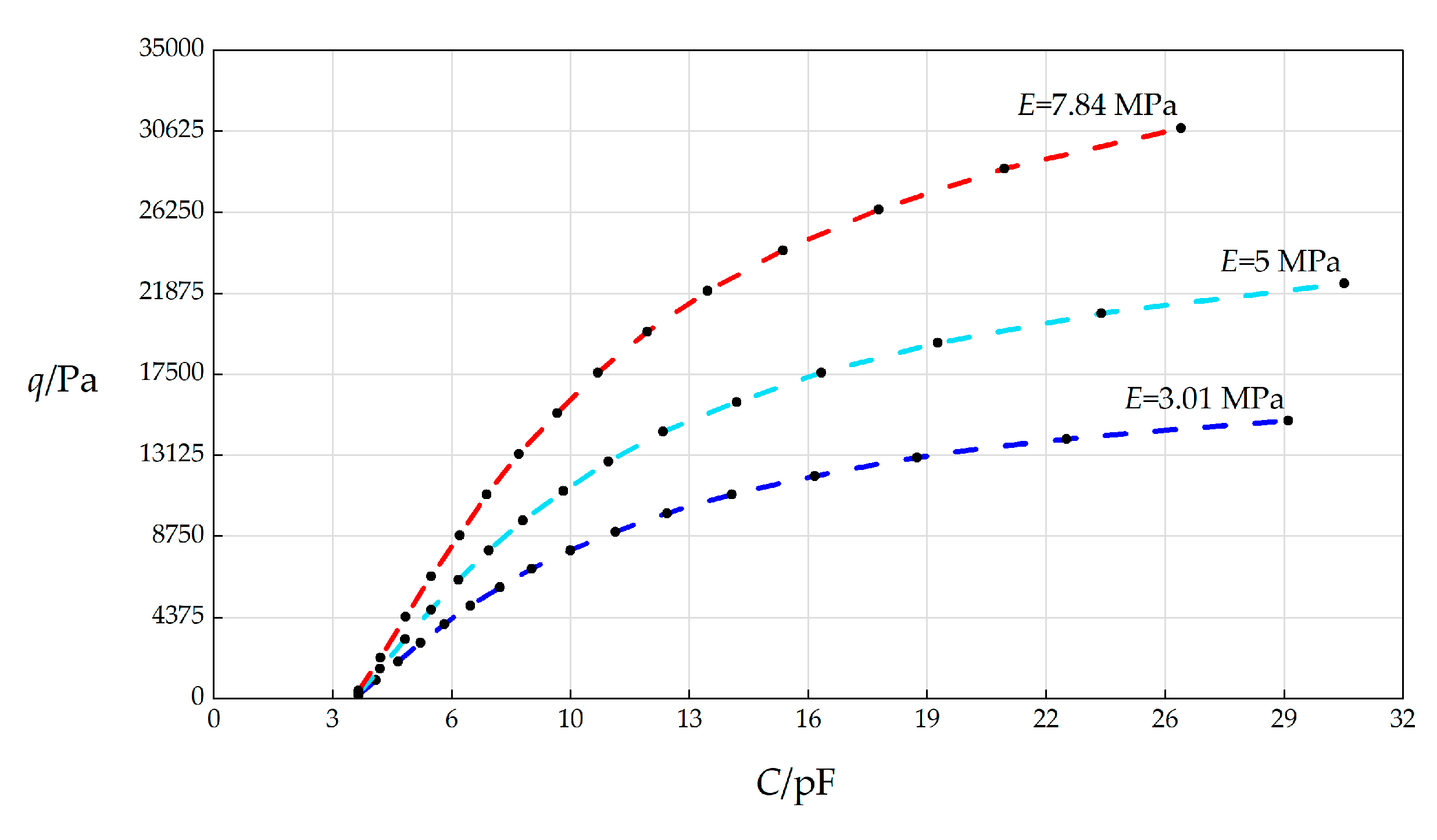
The numerical calculation results of the undetermined constants β, c0, c1, and d0 as well as maximum stress σm and maximum deflection wm when k = 0.5 N/mm, a = 70 mm, h = 0.3 mm, t = 0.1 mm, E = 5 MPa, ν = 0.45, g = 5 mm, Δl = 5 mm, L = 40 mm, and the wind pressure q takes different values.
Table A10.
The numerical calculation results of the undetermined constants β, c0, c1, and d0 as well as maximum stress σm and maximum deflection wm when k = 0.5 N/mm, a = 70 mm, h = 0.3 mm, t = 0.1 mm, E = 5 MPa, ν = 0.45, g = 5 mm, Δl = 5 mm, L = 40 mm, and the wind pressure q takes different values.
| q/Pa | β | c0 | c1 | d0 | σm/MPa | wm/mm | C/pF |
|---|
| 272 | 0.506278 | 0.023924 | −0.004365 | 0.109603 | 0.124889 | 10.00132 | 3.8923 |
| 1600 | 0.651132 | 0.069586 | −0.010120 | 0.155046 | 0.354013 | 14.5006 | 4.4658 |
| 3200 | 0.647404 | 0.115300 | −0.015596 | 0.200633 | 0.586010 | 18.5626 | 5.1510 |
| 4800 | 0.640709 | 0.157381 | −0.020224 | 0.236633 | 0.799644 | 21.7036 | 5.8444 |
| 6400 | 0.634806 | 0.197428 | −0.024255 | 0.267195 | 1.002880 | 24.3231 | 6.5834 |
| 8000 | 0.629020 | 0.236678 | −0.027884 | 0.294250 | 1.202070 | 26.6096 | 7.4003 |
| 9600 | 0.625553 | 0.273860 | −0.031062 | 0.319114 | 1.390482 | 28.6365 | 8.3149 |
| 11200 | 0.621988 | 0.311804 | −0.034075 | 0.340597 | 1.582810 | 30.5410 | 9.4073 |
| 12800 | 0.618661 | 0.347240 | −0.036700 | 0.362150 | 1.762241 | 32.1954 | 10.6193 |
| 14400 | 0.615616 | 0.382484 | −0.039152 | 0.382598 | 1.940730 | 33.7548 | 12.0870 |
| 16000 | 0.613236 | 0.418187 | −0.041615 | 0.401429 | 2.121400 | 35.3408 | 14.0641 |
| 17600 | 0.610975 | 0.453787 | −0.043676 | 0.418558 | 2.301466 | 36.6933 | 16.3438 |
| 19200 | 0.608904 | 0.488583 | −0.045842 | 0.435712 | 2.477470 | 38.0371 | 19.4814 |
| 20800 | 0.606978 | 0.523341 | −0.047662 | 0.452295 | 2.653190 | 39.3255 | 23.8760 |
| 22400 | 0.605232 | 0.557826 | −0.049476 | 0.468252 | 2.827480 | 40.5548 | 30.4242 |
Table A11.
The numerical calculation results of the undetermined constants β, c0, c1, and d0 as well as maximum stress σm and maximum deflection wm when k = 0.5 N/mm, a = 70 mm, h = 0.3 mm, t = 0.1 mm, E = 7.84 MPa, ν = 0.45, g = 5 mm, Δl = 5 mm, L = 40 mm, and the wind pressure q takes different values.
| q/Pa | β | c0 | c1 | d0 | σm/MPa | wm/mm | C/pF |
|---|
| 425.5 | 0.503027 | 0.023904 | −0.004332 | 0.109969 | 0.195615 | 10.00048 | 3.8922 |
| 2200 | 0.629902 | 0.065748 | −0.010172 | 0.155656 | 0.526224 | 14.5719 | 4.4762 |
| 4400 | 0.626162 | 0.108487 | −0.015720 | 0.200883 | 0.867405 | 18.6248 | 5.1631 |
| 6600 | 0.620013 | 0.147354 | −0.020357 | 0.236029 | 1.177759 | 21.7067 | 5.8451 |
| 8800 | 0.616775 | 0.185102 | −0.024487 | 0.267615 | 1.462990 | 24.4164 | 6.6132 |
| 11000 | 0.610230 | 0.219360 | −0.027927 | 0.291563 | 1.752221 | 26.4598 | 7.3406 |
| 13200 | 0.606452 | 0.253633 | −0.031122 | 0.314971 | 2.025360 | 28.4212 | 8.2072 |
| 15400 | 0.603421 | 0.286574 | −0.033982 | 0.336210 | 2.287700 | 30.2740 | 9.2372 |
| 17600 | 0.600372 | 0.320005 | −0.036692 | 0.356434 | 2.553775 | 31.8362 | 10.3303 |
| 19800 | 0.597814 | 0.352086 | −0.039132 | 0.374988 | 2.808960 | 33.3409 | 11.6593 |
| 22000 | 0.595601 | 0.384164 | −0.041430 | 0.392831 | 3.063970 | 34.7744 | 13.2879 |
| 24200 | 0.593635 | 0.415905 | −0.043579 | 0.409848 | 3.316183 | 36.1295 | 15.3094 |
| 26400 | 0.591816 | 0.447284 | −0.045595 | 0.426102 | 3.565410 | 37.4137 | 17.8883 |
| 28600 | 0.590153 | 0.478166 | −0.047473 | 0.441568 | 3.810578 | 38.6259 | 21.2706 |
| 30800 | 0.588624 | 0.509222 | −0.049262 | 0.456646 | 4.057020 | 39.7981 | 26.0298 |
Table A12.
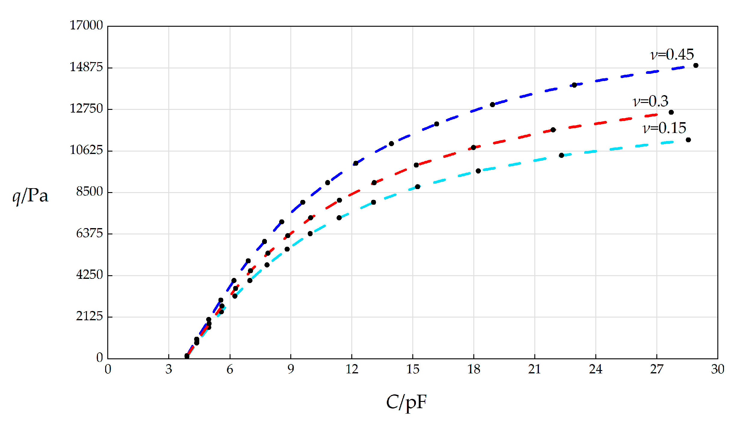
The numerical calculation results of the undetermined constants β, c0, c1, and d0 as well as maximum stress σm and maximum deflection wm when k = 0.5 N/mm, a = 70 mm, h = 0.3 mm, t = 0.1 mm, E = 3.01 MPa, ν = 0.15, g = 5 mm, Δl = 5 mm, L = 40 mm, and the wind pressure q takes different values.
Table A12.
The numerical calculation results of the undetermined constants β, c0, c1, and d0 as well as maximum stress σm and maximum deflection wm when k = 0.5 N/mm, a = 70 mm, h = 0.3 mm, t = 0.1 mm, E = 3.01 MPa, ν = 0.15, g = 5 mm, Δl = 5 mm, L = 40 mm, and the wind pressure q takes different values.
| q/Pa | β | c0 | c1 | d0 | σm/MPa | wm/mm | C/pF |
|---|
| 114 | 0.502118 | 0.017071 | −0.004091 | 0.111054 | 0.054335 | 10.00006 | 3.8921 |
| 800 | 0.696036 | 0.050333 | −0.009000 | 0.148883 | 0.154106 | 13.7861 | 4.3637 |
| 1600 | 0.695694 | 0.083397 | −0.013576 | 0.191910 | 0.254962 | 17.5459 | 4.9605 |
| 2400 | 0.689363 | 0.114742 | −0.017549 | 0.227568 | 0.350638 | 20.5983 | 5.5800 |
| 3200 | 0.683099 | 0.145103 | −0.021077 | 0.258646 | 0.443319 | 23.2117 | 6.2482 |
| 4000 | 0.676066 | 0.174679 | −0.024248 | 0.286202 | 0.533598 | 25.4956 | 6.9784 |
| 4800 | 0.672640 | 0.203992 | −0.027167 | 0.312231 | 0.623050 | 27.6181 | 7.8288 |
| 5600 | 0.668516 | 0.233131 | −0.029878 | 0.336452 | 0.711961 | 29.5698 | 8.8166 |
| 6400 | 0.664515 | 0.261286 | −0.032336 | 0.358562 | 0.797859 | 31.3318 | 9.9501 |
| 7200 | 0.660951 | 0.290251 | −0.034721 | 0.380394 | 0.886219 | 33.0526 | 11.3788 |
| 8000 | 0.658013 | 0.317497 | −0.036847 | 0.400205 | 0.969318 | 34.5988 | 13.0643 |
| 8800 | 0.655111 | 0.344901 | −0.038884 | 0.419481 | 1.052890 | 36.0901 | 15.2419 |
| 9600 | 0.652655 | 0.372902 | −0.040861 | 0.438531 | 1.138277 | 37.5505 | 18.2152 |
| 10400 | 0.650328 | 0.400352 | −0.042700 | 0.456624 | 1.221970 | 38.9247 | 22.3104 |
| 11200 | 0.648163 | 0.427854 | −0.044472 | 0.474342 | 1.305820 | 40.2608 | 28.5514 |
Table A13.
The numerical calculation results of the undetermined constants β, c0, c1, and d0 as well as maximum stress σm and maximum deflection wm when k = 0.5 N/mm, a = 70 mm, h = 0.3 mm, t = 0.1 mm, E = 3.01 MPa, ν = 0.3, g = 5 mm, Δl = 5 mm, L = 40 mm, and the wind pressure q takes different values.
| q/Pa | β | c0 | c1 | d0 | σm/MPa | wm/mm | C/pF |
|---|
| 133.5 | 0.502762 | 0.019770 | −0.004206 | 0.110515 | 0.062554 | 10.00013 | 3.8922 |
| 900 | 0.687098 | 0.058331 | −0.009240 | 0.149294 | 0.178366 | 13.8799 | 4.3768 |
| 1800 | 0.686150 | 0.096640 | −0.014001 | 0.192514 | 0.295120 | 17.6813 | 4.9850 |
| 2700 | 0.679709 | 0.132723 | −0.018120 | 0.227982 | 0.405157 | 20.7384 | 5.6122 |
| 3600 | 0.673471 | 0.167542 | −0.021766 | 0.258715 | 0.511337 | 23.3412 | 6.2855 |
| 4500 | 0.667132 | 0.201523 | −0.025047 | 0.285957 | 0.614946 | 25.6157 | 7.0216 |
| 5400 | 0.663170 | 0.234853 | −0.028031 | 0.311402 | 0.716535 | 27.7057 | 7.8683 |
| 6300 | 0.659129 | 0.268199 | −0.030816 | 0.335195 | 0.818157 | 29.6372 | 8.8552 |
| 7200 | 0.655226 | 0.300167 | −0.033318 | 0.356708 | 0.915562 | 31.3648 | 9.9741 |
| 8100 | 0.651690 | 0.33323 | −0.035754 | 0.378028 | 1.016280 | 33.0586 | 11.3845 |
| 9000 | 0.648877 | 0.365298 | −0.037984 | 0.397942 | 1.108540 | 34.6246 | 13.0967 |
| 9900 | 0.646172 | 0.395755 | −0.039996 | 0.416227 | 1.206697 | 36.0496 | 15.1733 |
| 10800 | 0.643710 | 0.426985 | −0.041964 | 0.434404 | 1.301780 | 37.4549 | 17.9855 |
| 11700 | 0.641407 | 0.458348 | −0.043843 | 0.452102 | 1.397261 | 38.8114 | 21.9044 |
| 12600 | 0.639304 | 0.489624 | −0.045625 | 0.469250 | 1.492460 | 40.1146 | 27.7034 |
Table A14.
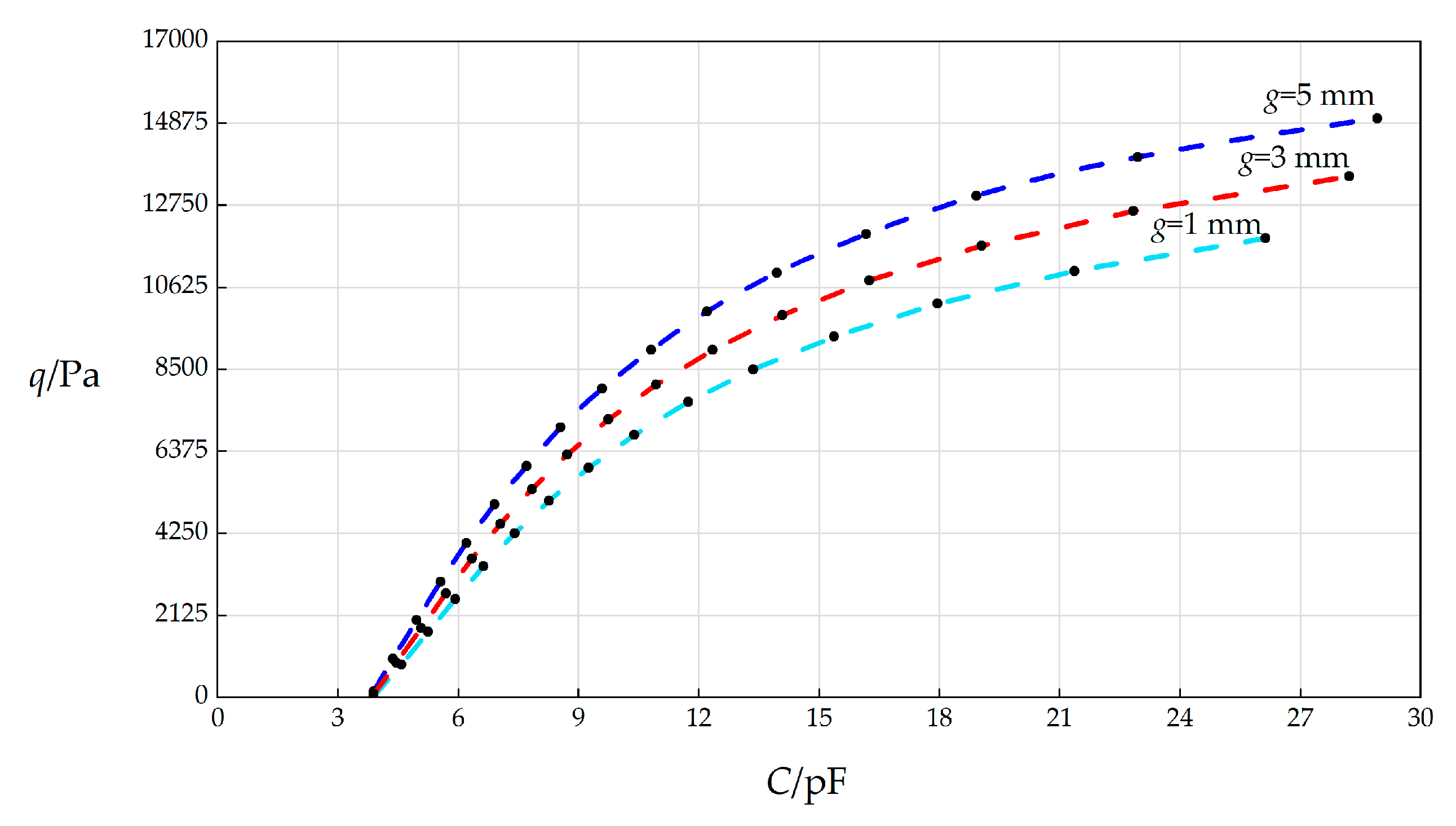
The numerical calculation results of the undetermined constants β, c0, c1, and d0 as well as maximum stress σm and maximum deflection wm when k = 0.5 N/mm, a = 70 mm, h = 0.3 mm, t = 0.1 mm, E = 3.01 MPa, ν = 0.45, g = 1 mm, Δl = 5 mm, L = 40 mm, and the wind pressure q takes different values.
Table A14.
The numerical calculation results of the undetermined constants β, c0, c1, and d0 as well as maximum stress σm and maximum deflection wm when k = 0.5 N/mm, a = 70 mm, h = 0.3 mm, t = 0.1 mm, E = 3.01 MPa, ν = 0.45, g = 1 mm, Δl = 5 mm, L = 40 mm, and the wind pressure q takes different values.
| q/Pa | β | c0 | c1 | d0 | σm/MPa | wm/mm | C/pF |
|---|
| 35.6 | 0.507215 | 0.008550 | −0.001603 | 0.065493 | 0.026904 | 6.00023 | 3.8922 |
| 850 | 0.724312 | 0.053934 | −0.006581 | 0.120561 | 0.164006 | 11.2669 | 4.5807 |
| 1700 | 0.708062 | 0.092562 | −0.010893 | 0.162745 | 0.281578 | 15.0630 | 5.2502 |
| 2550 | 0.695527 | 0.128630 | −0.014666 | 0.196068 | 0.391411 | 18.0058 | 5.9210 |
| 3400 | 0.685891 | 0.163203 | −0.018040 | 0.224411 | 0.496698 | 20.4687 | 6.6300 |
| 4250 | 0.678180 | 0.196765 | −0.021100 | 0.249483 | 0.598896 | 22.6166 | 7.4031 |
| 5100 | 0.671805 | 0.229586 | −0.023904 | 0.272209 | 0.698823 | 24.5386 | 8.2656 |
| 5950 | 0.666403 | 0.261833 | −0.026494 | 0.293152 | 0.796988 | 26.2896 | 9.2469 |
| 6800 | 0.661735 | 0.293621 | −0.028903 | 0.312689 | 0.893734 | 27.9056 | 10.3849 |
| 7650 | 0.657642 | 0.325028 | −0.031156 | 0.331081 | 0.989303 | 29.4120 | 11.7306 |
| 8500 | 0.654006 | 0.356114 | −0.033271 | 0.348522 | 1.083876 | 30.8274 | 13.3569 |
| 9350 | 0.650745 | 0.386922 | −0.035266 | 0.365158 | 1.177589 | 32.1659 | 15.3722 |
| 10200 | 0.647795 | 0.417487 | −0.037154 | 0.381102 | 1.270550 | 33.4384 | 17.9465 |
| 11050 | 0.645107 | 0.447839 | −0.038947 | 0.396444 | 1.362843 | 34.6534 | 21.3622 |
| 11900 | 0.642643 | 0.477998 | −0.040653 | 0.411257 | 1.454539 | 35.8182 | 26.1300 |
Table A15.
The numerical calculation results of the undetermined constants β, c0, c1, and d0 as well as maximum stress σm and maximum deflection wm when k = 0.5 N/mm, a = 70 mm, h = 0.3 mm, t = 0.1 mm, E = 3.01 MPa, ν = 0.45, g = 3 mm, Δl = 5 mm, L = 40 mm, and the wind pressure q takes different values.
| q/Pa | β | c0 | c1 | d0 | σm/MPa | wm/mm | C/pF |
|---|
| 84.3 | 0.508782 | 0.015260 | −0.002837 | 0.087317 | 0.047992 | 8.00080 | 3.8922 |
| 900 | 0.699680 | 0.059863 | −0.007746 | 0.132820 | 0.182392 | 12.4192 | 4.4539 |
| 1800 | 0.691609 | 0.100386 | −0.012240 | 0.174406 | 0.305766 | 16.1385 | 5.0698 |
| 2700 | 0.682432 | 0.138220 | −0.016151 | 0.207762 | 0.421005 | 19.0663 | 5.6890 |
| 3600 | 0.674713 | 0.174507 | −0.019633 | 0.236324 | 0.531534 | 21.5328 | 6.3415 |
| 4500 | 0.668274 | 0.209756 | −0.022779 | 0.261691 | 0.638880 | 23.6921 | 7.0493 |
| 5400 | 0.662819 | 0.244244 | −0.025653 | 0.284747 | 0.743890 | 25.6294 | 7.8339 |
| 6300 | 0.658120 | 0.278145 | −0.028301 | 0.306040 | 0.847089 | 27.3977 | 8.7196 |
| 7200 | 0.654013 | 0.311575 | −0.030758 | 0.325936 | 0.948830 | 29.0322 | 9.7373 |
| 8100 | 0.650379 | 0.344616 | −0.033051 | 0.344693 | 1.049364 | 30.5579 | 10.9277 |
| 9000 | 0.647131 | 0.377326 | −0.035202 | 0.362502 | 1.148873 | 31.9930 | 12.3477 |
| 9900 | 0.644200 | 0.409752 | −0.037227 | 0.379507 | 1.247498 | 33.3514 | 14.0795 |
| 10800 | 0.641537 | 0.441929 | −0.039140 | 0.395820 | 1.345349 | 34.6440 | 16.2478 |
| 11700 | 0.639101 | 0.473886 | −0.040955 | 0.411532 | 1.442513 | 35.8793 | 19.0519 |
| 12600 | 0.636860 | 0.505646 | −0.042681 | 0.426714 | 1.539062 | 37.0644 | 22.8322 |
| 13500 | 0.634789 | 0.537227 | −0.044326 | 0.441426 | 1.635056 | 38.2048 | 28.2206 |
Table A16.
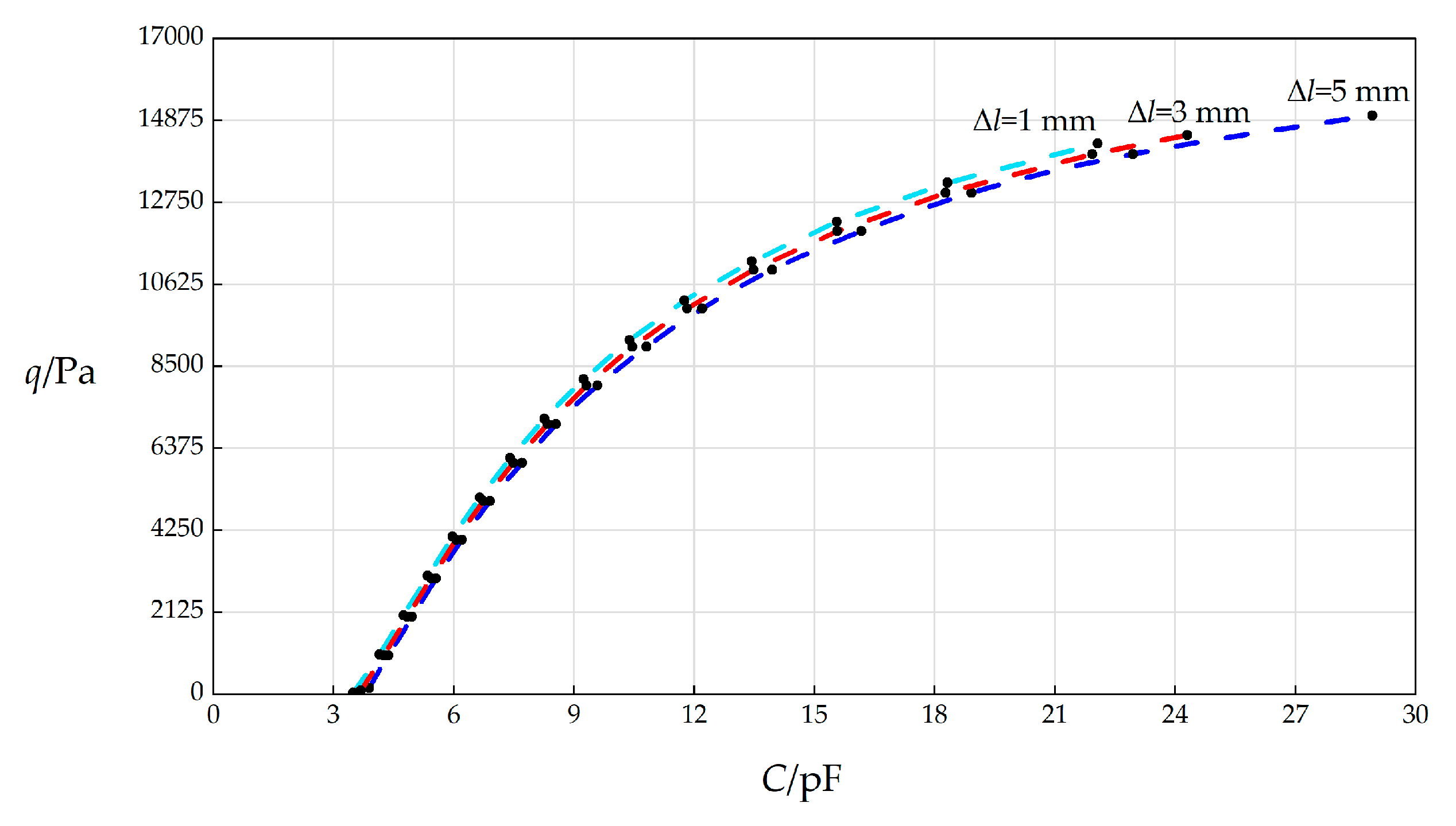
The numerical calculation results of the undetermined constants β, c0, c1, and d0 as well as maximum stress σm and maximum deflection wm when k = 0.5 N/mm, a = 70 mm, h = 0.3 mm, t = 0.1 mm, E = 3.01 MPa, ν = 0.45, g = 5 mm, Δl = 1 mm, L = 40 mm, and the wind pressure q takes different values.
Table A16.
The numerical calculation results of the undetermined constants β, c0, c1, and d0 as well as maximum stress σm and maximum deflection wm when k = 0.5 N/mm, a = 70 mm, h = 0.3 mm, t = 0.1 mm, E = 3.01 MPa, ν = 0.45, g = 5 mm, Δl = 1 mm, L = 40 mm, and the wind pressure q takes different values.
| q/Pa | β | c0 | c1 | d0 | σm/MPa | wm/mm | C/pF |
|---|
| 35.5 | 0.503347 | 0.008542 | −0.001590 | 0.065756 | 0.026872 | 6.00005 | 3.4933 |
| 1020 | 0.720888 | 0.061962 | −0.007496 | 0.130066 | 0.188433 | 12.1288 | 4.1439 |
| 2040 | 0.702618 | 0.107215 | −0.012458 | 0.176841 | 0.326198 | 16.3139 | 4.7477 |
| 3060 | 0.689470 | 0.149516 | −0.016732 | 0.213537 | 0.455015 | 19.5282 | 5.3459 |
| 4080 | 0.679600 | 0.190118 | −0.020510 | 0.244680 | 0.578659 | 22.2073 | 5.9733 |
| 5100 | 0.671805 | 0.229586 | −0.023904 | 0.272209 | 0.698823 | 24.5386 | 6.6526 |
| 6120 | 0.665416 | 0.268225 | −0.026990 | 0.297162 | 0.816442 | 26.6227 | 7.4056 |
| 7140 | 0.660036 | 0.306226 | −0.029822 | 0.320171 | 0.932091 | 28.5202 | 8.2564 |
| 8160 | 0.655411 | 0.343715 | −0.032440 | 0.341650 | 1.046157 | 30.2712 | 9.2354 |
| 9180 | 0.651371 | 0.380781 | −0.034876 | 0.361890 | 1.158910 | 31.9038 | 10.3835 |
| 10200 | 0.647795 | 0.417487 | −0.037154 | 0.381102 | 1.270550 | 33.4384 | 11.7573 |
| 11220 | 0.644598 | 0.453885 | −0.039294 | 0.399446 | 1.381228 | 34.8902 | 13.4395 |
| 12240 | 0.641712 | 0.490012 | −0.041313 | 0.417047 | 1.491063 | 36.2713 | 15.5570 |
| 13260 | 0.639089 | 0.525898 | −0.043223 | 0.434003 | 1.600150 | 37.5910 | 18.3143 |
| 14280 | 0.636688 | 0.561570 | −0.045036 | 0.450393 | 1.708566 | 38.8569 | 22.0656 |
| 15300 | 0.634479 | 0.597047 | −0.046763 | 0.466282 | 1.816376 | 40.0753 | 27.4840 |
Table A17.
The numerical calculation results of the undetermined constants β, c0, c1, and d0 as well as maximum stress σm and maximum deflection wm when k = 0.5 N/mm, a = 70 mm, h = 0.3 mm, t = 0.1 mm, E = 3.01 MPa, ν = 0.45, g = 5 mm, Δl = 3 mm, L = 40 mm, and the wind pressure q takes different values.
| q/Pa | β | c0 | c1 | d0 | σm/MPa | wm/mm | C/pF |
|---|
| 84 | 0.504741 | 0.015240 | −0.002812 | 0.087662 | 0.047920 | 8.00023 | 3.6820 |
| 1000 | 0.699278 | 0.064572 | −0.008281 | 0.138046 | 0.196719 | 12.8905 | 4.2421 |
| 2000 | 0.689464 | 0.108968 | −0.013153 | 0.182361 | 0.331905 | 16.8413 | 4.8365 |
| 3000 | 0.679697 | 0.150455 | −0.017354 | 0.217714 | 0.458275 | 19.9300 | 5.4315 |
| 4000 | 0.671712 | 0.190282 | −0.021068 | 0.247929 | 0.579576 | 22.5243 | 6.0574 |
| 5000 | 0.665138 | 0.228997 | −0.024406 | 0.274744 | 0.697468 | 24.7919 | 6.7359 |
| 6000 | 0.659613 | 0.266902 | −0.027441 | 0.299113 | 0.812866 | 26.8246 | 7.4877 |
| 7000 | 0.654881 | 0.304183 | −0.030227 | 0.321621 | 0.926333 | 28.6791 | 8.3366 |
| 8000 | 0.650763 | 0.340962 | −0.032804 | 0.342659 | 1.038247 | 30.3931 | 9.3123 |
| 9000 | 0.647131 | 0.377326 | −0.035202 | 0.362502 | 1.148873 | 31.9930 | 10.4545 |
| 10000 | 0.643892 | 0.413339 | −0.037444 | 0.381352 | 1.258407 | 33.4981 | 11.8181 |
| 11000 | 0.640977 | 0.449049 | −0.039552 | 0.399361 | 1.366998 | 34.9232 | 13.4834 |
| 12000 | 0.638334 | 0.484494 | −0.041540 | 0.416648 | 1.474761 | 36.2796 | 15.5718 |
| 13000 | 0.635920 | 0.519703 | −0.043421 | 0.433307 | 1.581792 | 37.5764 | 18.2784 |
| 14000 | 0.633703 | 0.554702 | −0.045208 | 0.449416 | 1.688164 | 38.8209 | 21.9378 |
| 14500 | 0.632660 | 0.572128 | −0.046068 | 0.457283 | 1.741123 | 39.4254 | 24.3011 |


