
Let’s Go Bananas: Beyond Bounding Box Representations for Fisheye Camera-Based Object Detection in Autonomous Driving †


Abstract
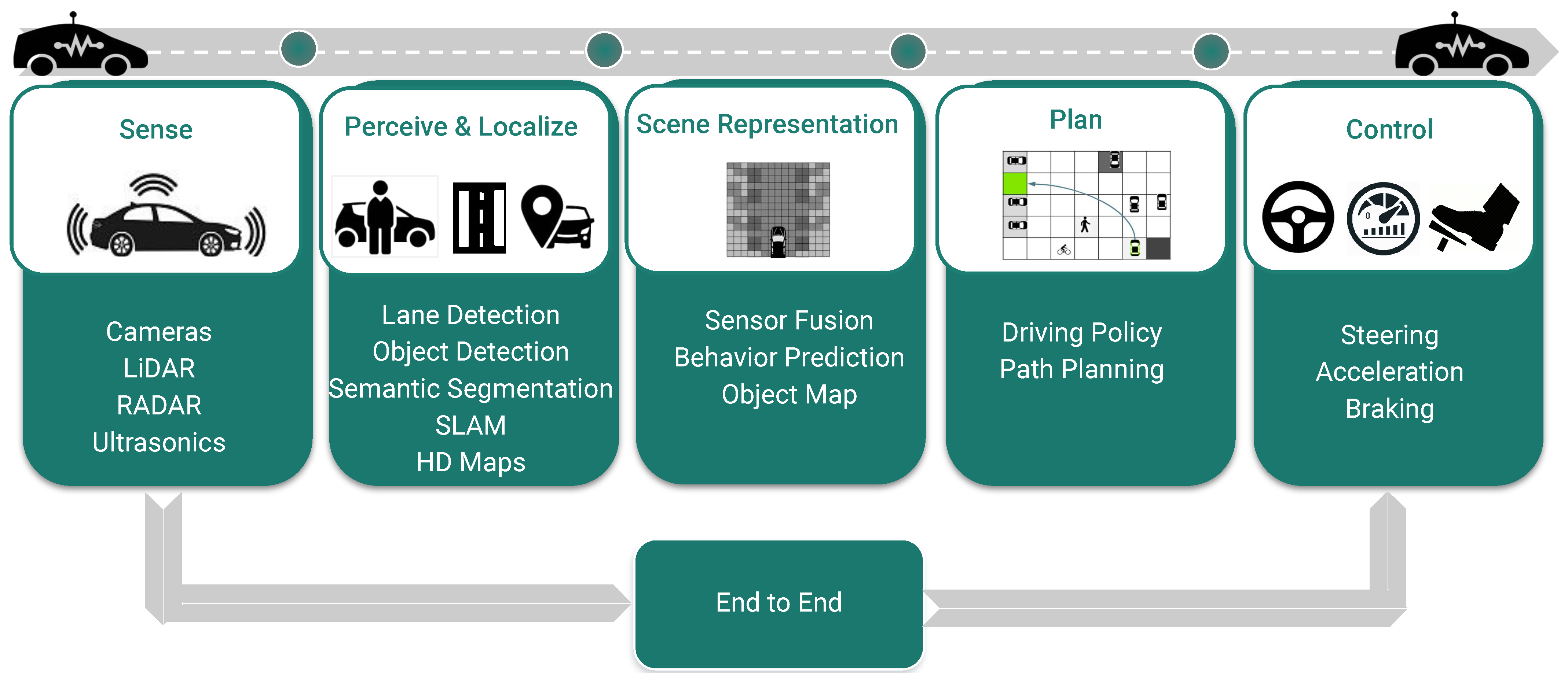
1. Introduction
- Implementation of an extensible YOLO-based framework facilitating comparison of various object representations for fisheye object detection.
- Design of novel representations for fisheye images, including the curved bounding box, vanishing point-based curved bounding box, and adaptive step polygon.
- Design of novel camera tensor representation of radial distortion to enable adaptation of the model to specific camera distortions.
- Ablation study of effect of undistortion, encoder type and temporal models.
2. Related Work
2.1. Object Detection
2.1.1. Two Stage Object Detection
2.1.2. Single Stage Object Detection
2.2. Instance Segmentation
2.2.1. Two Stage Instance Segmentation
2.2.2. Single Stage Instance Segmentation
2.2.3. Polygon Instance Segmentation
2.3. Object Detection on Fisheye Cameras
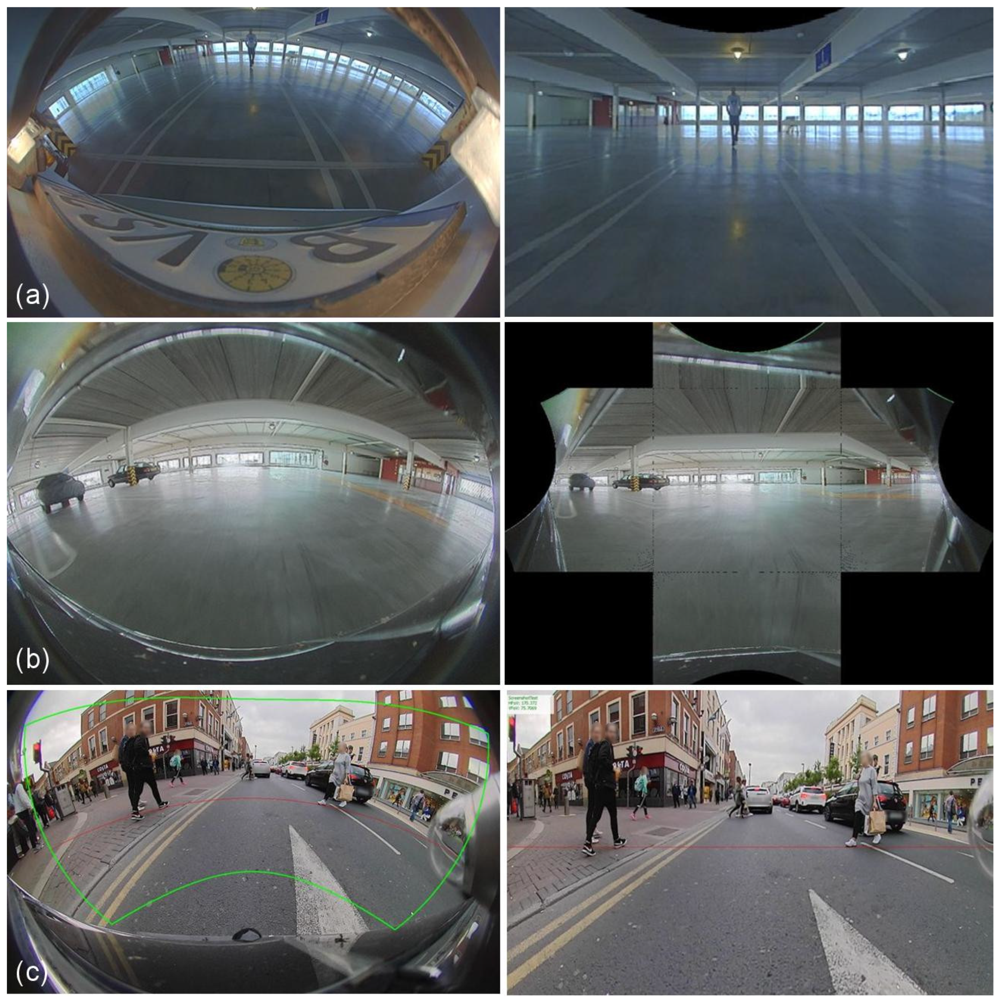
3. Challenges in Object Detection on Fisheye Cameras
3.1. Bounding Boxes on Fisheye
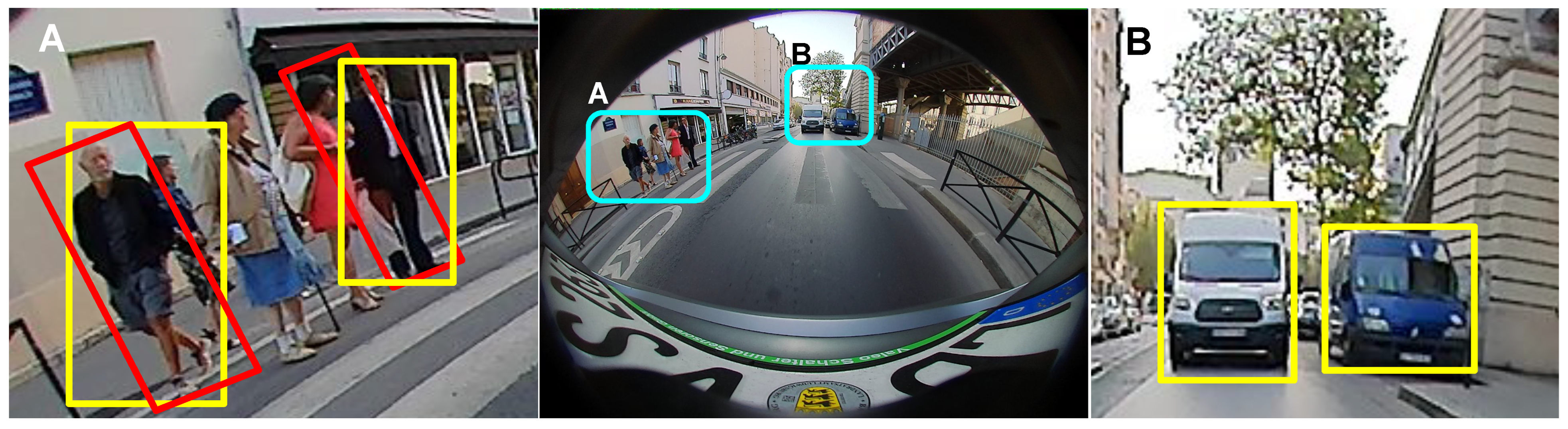
3.1.1. Pedestrian Localization Issue
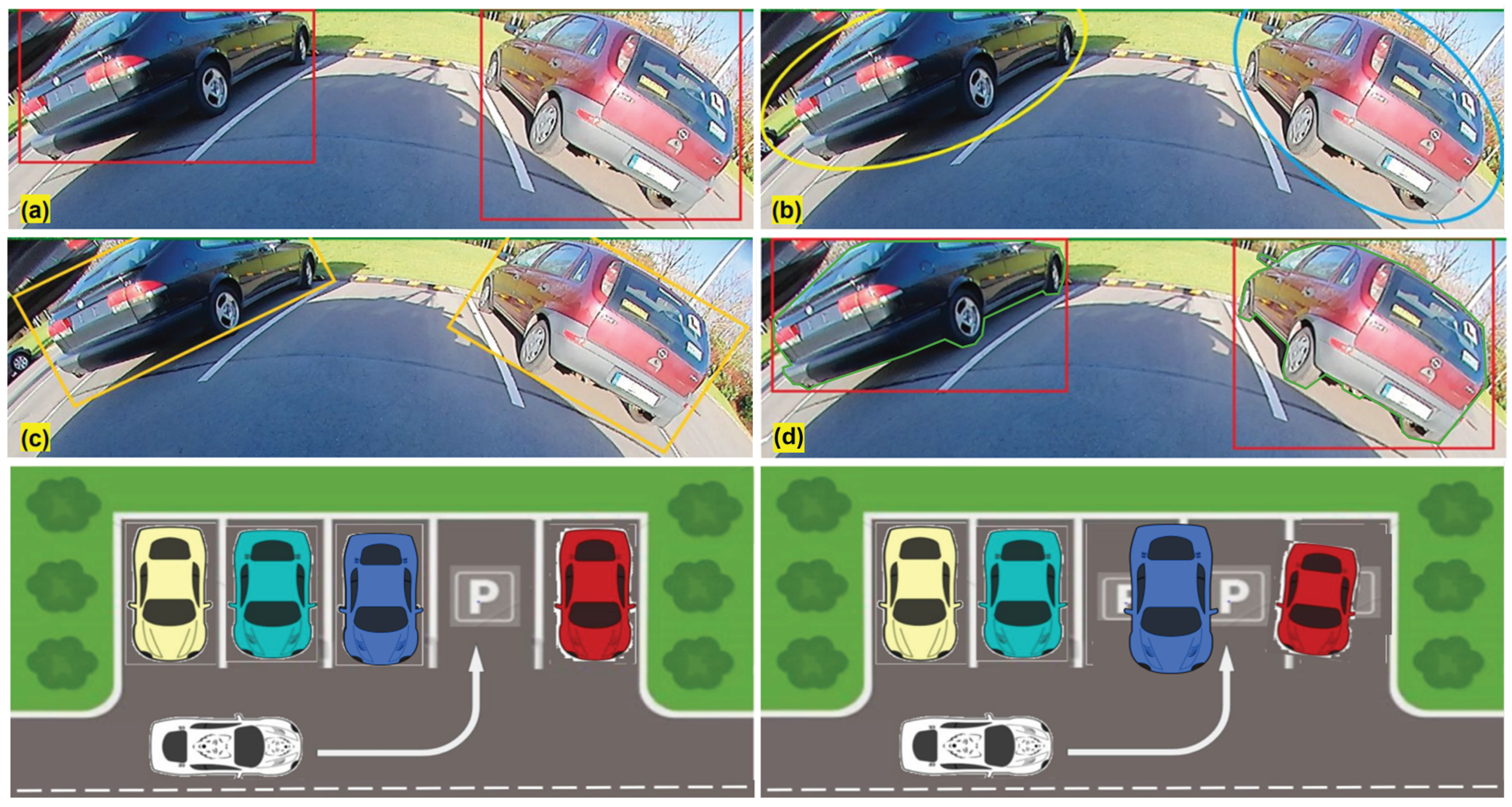
3.1.2. Missing Parking Spot
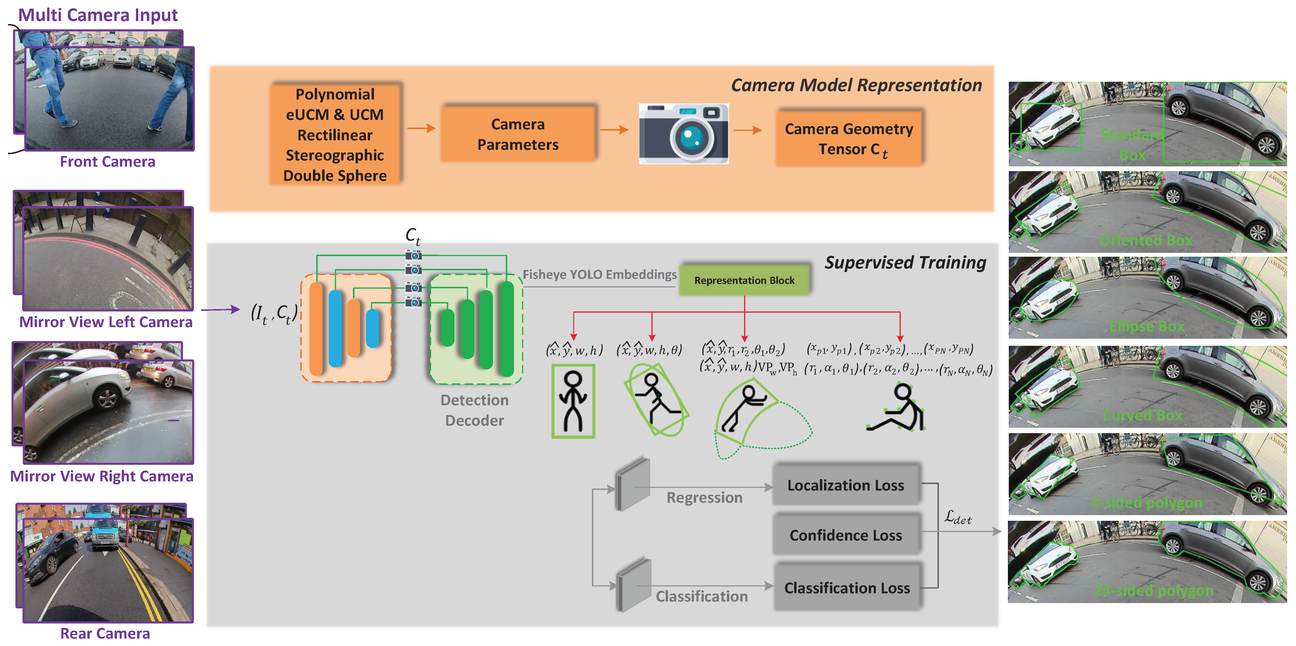
4. Proposed Method
4.1. High Level Architecture
Camera Geometry Tensor
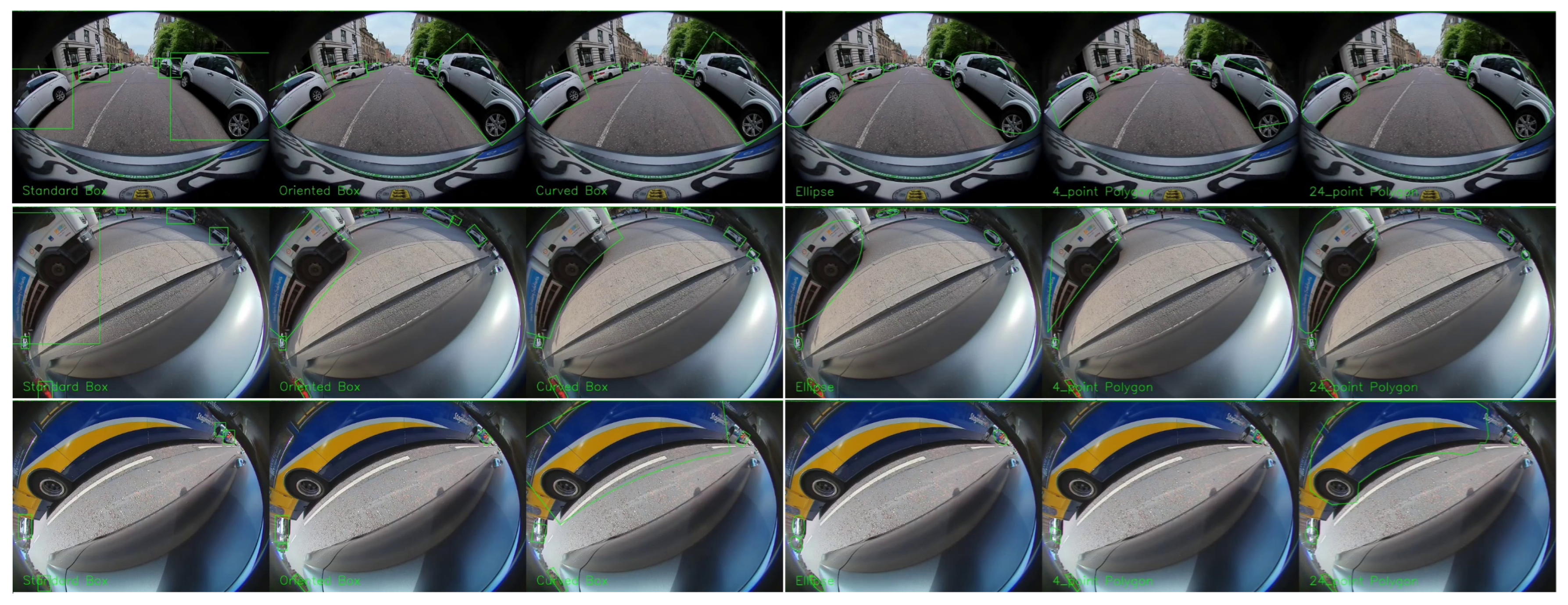
4.2. Basic Object Representations
4.2.1. Bounding Box
4.2.2. Oriented Bounding Box
4.2.3. Ellipse Detection
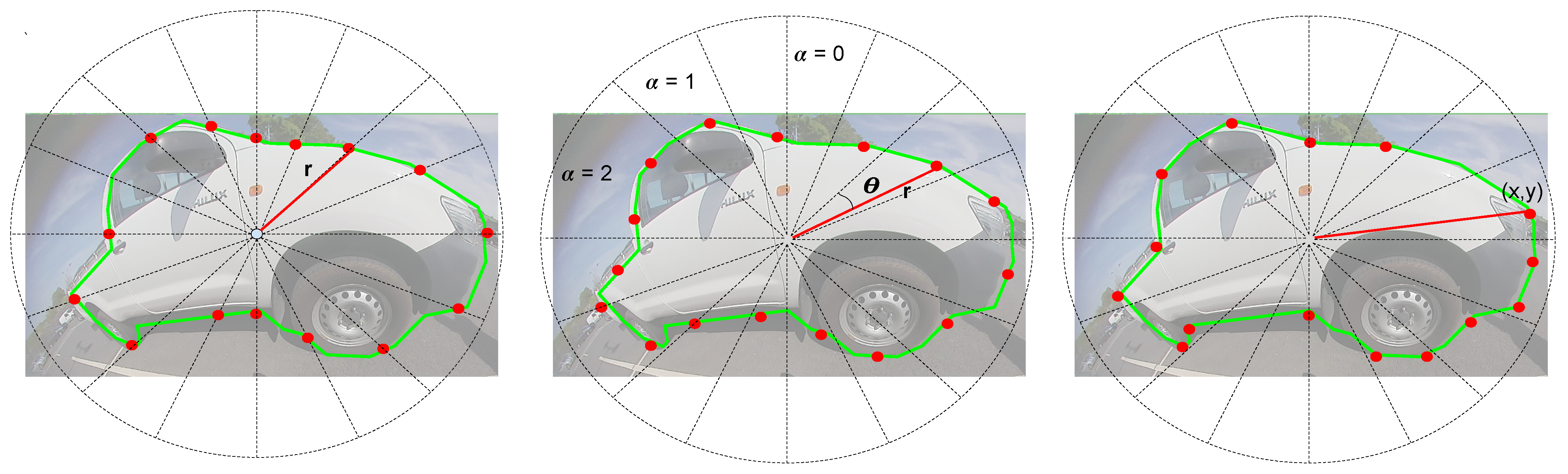
4.3. Generic Polygon Representations
4.4. Distortion Aware Representation
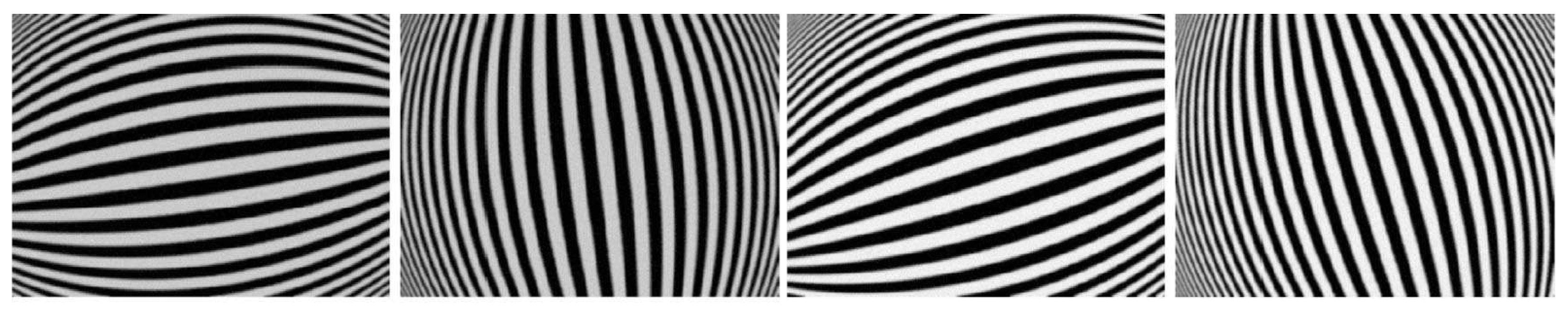
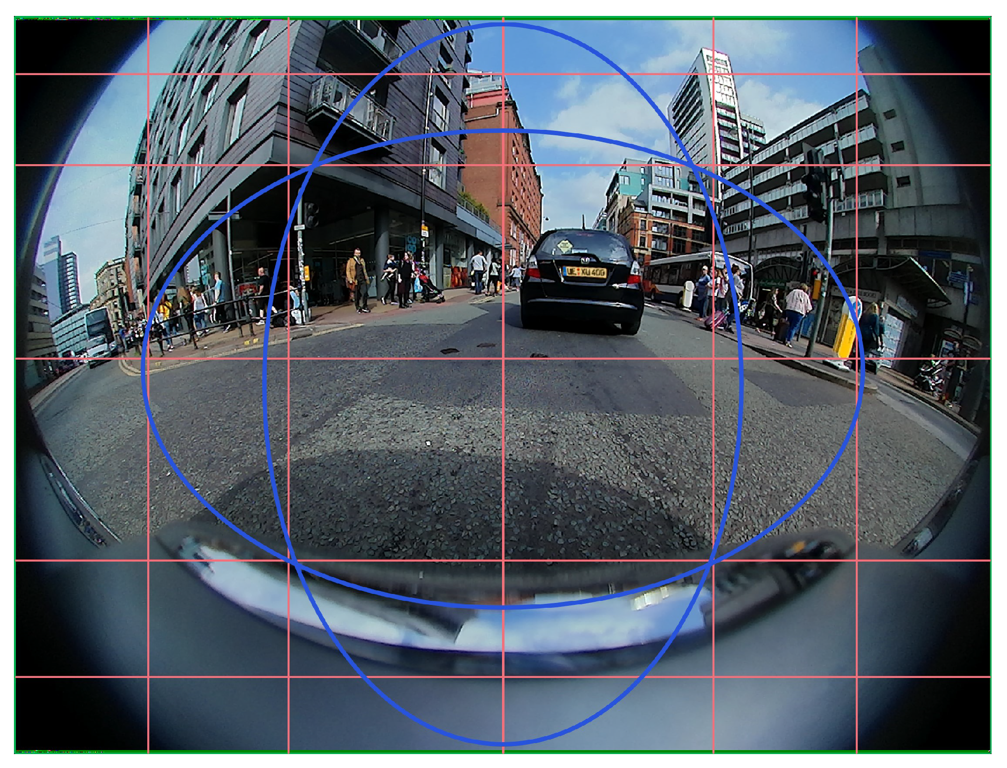
4.4.1. Banana Shaped Curvature in Fisheye Camera Projection
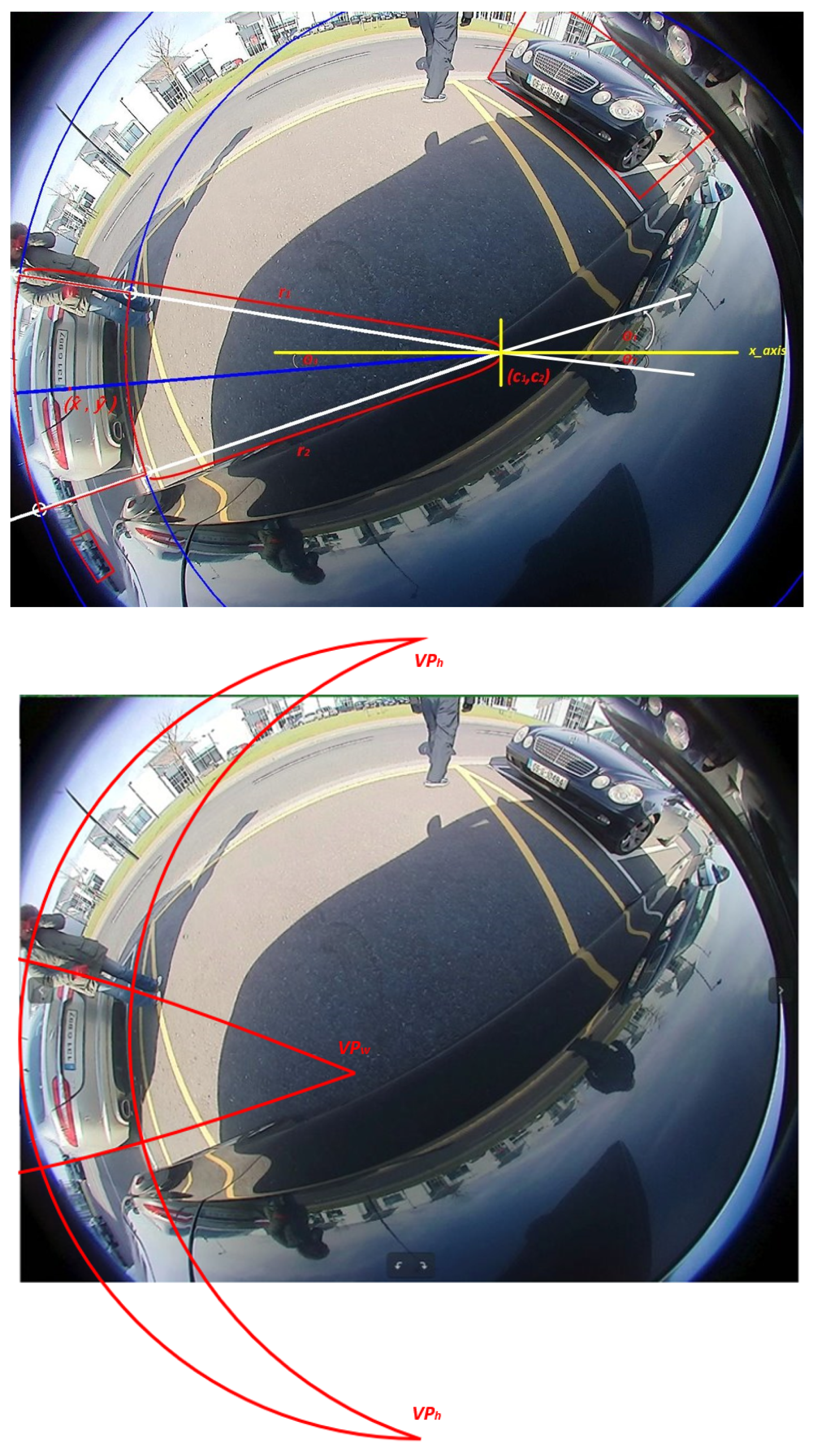
4.4.2. Curved Bounding Box
4.4.3. Vanishing Point Guided Curved Box
5. Experiments
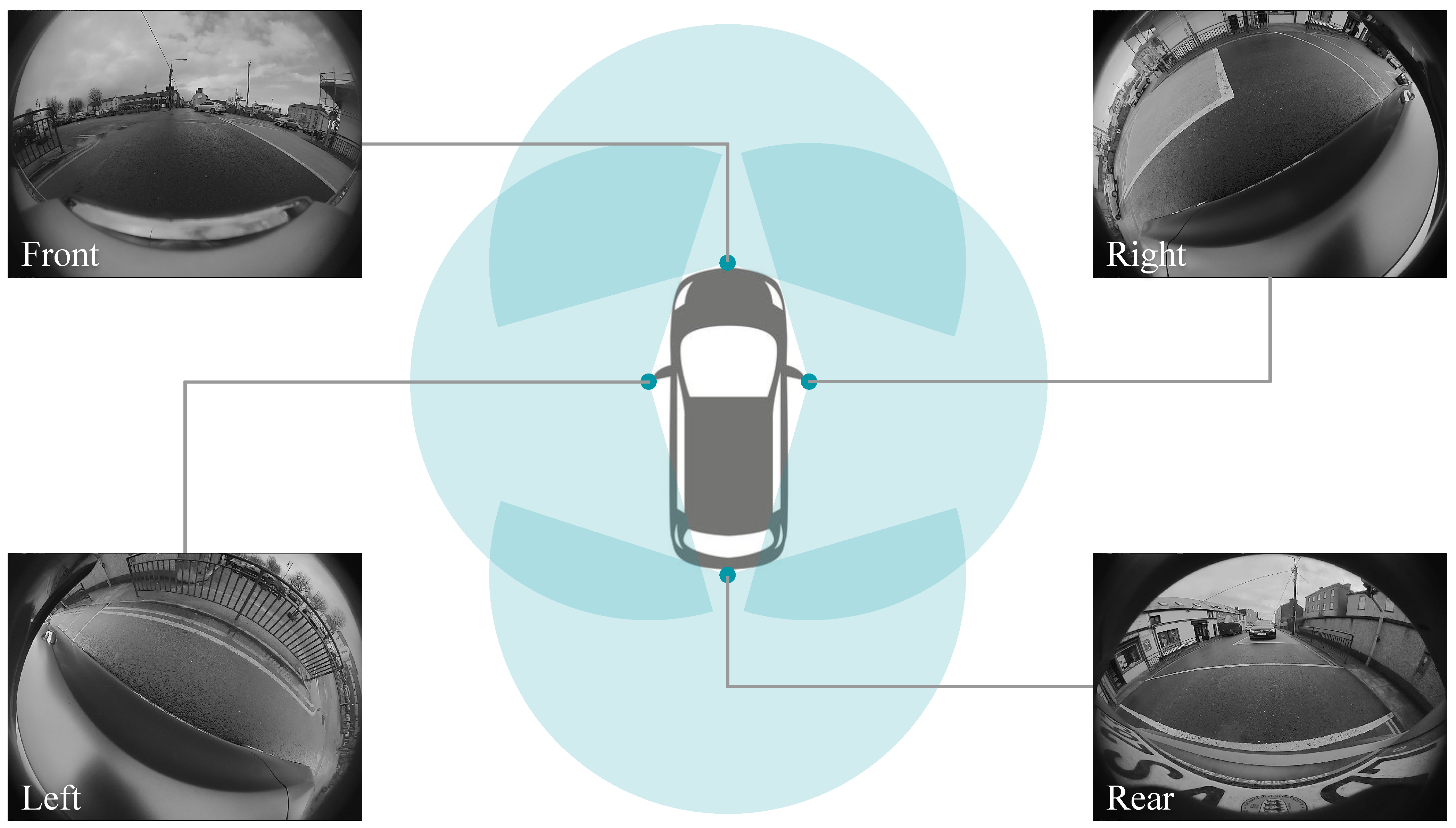
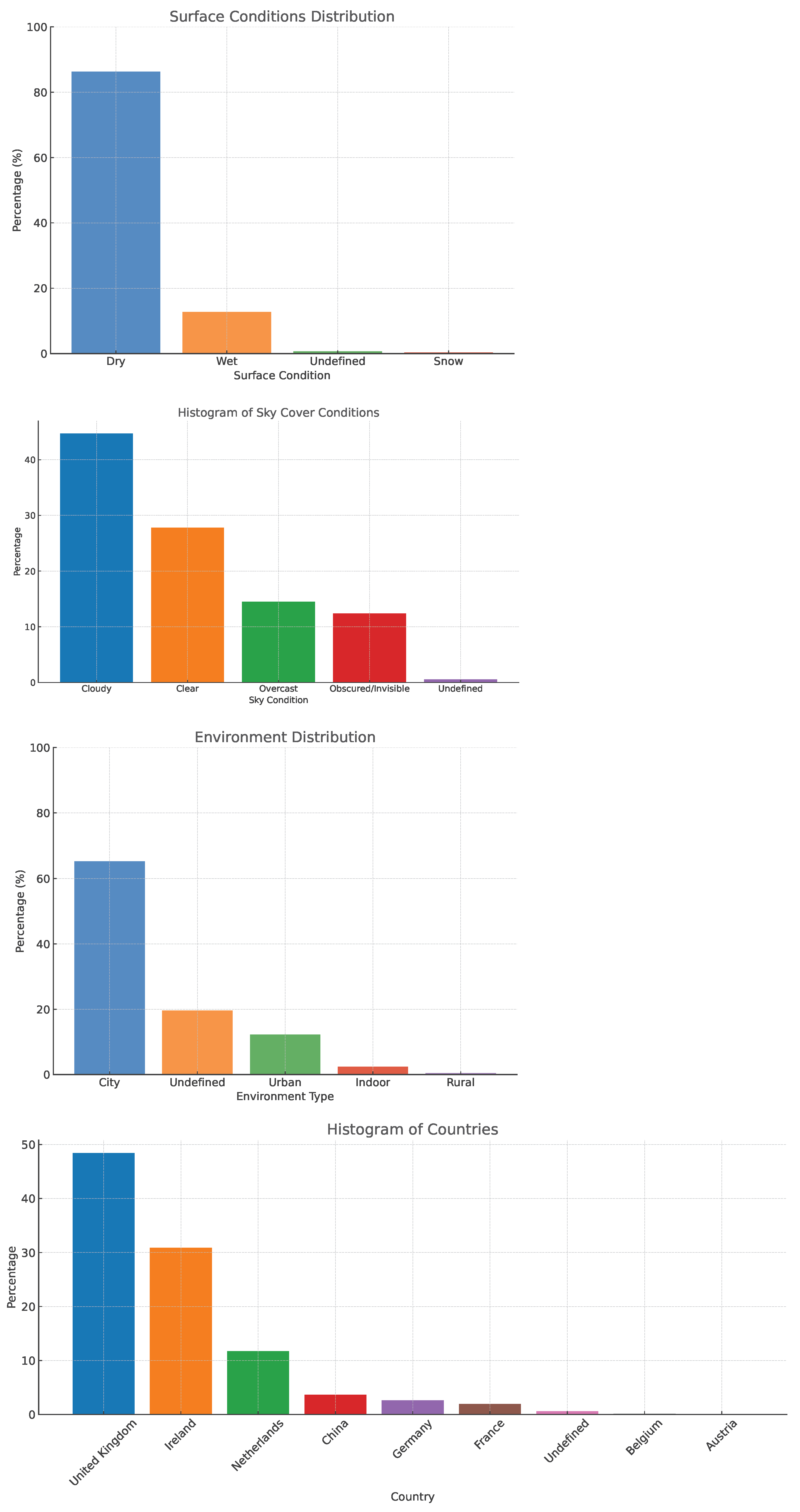
5.1. Dataset and Evaluation Metrics
5.2. Training Details
5.3. Results
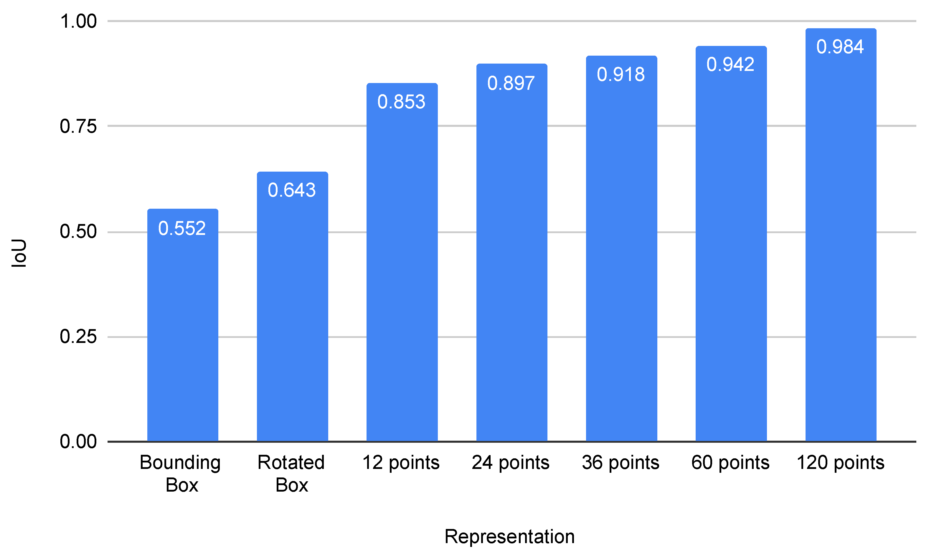
5.3.1. Finding Optimal Number of Polygon Vertices
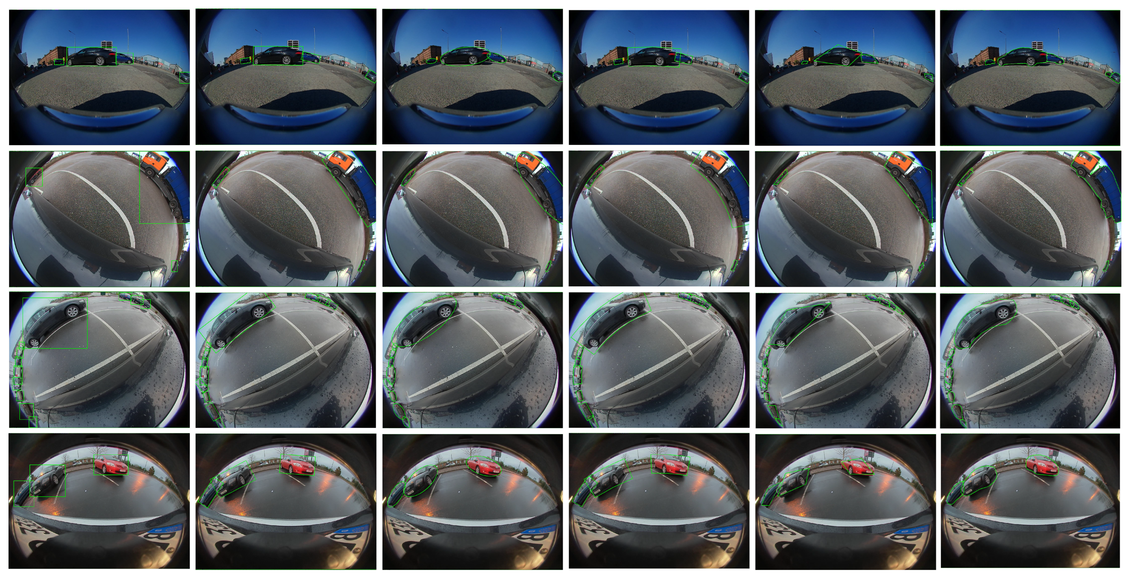
5.3.2. Evaluation of Representation Capacity
5.3.3. Standardized Evaluation Using Segmentation Masks
5.3.4. Real-World Application Related Metrics
5.3.5. Ablation Study
5.3.6. Quantitative Results on Proposed Curved Bounding Boxes
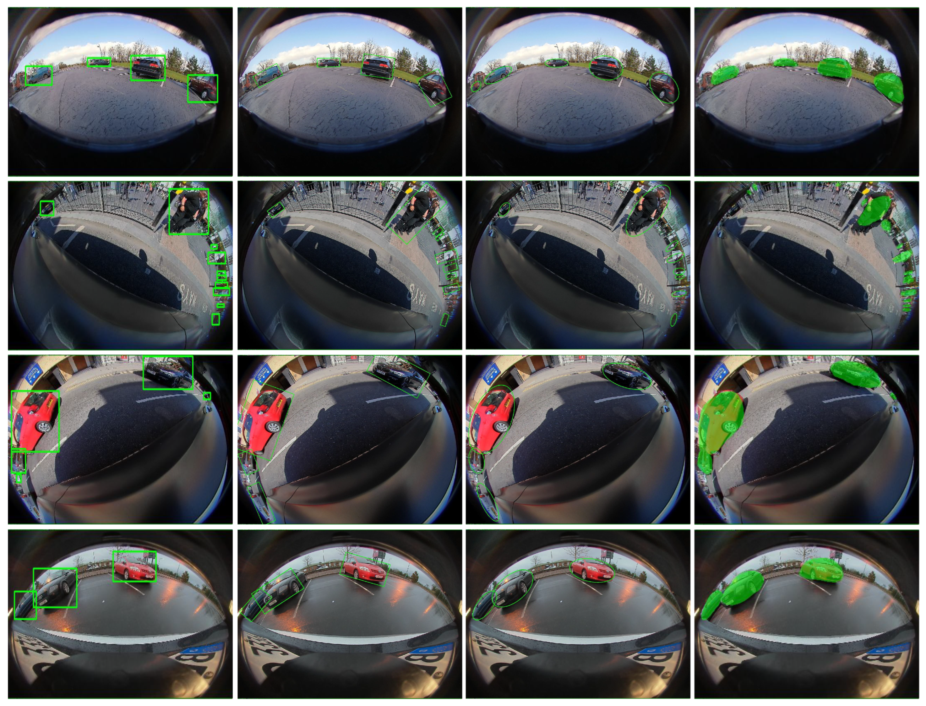
5.3.7. Qualitative Results
5.3.8. Failure Analysis
6. Conclusions
Author Contributions
Funding
Institutional Review Board Statement
Informed Consent Statement
Data Availability Statement
Conflicts of Interest
References
- Joseph, L.; Mondal, A.K. Autonomous Driving and Advanced Driver-Assistance Systems (ADAS): Applications, Development, Legal Issues, and Testing; CRC Press: Boca Raton, FL, USA, 2021. [Google Scholar]
- Kumar, V.R.; Milz, S.; Witt, C.; Simon, M.; Amende, K.; Petzold, J.; Yogamani, S.; Pech, T. Near-field Depth Estimation using Monocular Fisheye Camera: A Semi-supervised learning approach using Sparse LiDAR Data. In Proceedings of the IEEE/CVF Conference on Computer Vision and Pattern Recognition (CVPR) Workshops, Salt Lake City, UT, USA, 18–23 June 2018. [Google Scholar]
- Mohamed, E.; Ewaisha, M.; Siam, M.; Rashed, H.; Yogamani, S.; Hamdy, W.; El-Dakdouky, M.; El-Sallab, A. Monocular instance motion segmentation for autonomous driving: Kitti instancemotseg dataset and multi-task baseline. In Proceedings of the 2021 IEEE Intelligent Vehicles Symposium (IV), Nagoya, Japan, 11–17 July 2021; pp. 114–121. [Google Scholar]
- Yahiaoui, L.; Horgan, J.; Deegan, B.; Yogamani, S.; Hughes, C.; Denny, P. Overview and empirical analysis of ISP parameter tuning for visual perception in autonomous driving. J. Imaging 2019, 5, 78. [Google Scholar] [CrossRef]
- Borse, S.; Klingner, M.; Kumar, V.R.; Cai, H.; Almuzairee, A.; Yogamani, S.; Porikli, F. X-Align: Cross-Modal Cross-View Alignment for Bird’s-Eye-View Segmentation. In Proceedings of the IEEE/CVF Winter Conference on Applications of Computer Vision, Waikoloa, HI, USA, 2–7 January 2023; pp. 3287–3297. [Google Scholar]
- Tripathi, N.; Yogamani, S. Trained trajectory based automated parking system using Visual SLAM. In Proceedings of the Computer Vision and Pattern Recognition Conference Workshops, Nashville, TN, USA, 19–25 June 2021. [Google Scholar]
- LaValle, S.M. Planning Algorithms; Cambridge University Press: Cambridge, UK, 2006. [Google Scholar]
- LaValle, S.M.; Kuffner, J.J., Jr. Randomized kinodynamic planning. Int. J. Robot. Res. 2001, 20, 378–400. [Google Scholar] [CrossRef]
- Schwarting, W.; Alonso-Mora, J.; Rus, D. Planning and decision-making for autonomous vehicles. Annu. Rev. Control. Robot. Auton. Syst. 2018, 1, 187–210. [Google Scholar] [CrossRef]
- Sistu, G.; Leang, I.; Chennupati, S.; Yogamani, S.; Hughes, C.; Milz, S.; Rawashdeh, S. NeurAll: Towards a Unified Visual Perception Model for Automated Driving. In Proceedings of the 2019 IEEE Intelligent Transportation Systems Conference (ITSC), Auckland, New Zealand, 27–30 October 2019; pp. 796–803. [Google Scholar]
- Boulay, T.; El-Hachimi, S.; Surisetti, M.K.; Maddu, P.; Kandan, S. YUVMultiNet: Real-time YUV multi-task CNN for autonomous driving. arXiv 2019, arXiv:1904.05673. [Google Scholar]
- Yogamani, S.; Hughes, C.; Horgan, J.; Sistu, G.; Chennupati, S.; Uricar, M.; Milz, S.; Simon, M.; Amende, K.; Witt, C.; et al. WoodScape: A Multi-Task, Multi-Camera Fisheye Dataset for Autonomous Driving. In Proceedings of the 2019 IEEE/CVF International Conference on Computer Vision (ICCV), Seoul, Republic of Korea, 27 October–2 November 2019. [Google Scholar] [CrossRef]
- Rashed, H.; Mohamed, E.; Sistu, G.; Kumar, V.R.; Eising, C.; El-Sallab, A.; Yogamani, S. Generalized object detection on fisheye cameras for autonomous driving: Dataset, representations and baseline. In Proceedings of the IEEE/CVF Winter Conference on Applications of Computer Vision, Virtual, 5–9 January 2021; pp. 2272–2280. [Google Scholar]
- Girshick, R.; Donahue, J.; Darrell, T.; Malik, J. Rich Feature Hierarchies for Accurate Object Detection and Semantic Segmentation. In Proceedings of the 2014 IEEE Conference on Computer Vision and Pattern Recognition, Columbus, OH, USA, 23–28 June 2014. [Google Scholar] [CrossRef]
- Girshick, R. Fast R-CNN. In Proceedings of the 2015 IEEE International Conference on Computer Vision (ICCV), Santiago, Chile, 7–13 December 2015. [Google Scholar] [CrossRef]
- He, K.; Zhang, X.; Ren, S.; Sun, J. Spatial pyramid pooling in deep convolutional networks for visual recognition. IEEE Trans. Pattern Anal. Mach. Intell. 2015, 37, 1904–1916. [Google Scholar] [CrossRef]
- Ren, S.; He, K.; Girshick, R.; Sun, J. Faster r-cnn: Towards real-time object detection with region proposal networks. In Proceedings of the Advances in Neural Information Processing Systems, Montreal, QC, Canada, 12 December 2015; pp. 91–99. [Google Scholar]
- Dai, J.; Li, Y.; He, K.; Sun, J. R-FCN: Object Detection via Region-based Fully Convolutional Networks. arXiv 2016, arXiv:1605.06409. [Google Scholar]
- Sermanet, P.; Eigen, D.; Zhang, X.; Mathieu, M.; Fergus, R.; LeCun, Y. Overfeat: Integrated recognition, localization and detection using convolutional networks. arXiv 2013, arXiv:1312.6229. [Google Scholar]
- Redmon, J.; Divvala, S.; Girshick, R.; Farhadi, A. You Only Look Once: Unified, Real-Time Object Detection. In Proceedings of the 2016 IEEE Conference on Computer Vision and Pattern Recognition (CVPR), Las Vegas, NV, USA, 27–30 June 2016. [Google Scholar] [CrossRef]
- Redmon, J.; Farhadi, A. YOLO9000: Better, Faster, Stronger. In Proceedings of the 2017 IEEE Conference on Computer Vision and Pattern Recognition (CVPR), Honolulu, HI, USA, 21–26 July 2017. [Google Scholar] [CrossRef]
- Redmon, J.; Farhadi, A. Yolov3: An incremental improvement. arXiv 2018, arXiv:1804.02767. [Google Scholar]
- Liu, W.; Anguelov, D.; Erhan, D.; Szegedy, C.; Reed, S.; Fu, C.Y.; Berg, A.C. Ssd: Single shot multibox detector. In Proceedings of the European Conference on Computer Vision, Milan, Italy, 29 September–4 October 2016; pp. 21–37. [Google Scholar]
- Fu, C.Y.; Liu, W.; Ranga, A.; Tyagi, A.; Berg, A.C. Dssd: Deconvolutional single shot detector. arXiv 2017, arXiv:1701.06659. [Google Scholar]
- Cui, L.; Ma, R.; Lv, P.; Jiang, X.; Gao, Z.; Zhou, B.; Xu, M. Mdssd: Multi-scale deconvolutional single shot detector for small objects. arXiv 2018, arXiv:1805.07009. [Google Scholar] [CrossRef]
- Lin, T.Y.; Goyal, P.; Girshick, R.; He, K.; Dollar, P. Focal Loss for Dense Object Detection. In Proceedings of the 2017 IEEE International Conference on Computer Vision (ICCV), Venice, Italy, 22–29 October 2017. [Google Scholar] [CrossRef]
- He, K.; Gkioxari, G.; Dollar, P.; Girshick, R. Mask R-CNN. In Proceedings of the 2017 IEEE International Conference on Computer Vision (ICCV), Venice, Italy, 22–29 October 2017. [Google Scholar] [CrossRef]
- Dai, J.; He, K.; Sun, J. Instance-Aware Semantic Segmentation via Multi-task Network Cascades. In Proceedings of the 2016 IEEE Conference on Computer Vision and Pattern Recognition (CVPR), Las Vegas, NV, USA, 27–30 June 2016. [Google Scholar] [CrossRef]
- Xie, E.; Sun, P.; Song, X.; Wang, W.; Liu, X.; Liang, D.; Shen, C.; Luo, P. Polarmask: Single shot instance segmentation with polar representation. In Proceedings of the IEEE/CVF Conference on Computer Vision and Pattern Recognition, Seattle, WA, USA, 13–19 June 2020; pp. 12193–12202. [Google Scholar]
- Bolya, D.; Zhou, C.; Xiao, F.; Lee, Y.J. Yolact: Real-time instance segmentation. In Proceedings of the IEEE International Conference on Computer Vision, Seoul, Republic of Korea, 27 October–2 November 2019; pp. 9157–9166. [Google Scholar]
- Hurtik, P.; Molek, V.; Hula, J.; Vajgl, M.; Vlasanek, P.; Nejezchleba, T. Poly-YOLO: Higher speed, more precise detection and instance segmentation for YOLOv3. arXiv 2020, arXiv:2005.13243. [Google Scholar] [CrossRef]
- He, K.; Zhang, X.; Ren, S.; Sun, J. Deep residual learning for image recognition. In Proceedings of the IEEE Conference on Computer Vision and Pattern Recognition, Las Vegas, NV, USA, 27–30 June 2016; pp. 770–778. [Google Scholar]
- Liang, X.; Lin, L.; Wei, Y.; Shen, X.; Yang, J.; Yan, S. Proposal-Free Network for Instance-Level Object Segmentation. IEEE Trans. Pattern Anal. Mach. Intell. 2018, 40, 2978–2991. [Google Scholar] [CrossRef] [PubMed]
- Neven, D.; Brabandere, B.D.; Proesmans, M.; Van Gool, L. Instance Segmentation by Jointly Optimizing Spatial Embeddings and Clustering Bandwidth. In Proceedings of the 2019 IEEE/CVF Conference on Computer Vision and Pattern Recognition (CVPR), Long Beach, CA, USA, 15–20 June 2019. [Google Scholar] [CrossRef]
- Cheng, B.; Collins, M.D.; Zhu, Y.; Liu, T.; Huang, T.S.; Adam, H.; Chen, L.C. Panoptic-DeepLab: A Simple, Strong, and Fast Baseline for Bottom-Up Panoptic Segmentation. In Proceedings of the 2020 IEEE/CVF Conference on Computer Vision and Pattern Recognition (CVPR), Seattle, WA, USA, 13–19 June 2020. [Google Scholar] [CrossRef]
- Ankerst, M.; Breunig, M.M.; Kriegel, H.P.; Sander, J. OPTICS: Ordering Points to Identify the Clustering Structure. In Proceedings of the 1999 ACM SIGMOD International Conference on Management of Data, Philadelphia, PA, USA, 1–3 June 1999; SIGMOD ’99. pp. 49–60. [Google Scholar] [CrossRef]
- Ester, M.; Kriegel, H.P.; Sander, J.; Xu, X. A density-based algorithm for discovering clusters in large spatial databases with noise. In Proceedings of the Kdd, Portland, OR, USA, 2–4 August 1996; Volume 96, pp. 226–231. [Google Scholar]
- Ramachandran, S.; Sistu, G.; Kumar, V.R.; McDonald, J.; Yogamani, S. Woodscape Fisheye Object Detection for Autonomous Driving–CVPR 2022 OmniCV Workshop Challenge. arXiv 2022, arXiv:2206.12912. [Google Scholar]
- Li, T.; Tong, G.; Tang, H.; Li, B.; Chen, B. FisheyeDet: A Self-Study and Contour-Based Object Detector in Fisheye Images. IEEE Access 2020, 8, 71739–71751. [Google Scholar] [CrossRef]
- Everingham, M.; Van Gool, L.; Williams, C.K.; Winn, J.; Zisserman, A. The pascal visual object classes (voc) challenge. Int. J. Comput. Vis. 2010, 88, 303–338. [Google Scholar] [CrossRef]
- Coors, B.; Paul Condurache, A.; Geiger, A. SphereNet: Learning spherical representations for detection and classification in omnidirectional images. In Proceedings of the European Conference on Computer Vision (ECCV), Munich, Germany, 8–14 September 2018. [Google Scholar]
- Perraudin, N.; Defferrard, M.; Kacprzak, T.; Sgier, R. DeepSphere: Efficient spherical convolutional neural network with HEALPix sampling for cosmological applications. Astron. Comput. 2019, 27, 130–146. [Google Scholar] [CrossRef]
- Su, Y.C.; Grauman, K. Kernel transformer networks for compact spherical convolution. In Proceedings of the IEEE Conference on Computer Vision and Pattern Recognition, Long Beach, CA, USA, 15–20 June 2019. [Google Scholar]
- Jiang, C.; Huang, J.; Kashinath, K.; Prabhat; Marcus, P.; Niessner, M. Spherical CNNs on unstructured grids. arXiv 2019, arXiv:1901.02039. [Google Scholar]
- Kumar, V.R.; Klingner, M.; Yogamani, S.; Bach, M.; Milz, S.; Fingscheidt, T.; Mäder, P. SVDistNet: Self-supervised near-field distance estimation on surround view fisheye cameras. IEEE Trans. Intell. Transp. Syst. 2021, 23, 10252–10261. [Google Scholar] [CrossRef]
- Rashed, H.; Mohamed, E.; Sistu, G.; Kumar, V.R.; Eising, C.; El-Sallab, A.; Yogamani, S. FisheyeYOLO: Object detection on fisheye cameras for autonomous driving. In Proceedings of the Machine Learning for Autonomous Driving NeurIPS 2020 Virtual Workshop, Virtual, 11 December 2020; Volume 11. [Google Scholar]
- Zhao, H.; Jia, J.; Koltun, V. Exploring self-attention for image recognition. In Proceedings of the 2020 IEEE/CVF Conference on Computer Vision and Pattern Recognition (CVPR), Seattle, WA, USA, 13–19 June 2020. [Google Scholar]
- Kumar, V.R.; Yogamani, S.; Bach, M.; Witt, C.; Milz, S.; Mader, P. UnRectDepthNet: Self-Supervised Monocular Depth Estimation using a Generic Framework for Handling Common Camera Distortion Models. In Proceedings of the 2020 IEEE/RSJ International Conference on Intelligent Robots and Systems (IROS 2020), Las Vegas, NV, USA, 25–29 October 2020. [Google Scholar]
- Liu, R.; Lehman, J.; Molino, P.; Such, F.P.; Frank, E.; Sergeev, A.; Yosinski, J. An Intriguing Failing of Convolutional Neural Networks and the Coordconv solution. In Proceedings of the 32nd International Conference on Neural Information Processing Systems, Montréal, QC, Canada, 3–8 December 2018. [Google Scholar]
- Facil, J.M.; Ummenhofer, B.; Zhou, H.; Montesano, L.; Brox, T.; Civera, J. CAM-Convs: Camera-Aware Multi-Scale Convolutions for Single-View Depth. In Proceedings of the 2019 IEEE/CVF Conference on Computer Vision and Pattern Recognition (CVPR), Long Beach, CA, USA, 15–20 June 2019. [Google Scholar]
- Teh, C.H.; Chin, R.T. On the detection of dominant points on digital curves. IEEE Trans. Pattern Anal. Mach. Intell. 1989, 11, 859–872. [Google Scholar] [CrossRef]
- Douglas, D.H.; Peucker, T.K. Algorithms for the reduction of the number of points required to represent a digitized line or its caricature. In Proceedings of the Cartographica: The International Journal for Geographic Information and Geovisualization; University of Toronto Press: Toronto, ON, Canada, 1973. [Google Scholar]
- Hughes, C.; McFeely, R.; Denny, P.; Glavin, M.; Jones, E. Equidistant fish-eye perspective with application in distortion centre estimation. In Proceedings of the 18th International Vacuum Congress (IVC-18), Beijing, China, 23–27 August 2010. [Google Scholar]
- Bräuer-Burchardt, C.; Voss, K. A new algorithm to correct fish-eye- and strong wide-angle-lens-distortion from single images. In Proceedings of the 2001 International Conference on Image Processing, Thessaloniki, Greece, 7–10 October 2001. [Google Scholar]
- Scaramuzza, D.; Martinelli, A.; Siegwart, R. A flexible technique for accurate omnidirectional camera calibration and structure from motion. In Proceedings of the IEEE International Conference on Computer Vision Systems, New York, NY, USA, 4–7 January 2006. [Google Scholar]
- Manzoor, A.; Mohandas, R.; Scanlan, A.; Grua, E.M.; Collins, F.; Sistu, G.; Eising, C. A Comparison of Spherical Neural Networks for Surround-view Fisheye Image Semantic Segmentation. IEEE Open J. Veh. Technol. 2025, 6, 717–740. [Google Scholar] [CrossRef]
- Uricár, M.; Hurych, D.; Krizek, P.; Yogamani, S. Challenges in designing datasets and validation for autonomous driving. In Proceedings of the International Joint Conference on Computer Vision, Imaging and Computer Graphics Theory and Applications (VISAPP), Prague, Czech Republic, 25–27 February 2019. [Google Scholar]
- Paszke, A.; Gross, S.; Massa, F.; Lerer, A.; Bradbury, J.; Chanan, G.; Killeen, T.; Lin, Z.; Gimelshein, N.; Antiga, L.; et al. Pytorch: An imperative style, high-performance deep learning library. In Proceedings of the Advances in Neural Information Processing Systems, Vancouver, BC, Canada, 8–14 December 2019; pp. 8026–8037. [Google Scholar]
- Yong, H.; Huang, J.; Hua, X.; Zhang, L. Gradient Centralization: A New Optimization Technique for Deep Neural Networks. arXiv 2020, arXiv:2004.01461. [Google Scholar]
- Smith, L.N. A disciplined approach to neural network hyper-parameters: Part 1—Learning rate, batch size, momentum, and weight decay. arXiv 2018, arXiv:1803.09820. [Google Scholar]
- Liu, L.; Jiang, H.; He, P.; Chen, W.; Liu, X.; Gao, J.; Han, J. On the variance of the adaptive learning rate and beyond. arXiv 2019, arXiv:1908.03265. [Google Scholar]
- Zhang, M.R.; Lucas, J.; Hinton, G.; Ba, J. Lookahead Optimizer: k steps forward, 1 step back. arXiv 2019, arXiv:1907.08610. [Google Scholar]

| Representation | mIoU | mIoU | No. of Params | |||
|---|---|---|---|---|---|---|
| Front | Rear | Left | Right | |||
| Bounding Box | 53.7 | 47.9 | 60.6 | 43.2 | 51.4 | 4 |
| Oriented Box | 55.0 | 50.2 | 64.8 | 45.9 | 53.9 | 5 |
| Ellipse | 56.5 | 51.7 | 66.5 | 47.5 | 55.5 | 5 |
| 24-sided Polygon (uniform) | 85.0 | 84.9 | 83.9 | 83.8 | 84.4 | 48 |
| 24-sided Polygon (adaptive) | 87.2 | 87 | 86.2 | 86.1 | 86.6 | 48 |
| Experiment | Representation vs. Representation | Representation vs. Segmentation Mask | ||||
|---|---|---|---|---|---|---|
| Vehicle | Pedestrian | mAP | Vehicle | Pedestrian | mAP | |
| Bounding Box | 66.3 | 31.6 | 48.9 | 51.3 | 31.5 | 41.4 |
| Oriented Box | 65.5 | 30.1 | 47.8 | 52.3 | 31.9 | 42.1 |
| Ellipse | 66 | 29 | 47.5 | 52.9 | 28.9 | 40.9 |
| Polygon (24 points) | 66.2 | 31.4 | 48.8 | 67.6 | 31.6 | 49.6 |
| Representation | Annotation Time (s) | Inference Time (fps) | Training Time (h) |
|---|---|---|---|
| Bounding Box | 2.1 | 49 | 8 |
| Oriented Box/Ellipse | 3.1 | 52 | 8 |
| Curved Box | 3.5 | 52 | 9.5 |
| 24-sided Polygon | 41.6 | 56 | 26 |
| Configuration | mAP |
|---|---|
| Oriented Box | |
| Orientation regression | 39 |
| Orientation classification | 40.6 |
| Orientation classification + IoU loss | 41.9 |
| 24-sided Polygon | |
| Uniform Angular | 55.6 |
| Uniform Perimeter | 55.4 |
| Adaptive Perimeter | 58.1 |
| Encoder Type | |
| ResNet18 | 58.1 |
| SAN-10 | 58.8 |
| SAN-19 | 59.3 |
| Number of streams | |
| Single | 58.1 |
| Two stream | 58.7 |
| Camera Geometry Tensor | |
| Without CGT | 58.1 |
| With CGT | 59.5 |
| Effect of Undistortion for Bounding Box | |
| Rectilinear | 39.8 |
| Cylindrical | 43.7 |
| No undistortion | 45.4 |
| Effect of Undistortion for 24-polygon | |
| Rectilinear | 52.2 |
| Cylindrical | 57.2 |
| No undistortion | 58.1 |
| Representation | IoU | mIoU | |||
|---|---|---|---|---|---|
| Front | Rear | Left | Right | ||
| Bounding Box | 32.5 | 32.1 | 34.2 | 27.8 | 31.6 |
| Oriented Box | 33.9 | 33.5 | 37.2 | 30.1 | 33.2 |
| Curved Box | 33 | 32.7 | 35.4 | 28 | 32.3 |
| Vanishing point guided Curved Box | 34.3 | 34.1 | 38.3 | 32.4 | 34.8 |
Disclaimer/Publisher’s Note: The statements, opinions and data contained in all publications are solely those of the individual author(s) and contributor(s) and not of MDPI and/or the editor(s). MDPI and/or the editor(s) disclaim responsibility for any injury to people or property resulting from any ideas, methods, instructions or products referred to in the content. |
© 2025 by the authors. Licensee MDPI, Basel, Switzerland. This article is an open access article distributed under the terms and conditions of the Creative Commons Attribution (CC BY) license (https://creativecommons.org/licenses/by/4.0/).
Share and Cite
Yogamani, S.; Sistu, G.; Denny, P.; Courtney, J. Let’s Go Bananas: Beyond Bounding Box Representations for Fisheye Camera-Based Object Detection in Autonomous Driving. Sensors 2025, 25, 3735. https://doi.org/10.3390/s25123735
Yogamani S, Sistu G, Denny P, Courtney J. Let’s Go Bananas: Beyond Bounding Box Representations for Fisheye Camera-Based Object Detection in Autonomous Driving. Sensors. 2025; 25(12):3735. https://doi.org/10.3390/s25123735
Chicago/Turabian StyleYogamani, Senthil, Ganesh Sistu, Patrick Denny, and Jane Courtney. 2025. "Let’s Go Bananas: Beyond Bounding Box Representations for Fisheye Camera-Based Object Detection in Autonomous Driving" Sensors 25, no. 12: 3735. https://doi.org/10.3390/s25123735
APA StyleYogamani, S., Sistu, G., Denny, P., & Courtney, J. (2025). Let’s Go Bananas: Beyond Bounding Box Representations for Fisheye Camera-Based Object Detection in Autonomous Driving. Sensors, 25(12), 3735. https://doi.org/10.3390/s25123735