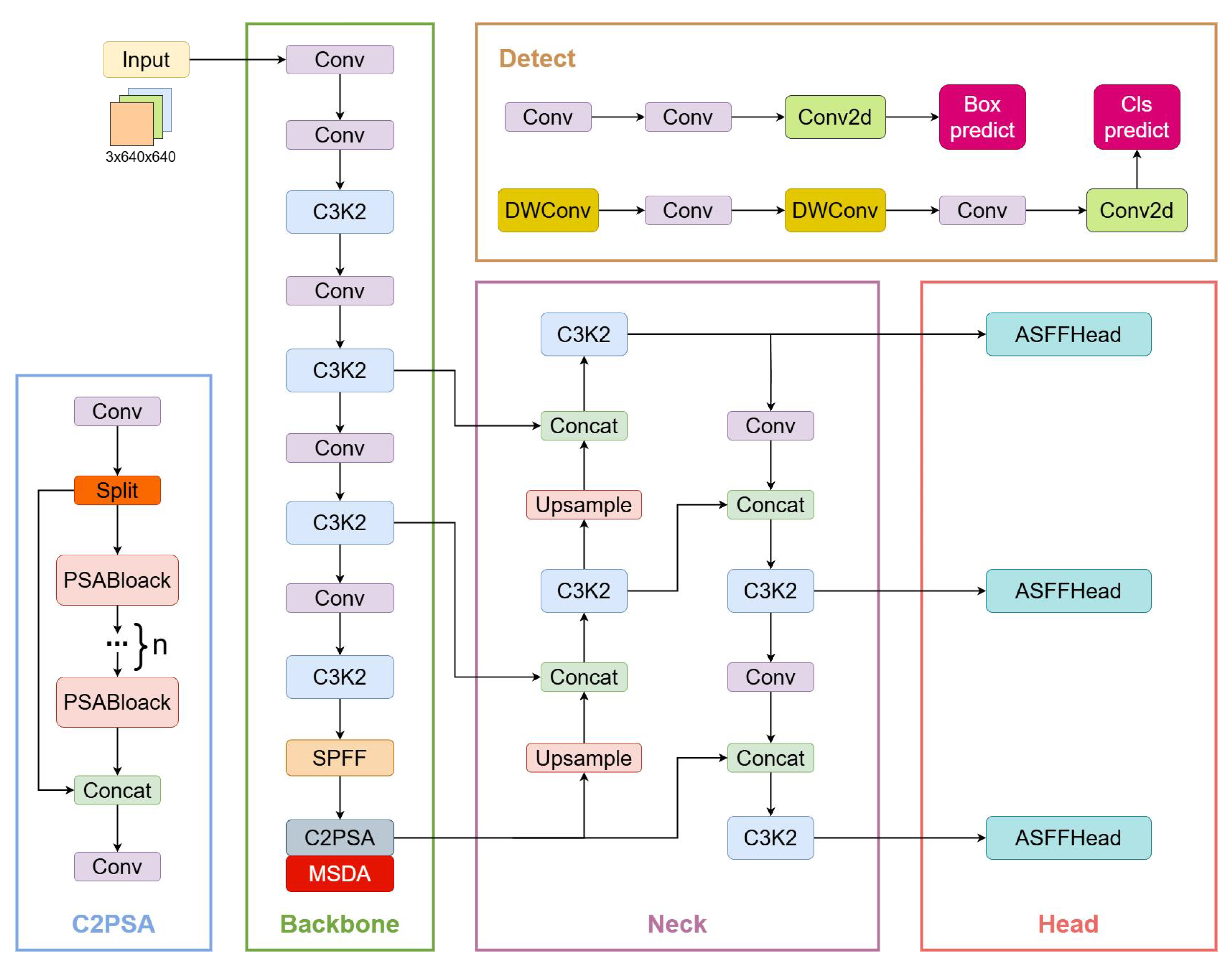
Figure 1.
MAS-YOLOv11 model, where the MSDA was embedded in the C2PSA module and the original YOLO v11 detection head was replaced with ASFFHead.
Figure 1.
MAS-YOLOv11 model, where the MSDA was embedded in the C2PSA module and the original YOLO v11 detection head was replaced with ASFFHead.
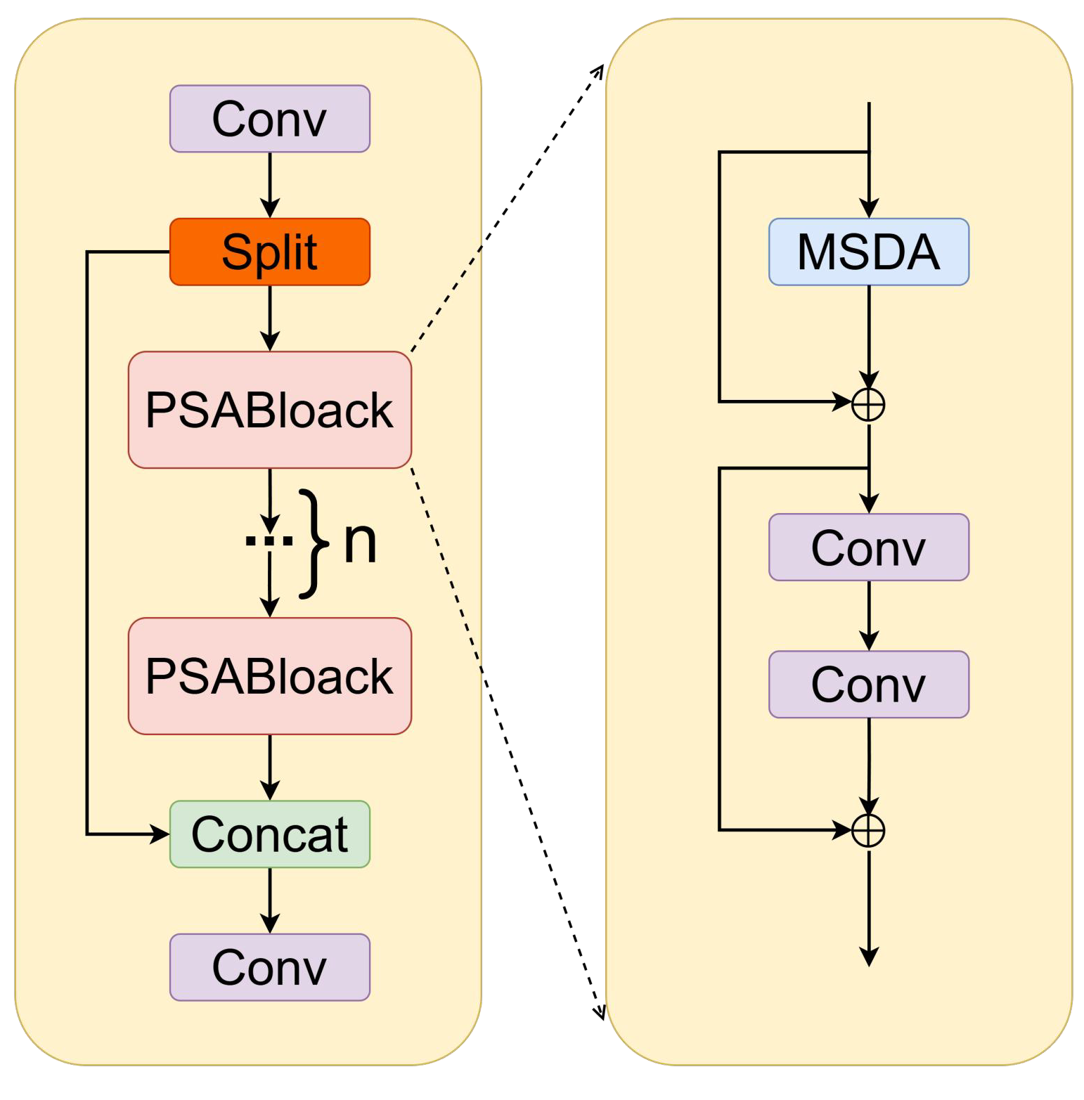
Figure 2.
C2PSA_MSDA module.
Figure 2.
C2PSA_MSDA module.
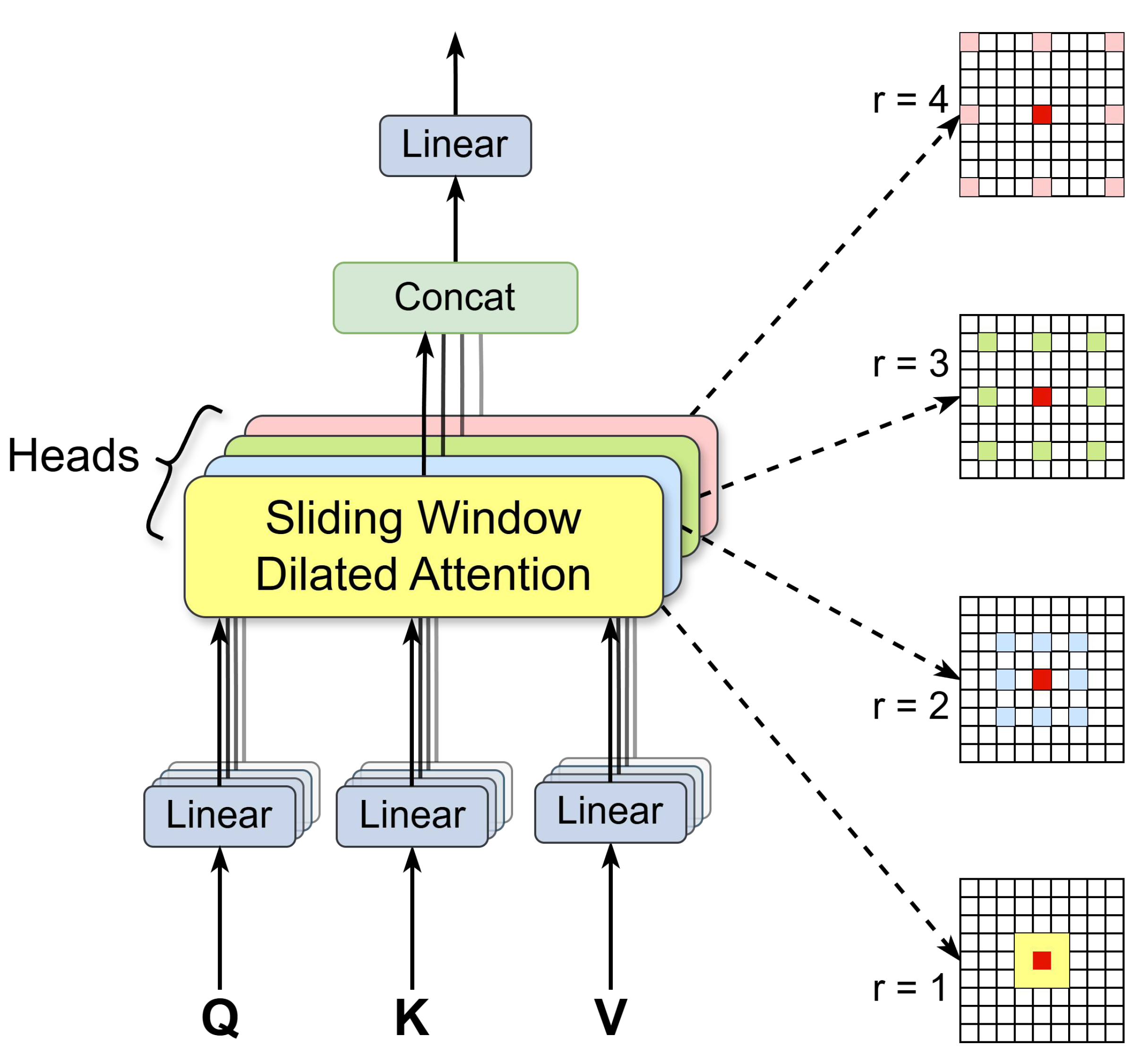
Figure 3.
MSDA module, which describes the working principle of MSDA in the C2PSA_MSDA module. First, the feature map channels are split into multiple heads. Each head performs a self-attention operation on a query patch within a colored region centered on a red window, using a distinct dilation rate. The features from different heads are then concatenated and passed through a linear layer. By default, we use four dilation rates: r = 1, 2, 3, and 4, corresponding to receptive field sizes of 3 × 3, 5 × 5, 7 × 7, and 9 × 9, respectively.
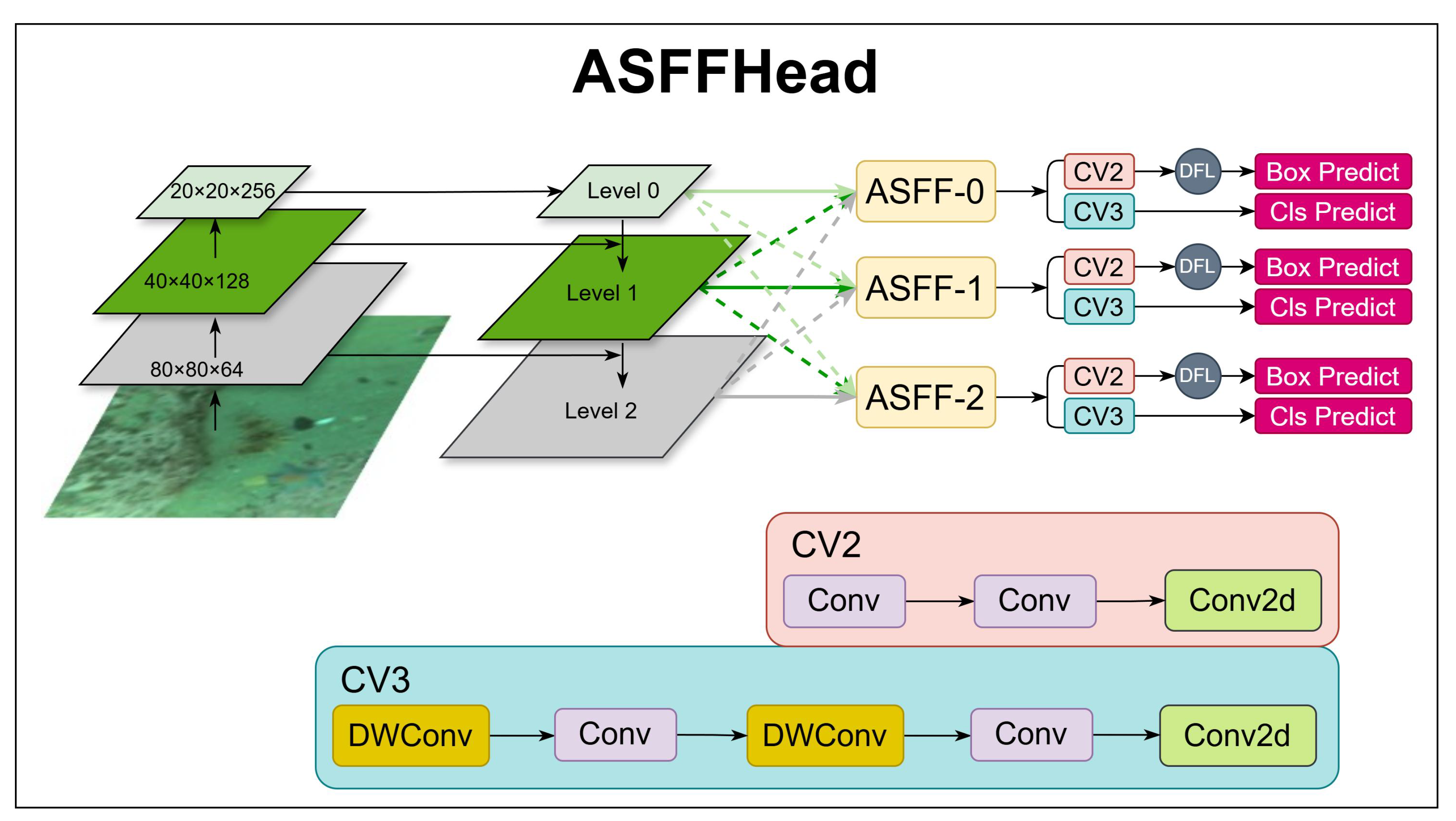
Figure 4.
ASFFHead structure describing the ASFFHead workflow.
Figure 4.
ASFFHead structure describing the ASFFHead workflow.
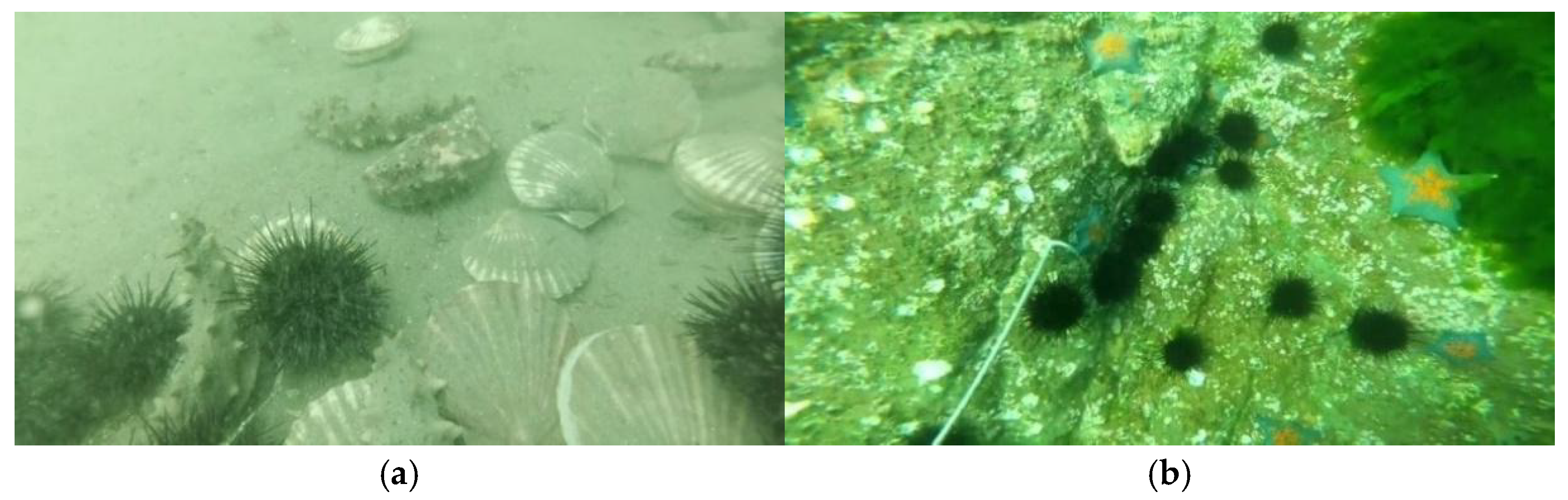
Figure 5.
This is a sample image of the DUO dataset, in which (a) the image has degraded problems such as blurring and color cast, including holothurian, echinus, and scallop categories, and (b) the image has severe color cast, including starfish and echinus.
Figure 5.
This is a sample image of the DUO dataset, in which (a) the image has degraded problems such as blurring and color cast, including holothurian, echinus, and scallop categories, and (b) the image has severe color cast, including starfish and echinus.
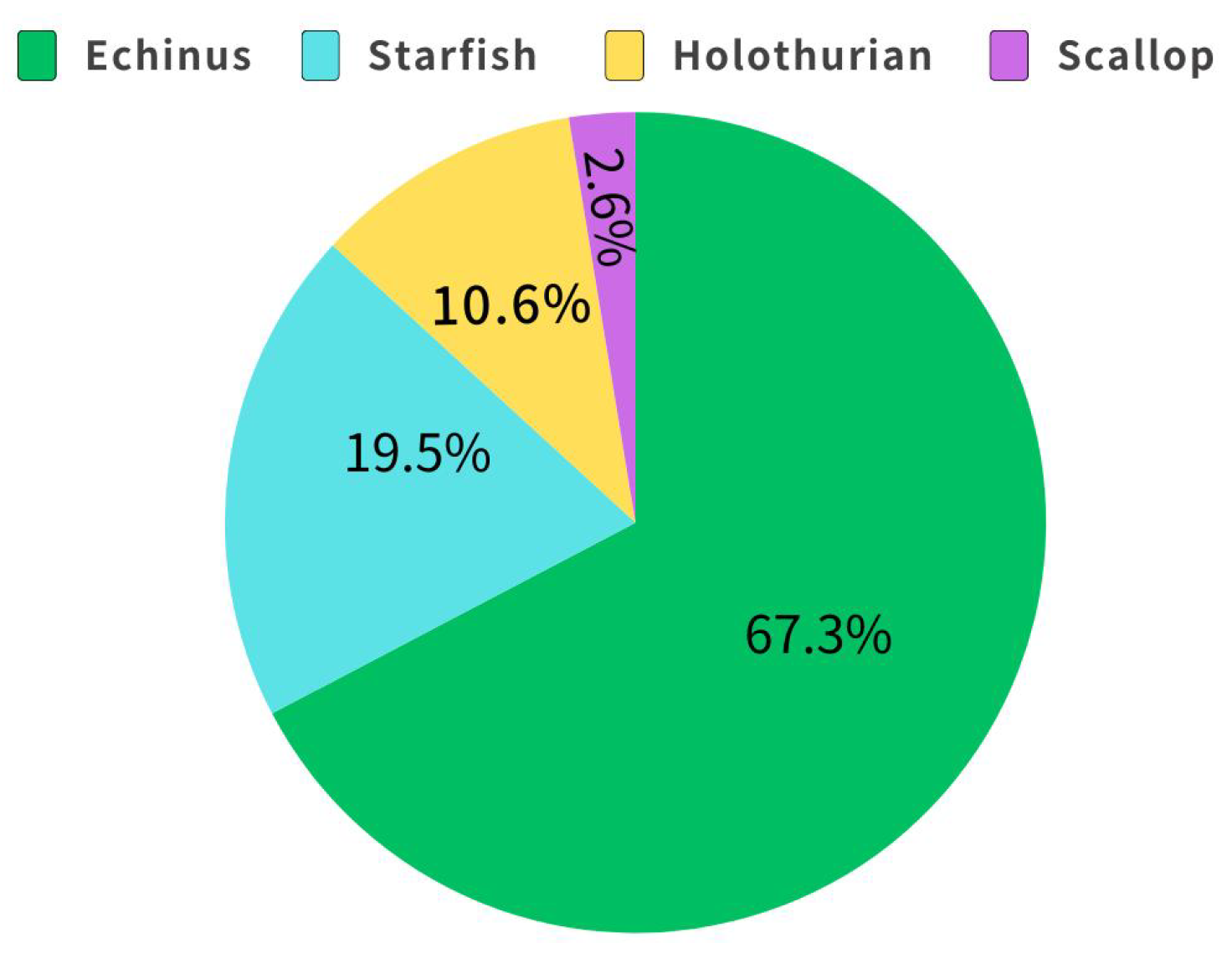
Figure 6.
The distribution of the number of labeled objects by category in DUO.
Figure 6.
The distribution of the number of labeled objects by category in DUO.
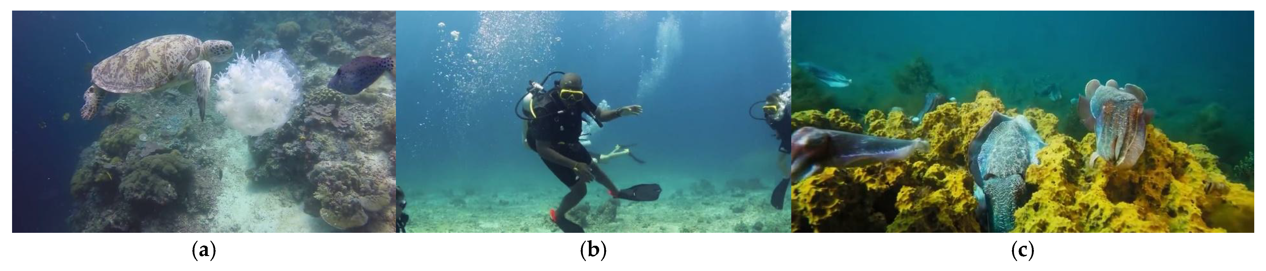
Figure 7.
This is a sample of the RUOD dataset, where (a–c) are the categories of the redundant DUO dataset: (a) fish, turtles, and jellyfish; (b) divers; (c) corals and squid.
Figure 7.
This is a sample of the RUOD dataset, where (a–c) are the categories of the redundant DUO dataset: (a) fish, turtles, and jellyfish; (b) divers; (c) corals and squid.
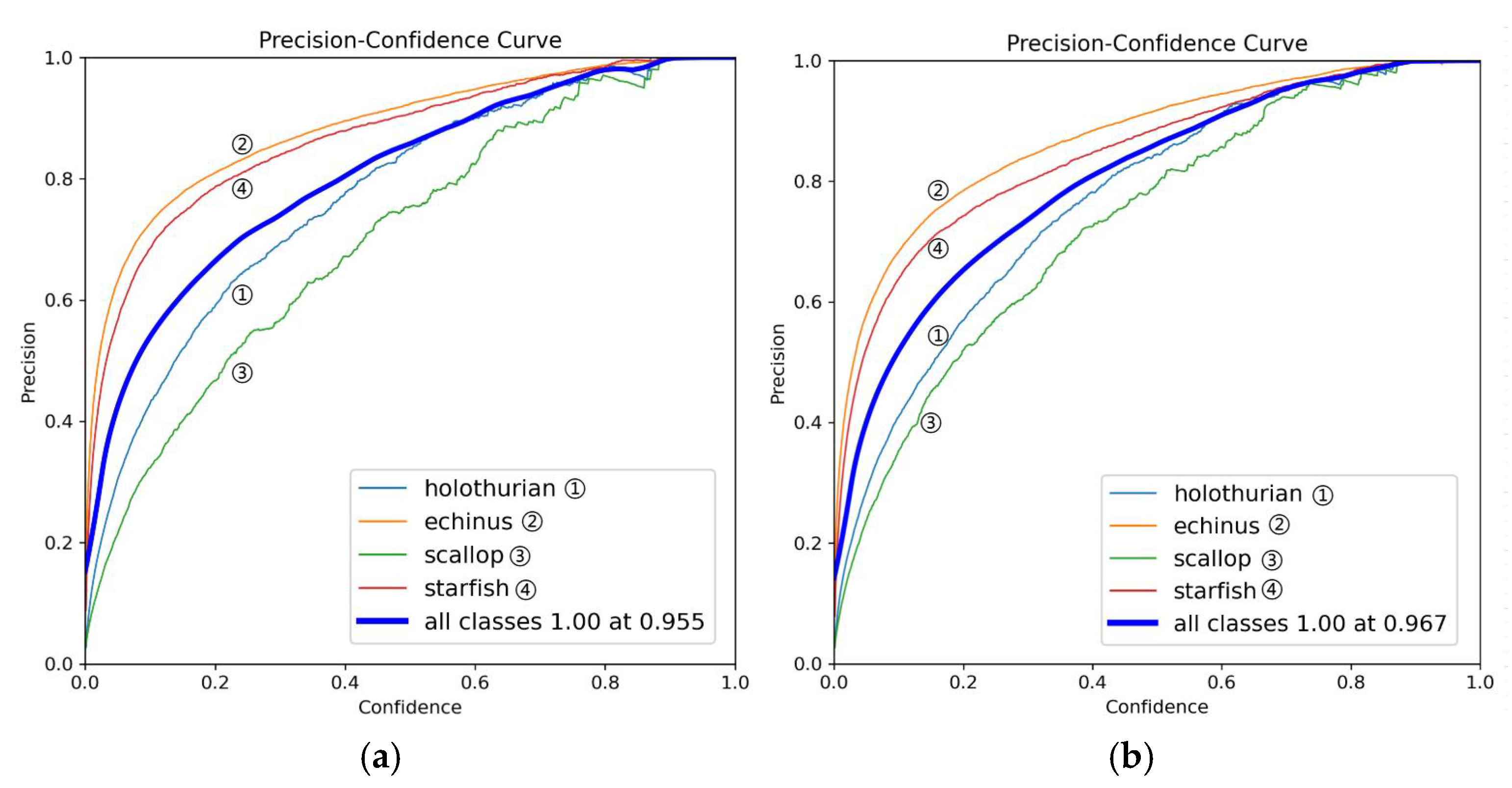
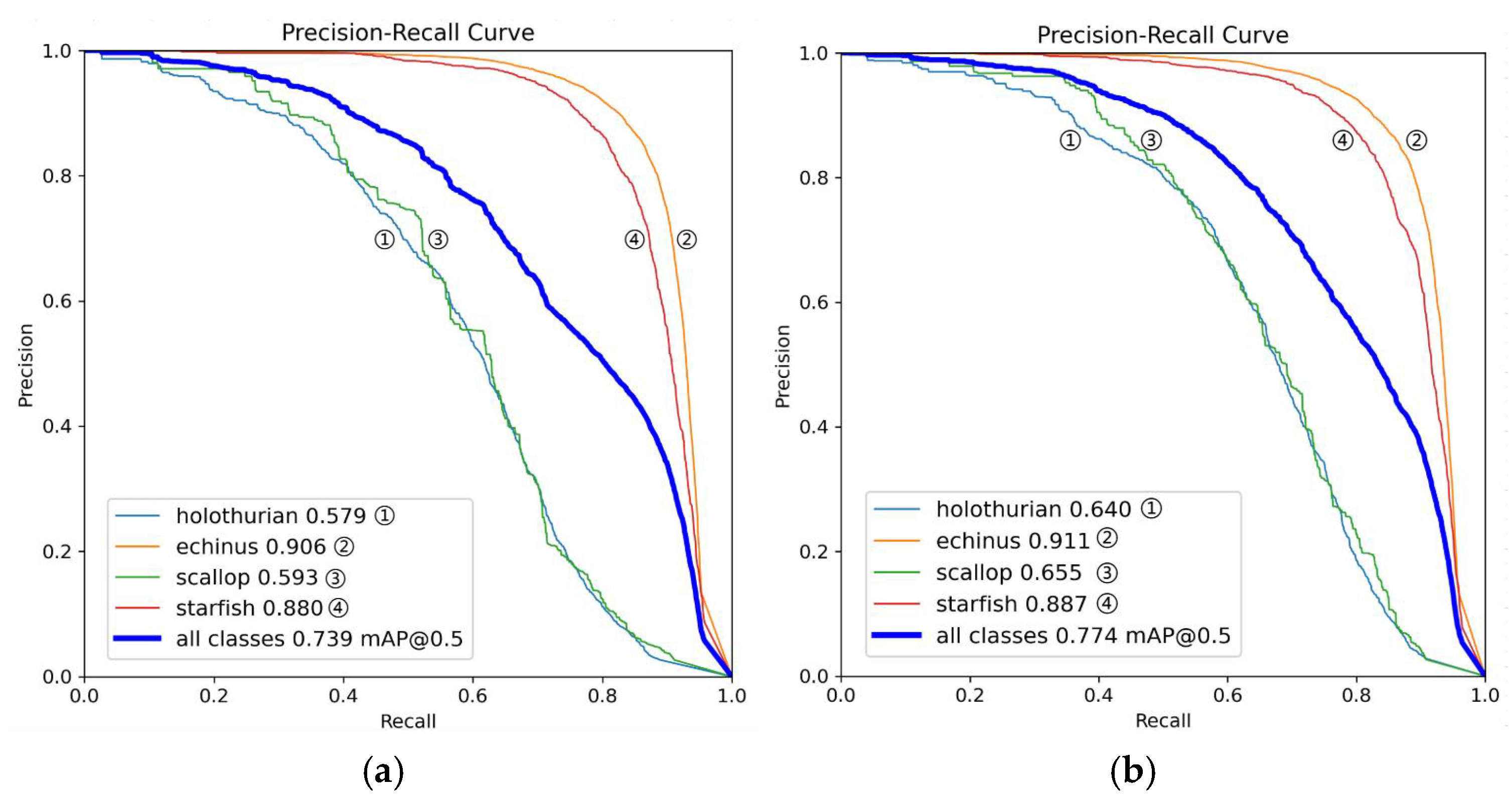
Figure 8.
This is a precision comparison chart, where (a) is the YOLOv11 model and (b) is the MAS-YOLOv11 model.
Figure 8.
This is a precision comparison chart, where (a) is the YOLOv11 model and (b) is the MAS-YOLOv11 model.
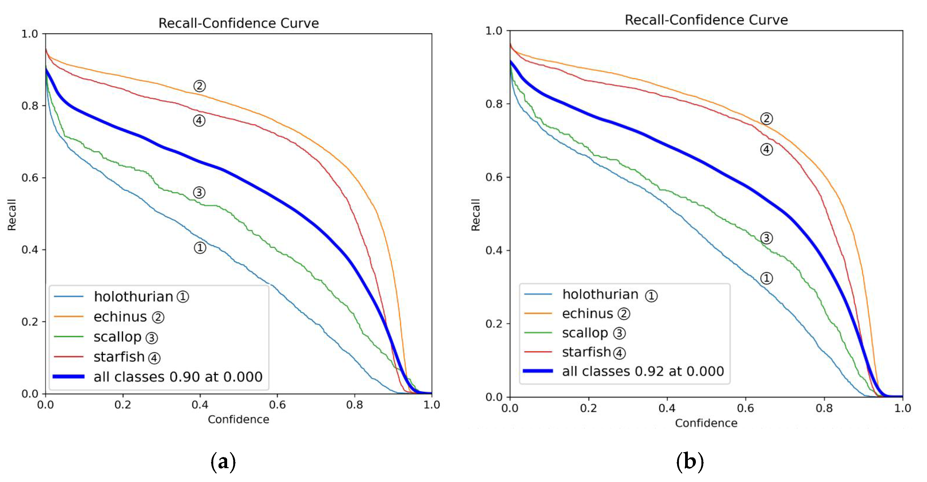
Figure 9.
This is a recall comparison chart, where (a) is the YOLOv11 model and (b) is the MAS-YOLOv11 model.
Figure 9.
This is a recall comparison chart, where (a) is the YOLOv11 model and (b) is the MAS-YOLOv11 model.
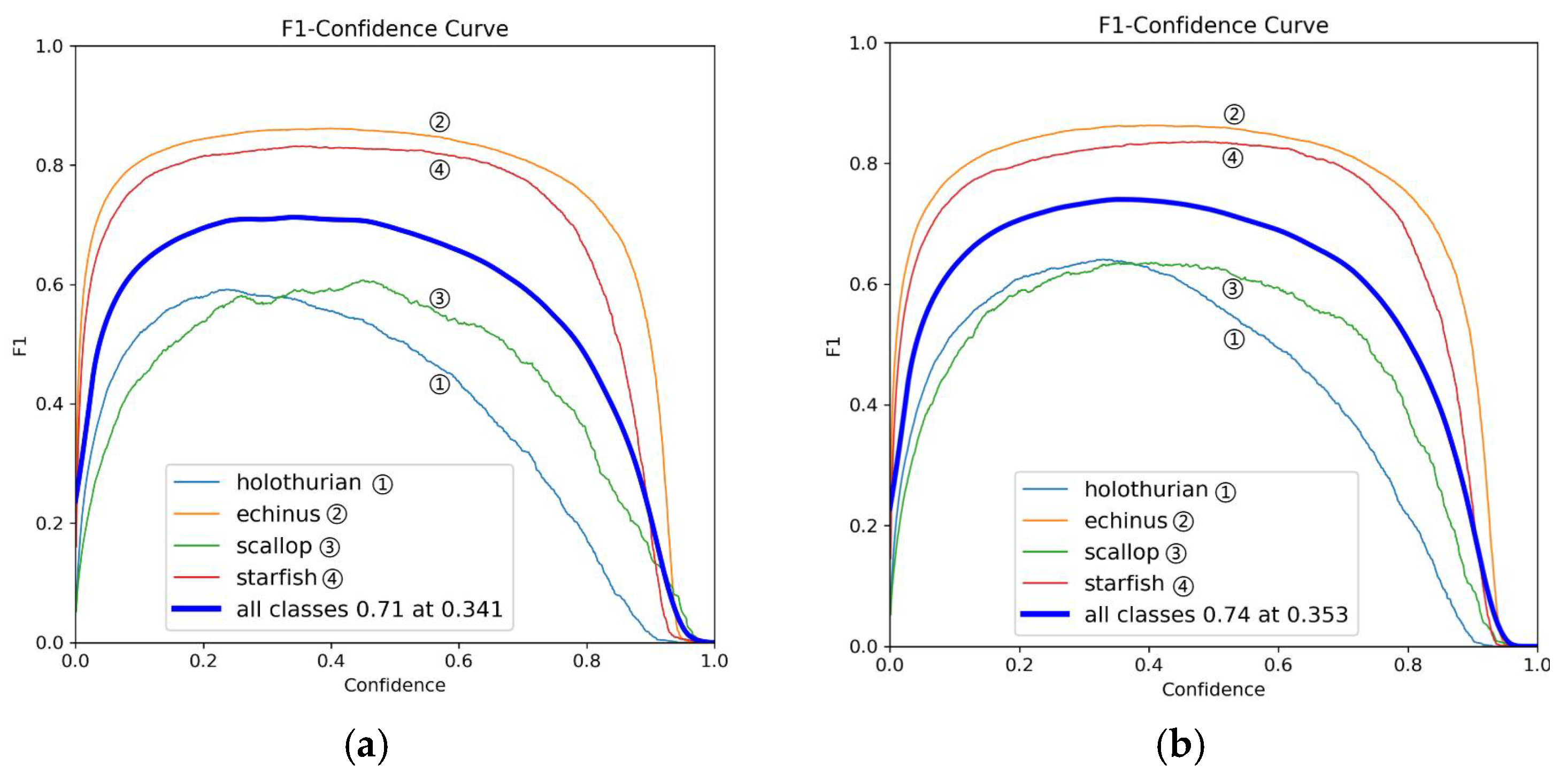
Figure 10.
This is an F1 comparison chart, where (a) is the YOLOv11 model and (b) is the MAS-YOLOv11 model.
Figure 10.
This is an F1 comparison chart, where (a) is the YOLOv11 model and (b) is the MAS-YOLOv11 model.
Figure 11.
This is an mAP@50 comparison chart, where (a) is the YOLOv11 model and (b) is the MAS-YOLOv11 model.
Figure 11.
This is an mAP@50 comparison chart, where (a) is the YOLOv11 model and (b) is the MAS-YOLOv11 model.
Figure 12.
This is a RUOD result chart, where (a) is a precision plot, (b) is a recall plot, (c) is an F1 plot, (d) is an mAP@50 plot, and (e) is an example of a test results plot.
Figure 12.
This is a RUOD result chart, where (a) is a precision plot, (b) is a recall plot, (c) is an F1 plot, (d) is an mAP@50 plot, and (e) is an example of a test results plot.
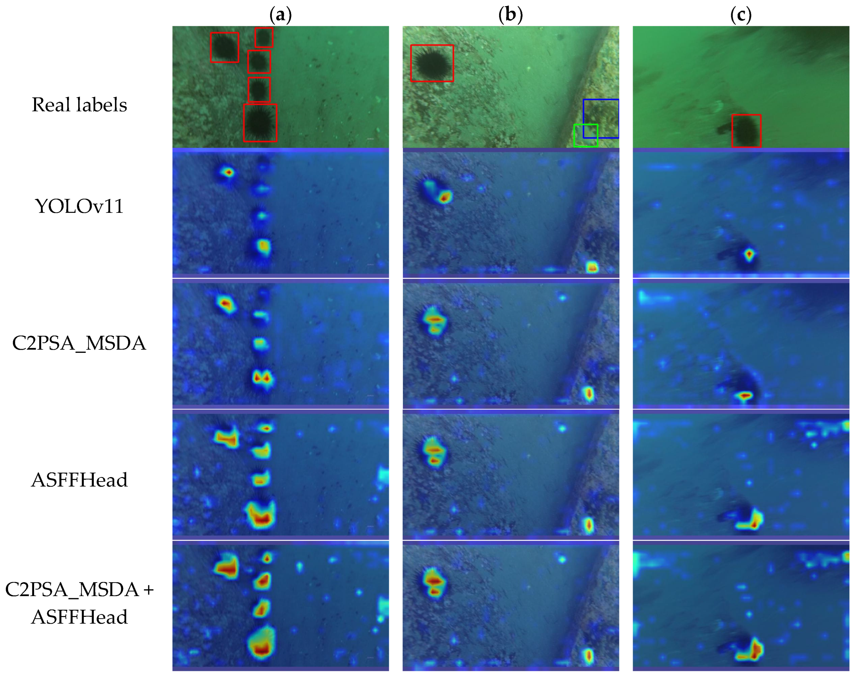
Figure 13.
This is the Grad-CAM heatmap of MAS-YOLOv11, where (a) is a dense target with occlusion, (b) is a sparsely distributed multi-category target, and (c) is a blurred target.
Figure 13.
This is the Grad-CAM heatmap of MAS-YOLOv11, where (a) is a dense target with occlusion, (b) is a sparsely distributed multi-category target, and (c) is a blurred target.
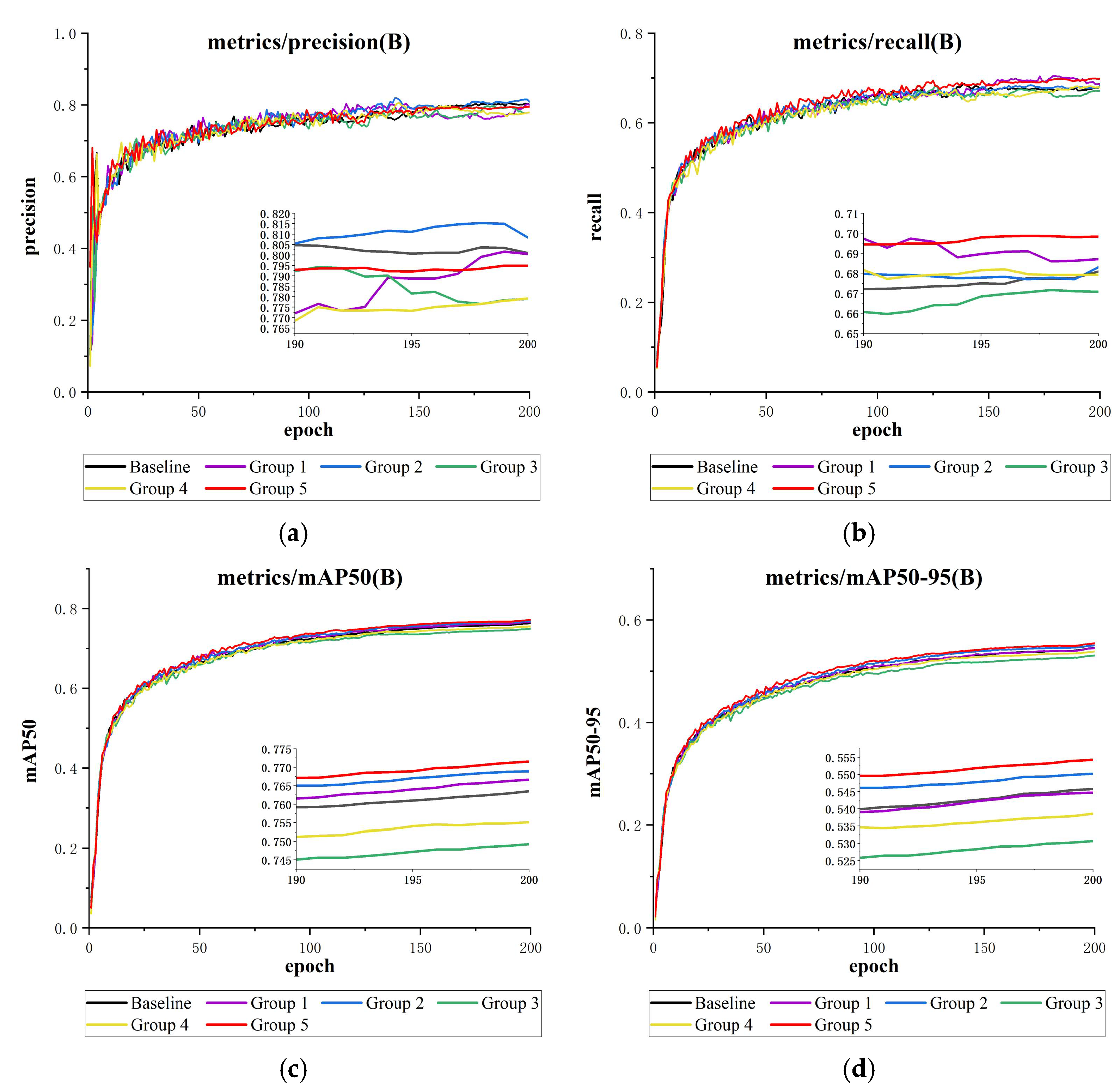
Figure 14.
This is a comparison of the attention mechanisms’ results charts (containing detailed subgraphs for 190–200 epochs): (a) precision comparison, (b) recall comparison, (c) mAP@50 comparison, and (d) mAP@50-95 comparison.
Figure 14.
This is a comparison of the attention mechanisms’ results charts (containing detailed subgraphs for 190–200 epochs): (a) precision comparison, (b) recall comparison, (c) mAP@50 comparison, and (d) mAP@50-95 comparison.
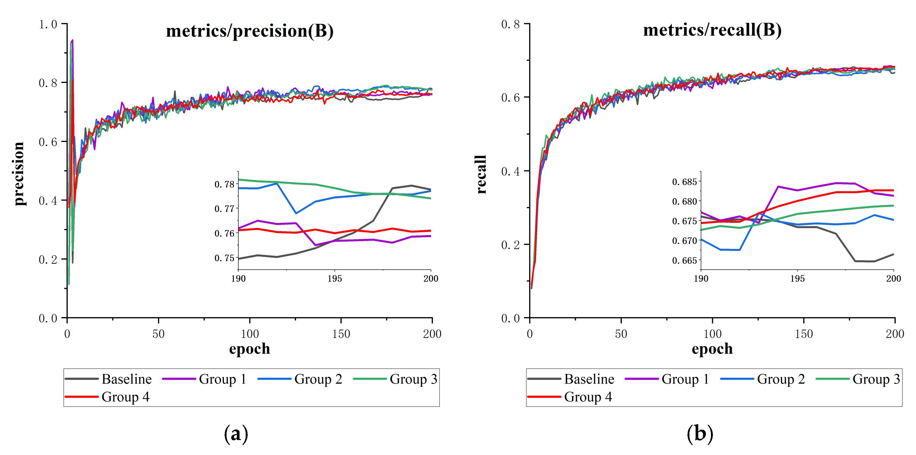
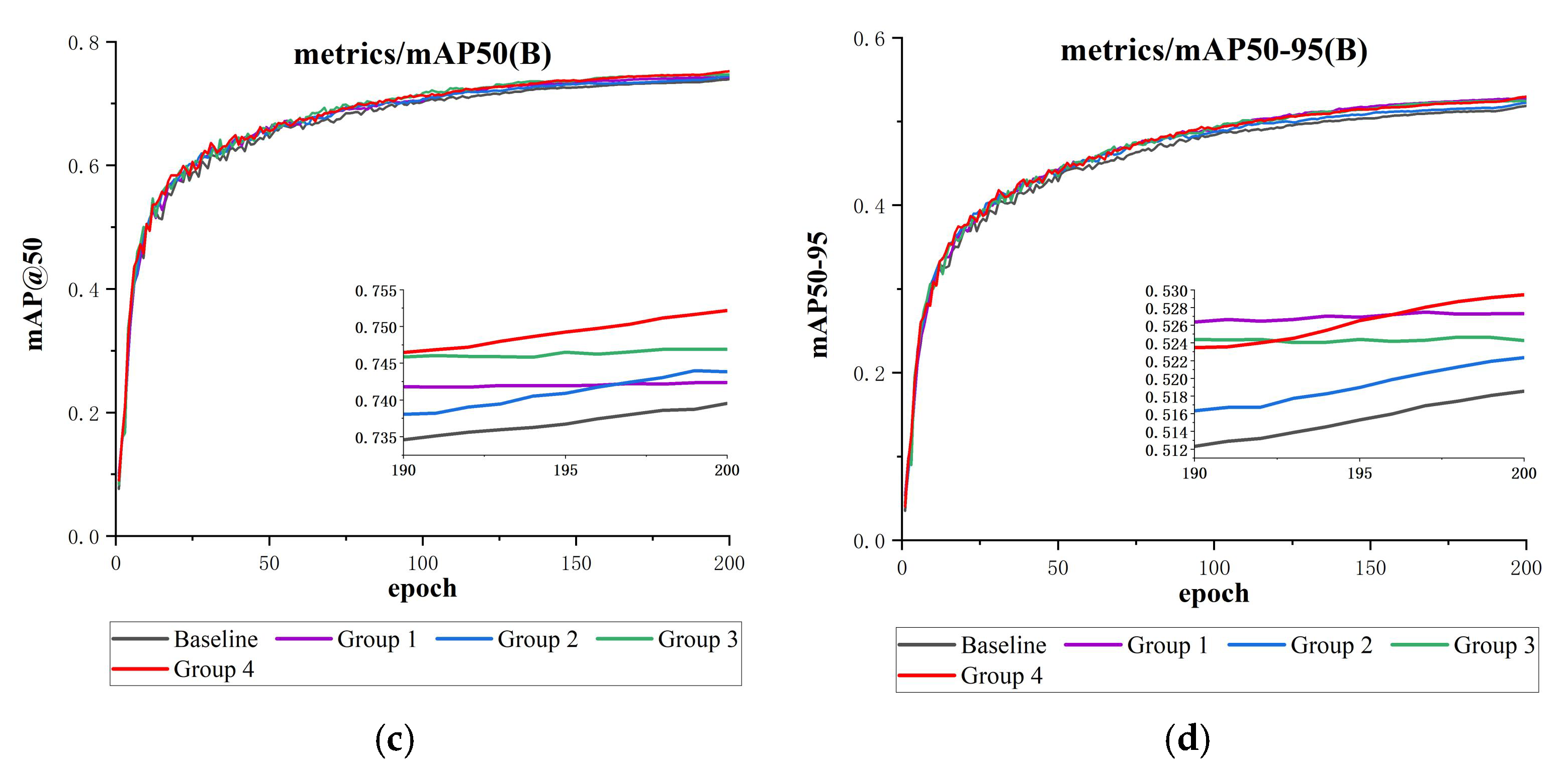
Figure 15.
This is a loss function comparison results plot (containing detailed subgraphs for 190–200 epochs): (a) precision comparison, (b) recall comparison, (c) mAP@50 comparison, and (d) mAP@50-95 comparison.
Figure 15.
This is a loss function comparison results plot (containing detailed subgraphs for 190–200 epochs): (a) precision comparison, (b) recall comparison, (c) mAP@50 comparison, and (d) mAP@50-95 comparison.
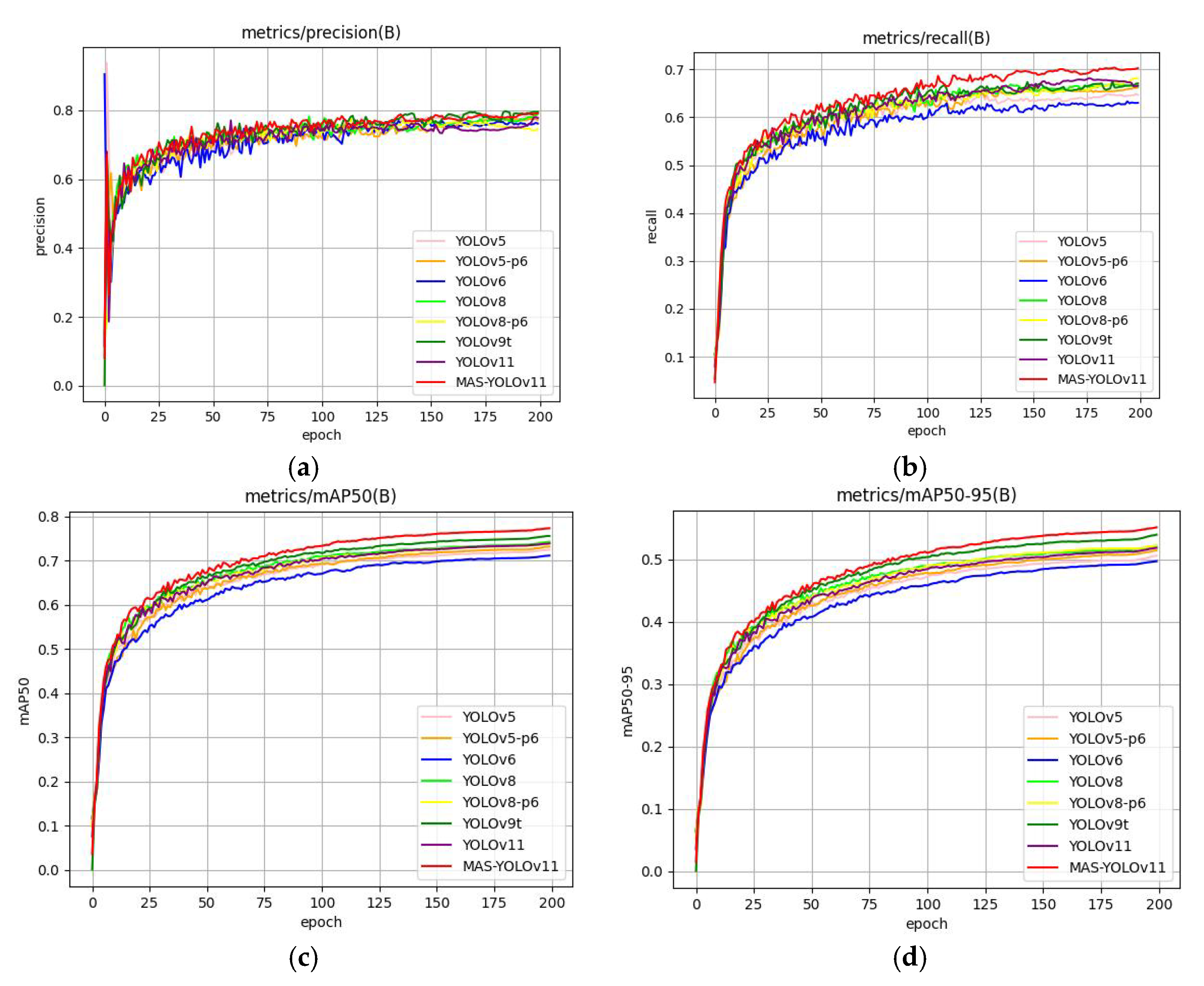
Figure 16.
This is a diagram of a model comparison experimental results chart: (a) precision comparison, (b) recall comparison, (c) mAP@50 comparison, and (d) mAP@50-95 comparison.
Figure 16.
This is a diagram of a model comparison experimental results chart: (a) precision comparison, (b) recall comparison, (c) mAP@50 comparison, and (d) mAP@50-95 comparison.
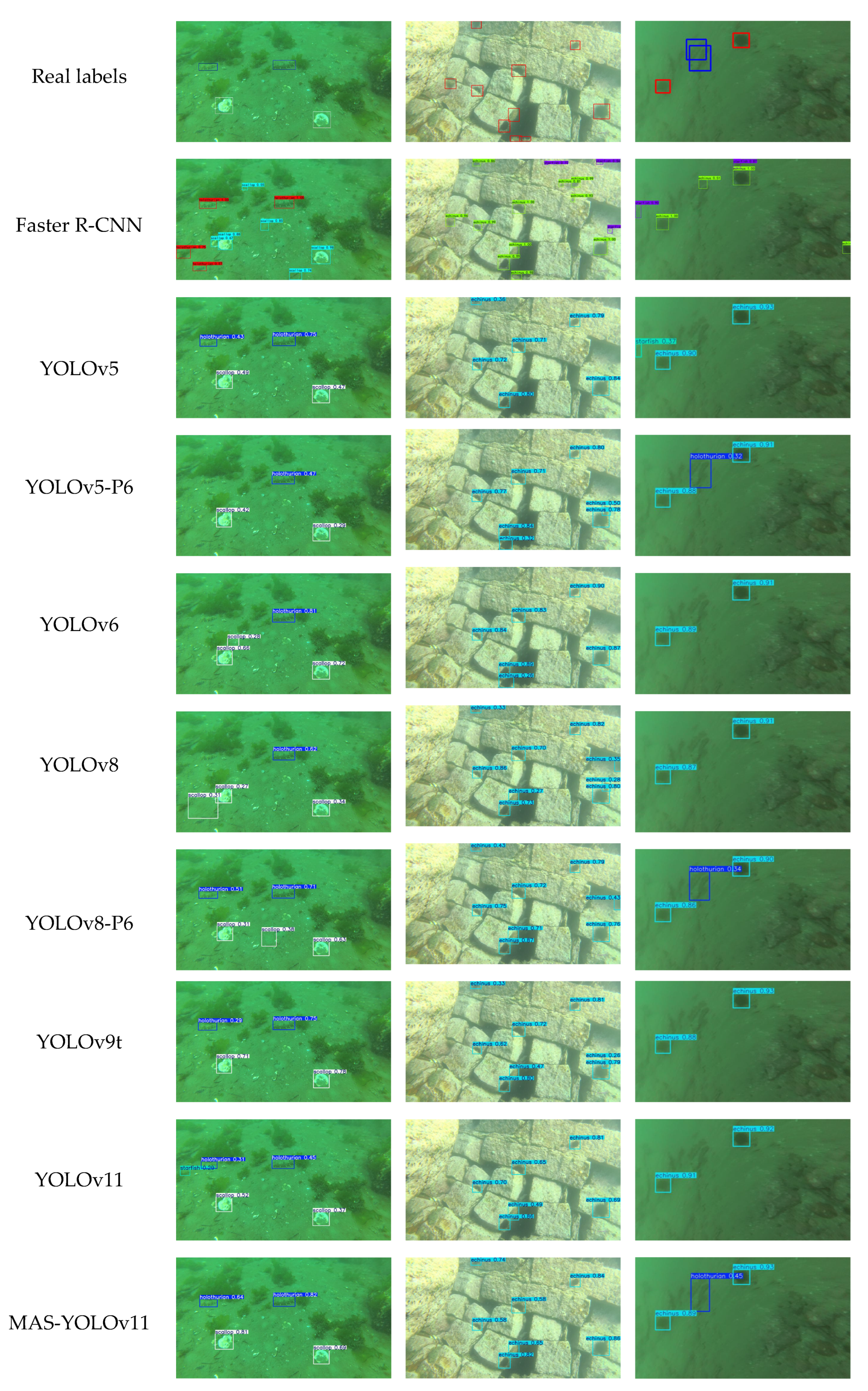
Figure 17.
This is a comparison of the detection results of each model.
Figure 17.
This is a comparison of the detection results of each model.
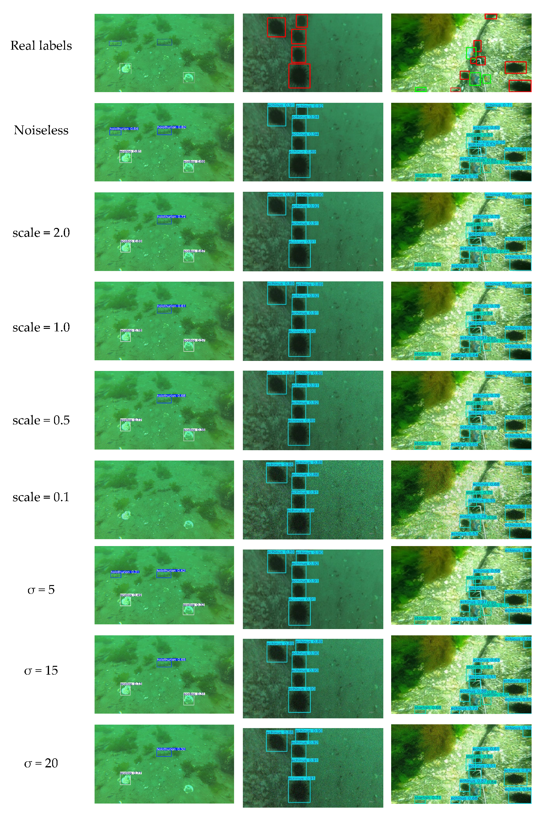
Figure 18.
Test results at different noise intensities.
Figure 18.
Test results at different noise intensities.
Table 1.
Experimental environment parameters table.
Table 1.
Experimental environment parameters table.
| Training Parameters | Values |
|---|
| Learning rate | 0.01 |
| Momentum | 0.937 |
| Weight decay | 0.0005 |
| Batch size | 16 |
| Optimizer | SGD |
| Image size | 640 × 640 |
| Epoch | 200 |
| Patience | 20 |
Table 2.
Comparison of the results before and after the improvement of the YOLOv11 model (unit: %). Bold font indicates the best performance values under the same evaluation metric.
Table 2.
Comparison of the results before and after the improvement of the YOLOv11 model (unit: %). Bold font indicates the best performance values under the same evaluation metric.
| Net | AP-Ho | AP-Ec | AP-Sc | AP-St | P | R | F1 | mAP@50 | mAP@50-95 |
|---|
| YOLOv11 | 57.9 | 90.6 | 59.3 | 88 | 77.8 | 66.6 | 71 | 73.9 | 51.8 |
| MAS-YOLOv11 | 64 | 91.1 | 65.5 | 88.7 | 78.8 | 70.3 | 74 | 77.4 | 55.1 |
Table 3.
Overall evaluation index of the MAS-YOLOv11 model in the RUOD dataset (unit: %).
Table 3.
Overall evaluation index of the MAS-YOLOv11 model in the RUOD dataset (unit: %).
| Net | P | R | F1 | mAP@50 | mAP@50-95 |
|---|
| MAS-YOLOv11 | 79.2 | 69 | 73 | 76 | 50.9 |
Table 4.
The detection accuracy of each category of RUOD (unit: %). The categories in the table, from left to right, are holothurian, echinus, scallop, starfish, fish, corals, divers, squid, turtles, and jellyfish.
Table 4.
The detection accuracy of each category of RUOD (unit: %). The categories in the table, from left to right, are holothurian, echinus, scallop, starfish, fish, corals, divers, squid, turtles, and jellyfish.
| Net | AP-Ho | AP-Ec | AP-Sc | AP-St | AP-Fi | AP-Co | AP-Di | AP-Cu | AP-Tu | AP-Je |
|---|
| MAS-YOLOv11 | 65 | 82.6 | 66.5 | 83.9 | 61.7 | 62.5 | 87.3 | 92.5 | 92.7 | 65.3 |
Table 5.
Ablation test results, where “√” indicates the module is included (unit: %). Bold font indicates the best performance values under the same evaluation metric.
Table 5.
Ablation test results, where “√” indicates the module is included (unit: %). Bold font indicates the best performance values under the same evaluation metric.
| Net | C2PSA_MSDA | ASFFHead | Slide Loss | P | R | mAP@50 | mAP@50-95 | Parameter/M | FPS |
|---|
| 1 | | | | 77.8 | 66.6 | 73.9 | 51.8 | 2.59 | 109.3 |
| 2 | √ | | | 77.1 | 66.8 | 74 | 52.1 | 2.60 | 96 |
| 3 | | √ | | 80 | 68.1 | 76.4 | 54.5 | 3.96 | 79.5 |
| 4 | | | √ | 76 | 68.2 | 75.2 | 52.9 | 2.59 | 107.4 |
| 5 | √ | √ | | 79.5 | 69.8 | 77.1 | 55.4 | 2.59 | 71.9 |
| 6 | √ | √ | √ | 78.8 | 70.3 | 77.4 | 55.1 | 2.59 | 74.4 |
Table 6.
Experimental setup for attention mechanism comparison.
Table 6.
Experimental setup for attention mechanism comparison.
| Experimental Group | Combination of Modules | Improvement Points |
|---|
| Baseline | ASFFHead | Control group |
| Group 1 | DAT + ASFFHead | Improve the adaptability of the model to the deformation target |
| Group 2 | EMA + ASFFHead | Optimize cross-channel interaction and improve the utilization of multi-scale features. |
| Group 3 | iEMA + ASFFHead | Enhance feature fusion efficiency and reduce computational redundancy |
| Group 4 | MLCA + ASFFHead | Balance the computational cost with feature discrimination |
| Group 5 | MSDA + ASFFHead | Combined with dynamic convolution, it strengthens the target perception of complex scenes. |
Table 7.
Comparative results of attention mechanism (unit: %). Bold font indicates the best performance values under the same evaluation metric.
Table 7.
Comparative results of attention mechanism (unit: %). Bold font indicates the best performance values under the same evaluation metric.
| Experimental Group | P | R | mAP@50 | mAP@50-95 | Parameter/M | FPS |
|---|
| Baseline | 80 | 68.1 | 76.4 | 54.5 | 3.96 | 79.5 |
| Group 1 | 79.5 | 68.9 | 76.7 | 54.5 | 3.99 | 76.2 |
| Group 2 | 80.8 | 68.3 | 76.8 | 55 | 3.91 | 80.3 |
| Group 3 | 77.9 | 67.1 | 74.9 | 53.1 | 3.93 | 78.3 |
| Group 4 | 77.9 | 67.9 | 75.5 | 53.9 | 3.91 | 81.2 |
| Group 5 | 79.5 | 69.8 | 77.1 | 55.4 | 3.98 | 71.9 |
Table 8.
Experimental setup for loss function comparison.
Table 8.
Experimental setup for loss function comparison.
| Experimental Group | Classification Loss | Localization Loss | Improvement Points |
|---|
| Baseline | BCE | DFL + CIoU | Control group |
| Group 1 | BCE | DFL + SIoU | Improved orientation sensitivity for regression boxes |
| Group 2 | BCE | DFL + ShapeIoU | Introduced shape-adaptive weighting |
| Group 3 | Focaler Loss | DFL + CIoU | Dynamically focus on difficult samples |
| Group 4 | Slide Loss | DFL + CIoU | Slide to adjust the weights between samples |
Table 9.
Comparison of loss functions (unit: %). Bold font indicates the best performance values under the same evaluation metric.
Table 9.
Comparison of loss functions (unit: %). Bold font indicates the best performance values under the same evaluation metric.
| Experimental Group | P | R | mAP@50 | mAP@50-95 |
|---|
| Baseline | 77.8 | 66.6 | 73.9 | 51.8 |
| Group 1 | 75.9 | 68.1 | 74.2 | 52.7 |
| Group 2 | 77.7 | 67.5 | 74.4 | 52.2 |
| Group 3 | 77.4 | 67.9 | 74.7 | 52.4 |
| Group 4 | 76.1 | 68.3 | 75.2 | 52.9 |
Table 10.
This is a model comparison results table (unit: %). Bold font indicates the best performance values under the same evaluation metric.
Table 10.
This is a model comparison results table (unit: %). Bold font indicates the best performance values under the same evaluation metric.
| Net | P | R | mAP@50 | mAP@50-95 | Parameter/M | FLOPs/G | FPS |
|---|
| Faster R-CNN | 53.7 | 56.4 | 62.9 | 37.3 | 60.13 | 82.7 | 37.2 |
| YOLOv5 | 77.7 | 64.9 | 72.5 | 50.6 | 2.19 | 5.9 | 131.8 |
| YOLOv5-P6 | 77.3 | 66.3 | 73.3 | 51.5 | 3.69 | 6.0 | 100.7 |
| YOLOv6 | 76.5 | 62.9 | 71.2 | 49.7 | 4.16 | 11.6 | 158.5 |
| YOLOv8 | 79.4 | 66.5 | 74.3 | 52.1 | 2.69 | 6.9 | 133.7 |
| YOLOv8-P6 | 74.4 | 68.2 | 73.9 | 52.2 | 4.34 | 6.9 | 112.2 |
| YOLOv9t | 79.4 | 67.1 | 75.6 | 54 | 1.77 | 6.7 | 61.4 |
| YOLOv11 | 77.8 | 66.6 | 73.9 | 51.8 | 2.59 | 6.4 | 109.3 |
| MAS-YOLOv11 | 78.8 | 70.3 | 77.4 | 55.1 | 3.98 | 8.6 | 74.4 |
Table 11.
Poisson noise test results (unit: %).
Table 11.
Poisson noise test results (unit: %).
| Scale Value | Noise Intensity | P | R | mAP@50 | mAP@50-95 |
|---|
| 0 | None | 78.8 | 70.3 | 77.4 | 55.1 |
| 2.0 | Extremely weak | 73.5 | 56.3 | 63.2 | 42.2 |
| 1.5 | Weak | 72.3 | 51.4 | 58.2 | 38.7 |
| 1.0 | Natural Poisson | 68.0 | 44.3 | 50.2 | 32.8 |
| 0.5 | Medium | 59.2 | 31.6 | 35.7 | 23.0 |
| 0.1 | Strong | 56.3 | 11.3 | 17.7 | 10.7 |
Table 12.
Gaussian noise test results (unit: %).
Table 12.
Gaussian noise test results (unit: %).
| Scale Value | Noise Intensity | P | R | mAP@50 | mAP@50-95 |
|---|
| 0 | None | 78.8 | 70.3 | 77.4 | 55.1 |
| 5 | Extremely weak | 77.1 | 65.3 | 72.8 | 50.3 |
| 10 | Mild | 71.5 | 46.6 | 52.8 | 34.7 |
| 15 | Medium | 60.2 | 31.4 | 35.7 | 22.8 |
| 20 | Strong | 52.5 | 21.4 | 25.7 | 16.1 |


