1. Introduction
In the context of Industry 4.0 [
1] and initiatives like “Made in China 2025” [
2], the digitalization, networking, and intellectualization of Industrial Control Systems (ICSs) [
3,
4] have increased significantly. This transformation brings both opportunities and challenges, especially with the growing number of interconnected devices in ICSs, which exposes systems to greater risks of security threats due to vulnerable interfaces and potential breaches [
5,
6]. Advanced anomaly detection mechanisms, leveraging deep learning methods, aim to improve ICS security and have made substantial progress. However, these mechanisms are primarily designed for large-scale factories [
7,
8]. In contrast, small and medium-sized factories face unique challenges due to limited computational resources. These factories typically have a moderate amount of computing power, including CPUs and GPUs, but they lack the high-performance infrastructure needed to train complex and computationally expensive neural networks [
9]. Consequently, there is a demand for lightweight anomaly detection mechanisms that require fewer parameters, faster training times, and shorter deployment periods. Moreover, the dynamic nature of production lines and frequent changes in data patterns make it difficult for existing solutions to adapt quickly to new data features. As a result, retraining such systems can become impractical and resource-intensive. Small and medium enterprises are a noteworthy driver of economic development [
10], being vital to most economies across the world, particularly in developing and emerging nations [
11,
12]. Thus, there is a pressing need for lightweight, efficient, and adaptive anomaly detection mechanisms that address security risks while accommodating the resource constraints of small and medium-sized factories.
Current anomaly detection algorithms for multivariate time series data can be categorized into three types: The first type comprises reconstruction-based models [
8], such as autoencoder (AE) [
13] and Generative Adversarial Networks (GANs) [
14]. AE models are prone to overfitting, especially when dealing with noisy data, which results in reduced accuracy [
15]. GANs, due to their adversarial nature, often suffer from instability, making them less reliable for consistent performance [
16]. These methods, while useful, struggle to balance high computational precision with stability and efficiency, which is a critical need for real-time anomaly detection in small and medium-sized factories. The second type involves graph networks [
17], which convert multivariate time series into graph structures to capture complex dependencies between dimensions and time points. Although graph networks are effective in modeling intricate relationships, they are computationally expensive due to the reliance on complex matrix operations and high-dimensional data representations. This computational overhead makes them impractical for small and medium-sized factories, where limited resources cannot afford such high computational costs. In this case, the high computational overhead compromises both efficiency and adaptability, further straining the system’s ability to operate in dynamic factory environments. The third type consists of prediction-based models [
18], which apply predictive modeling to forecast time series data. Anomalies are detected by comparing real-time observations against predicted values. However, many prediction-based models use fixed models, which cannot adapt to changes in the data over time. This lack of adaptability leads to frequent retraining, which is computationally demanding and inefficient, particularly in environments with limited resources. These models struggle to balance high prediction accuracy and adaptive learning, resulting in excessive computational overhead and poor resource utilization. Simple reconstruction-based algorithms suffer from low accuracy and instability, graph networks algorithms face high computational demands, and prediction-based models lack adaptability and incur high retraining costs. In brief, existing anomaly detection algorithms struggle to balance the four key requirements: high stability, high computational precision, low computational cost, and strong adaptability. Moreover, many ICS sensors themselves operate under severe resource constraints, often limited to just a few kilobytes of SRAM and flash memory. For example, embedding a block-based Kalman-filter model in an Arduino Uno consumes 1.3 kB of its 2 kB SRAM and 13.5 kB of its 32 kB flash memory [
19]. Consequently, minimizing on-sensor memory footprint and computational load must be treated as an additional, fifth design criterion for any real-time anomaly detector in industrial settings.
To address these challenges, we proposed DBN-BAAE, a new lightweight anomaly detection mechanism that combines deep belief networks (DBNs) [
20] with a boosting adversarial autoencoder (BAAE). This mechanism reduces computational overhead, enhances training stability, and achieves high detection accuracy and improved adaptability with faster anomaly detection, specifically designed for small and medium-sized industrial environments with limited resources. Firstly, the instability during training is addressed by leveraging an optimized DBN for pre-training. The DBN provides the autoencoder with a good initialization, ensuring more stable training. Secondly, to address the high computational overhead of graph network algorithms, we introduced a lightweight BAAE that reduces computational overhead while maintaining effectiveness. By optimizing the architecture and reducing the complexity of the mechanism, we ensure faster anomaly detection with lower resource consumption. Thirdly, to address the challenge of detecting anomalies that closely resemble normal data and improving detection accuracy, we introduced an enhanced boosting adversarial encoder based on ensemble learning [
21]. This approach enhances data feature extraction and amplifies reconstruction errors, enabling the mechanism to capture anomalies in complex ICS data more effectively, thus improving detection accuracy. Lastly, to solve the issue of model retraining due to changes in production lines in small and medium-sized factories (lack of adaptability), we proposed using dynamic thresholds to adapt to new data patterns, providing adaptability and reducing computational overhead for model retraining. Furthermore, we conducted comprehensive comparison experiments to evaluate detection accuracy and training speed. Experiments validate that the mechanism attains an F1 score of 0.82, outperforming the best baseline algorithm, and improves training by 2.2 times.
The main contributions of this work are as follows:
DBN-BAAE framework: This work introduces DBN-BAAE, a novel lightweight anomaly detection mechanism based on boosting adversarial learning for ICS. The proposed DBN-BAAE offers not only better stability, improved training speed, but also high anomaly detection accuracy, low computational overhead, and adaptability, making it especially meet the needs of small and medium-sized factories.
Notable performance gains: On benchmark data, DBN-BAAE achieves an F1 of 0.82, higher than all compared baseline algorithms, trains 2.2 times faster, and improves the detection time by 27% compared with the best-performing baseline algorithm.
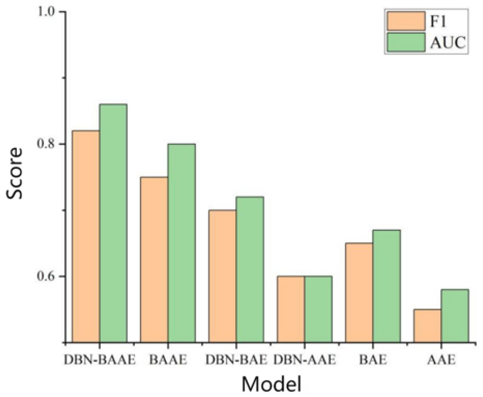
Fusion-driven gains: Ablation studies reveal that our fusion mechanism yields the best anomaly detection performance.
The subsequent sections are organized as follows:
Section 2 discusses methods for detecting unsupervised [
22] anomalies in multivariate time series [
23].
Section 3 presents the motivation of our work.
Section 4 elaborates on our proposed DBN-BAAE mechanism,
Section 5 and
Section 6 present the experimental details and showcase the state-of-the-art performance of our mechanism, respectively.
2. Related Work
This section reviews anomaly detection methods for multivariate time series, categorizing them into reconstruction-based, graph network-based, and prediction-based approaches. Reconstruction-based approaches detect anomalies by measuring reconstruction error. Graph network-based methods build relational graphs over variables. Prediction-based models forecast future values and flag deviations. To better reflect the strengths and weaknesses of each category, we explicitly compare them in terms of detection accuracy, training stability, computational cost, and adaptability: reconstruction-based models provide interpretability but often overfit noisy data; graph network-based methods capture inter-series dependencies with high precision yet incur heavy memory use and slow convergence; prediction-based models train quickly and support online forecasting but struggle with long-range dependencies and adapting to shifting data patterns.
Li et al. [
24] introduced a hidden Markov model that transforms multivariate anomaly detection into univariate anomaly detection. However, this method results in ineffective detection of anomalies. Tuli et al. [
25] proposed a deep transformer-based model TranAD using Model-Agnostic Meta-Learning (MAML) for fast training and large sequence processing, but the detection accuracy needs improvement. Lee et al. [
26] used a lightweight Long Short-Term Memory (LSTM) [
27] model based on historical data points to predict abnormal data, but the detection accuracy needed improvement. These methods have scope for improvement in detection accuracy and exhibit training instability, which limits their effectiveness in reliably identifying anomalies.
Su et al. [
28] introduced a stochastic recurrent neural network model OmniAnomaly which combines Gated Recurrent Unit (GRU) [
29] and Variational Autoencoder (VAE) [
30], using the reconstruction probability to make anomaly judgments, but the computational complexity of the algorithm is high. Li et al. [
31] devised a GAN-based method using a dilated convolutional transformer (DCT-GAN), though it suffers from a time-consuming process. Yu et al. [
32] designed the maximum information coefficient attention graph network (MAG), which combines a graph neural network, embedding vectors, and LSTM, but computational efficiency may need optimization. Zhao et al. [
33] used graph attention networks to extract connections in multivariate time series, but the convergence time is relatively high. These models, although effective, have high computational costs, which limit their feasibility for anomaly detection tasks in resource-constrained environments.
Park et al. [
34] combined LSTM with a VAE for anomaly detection, using reconstruction error and probability but with limited adaptability. Munir et al. [
35] proposed DeepAnT, a fixed Convolutional Neural Network (CNN) [
36] that predicts future values, but this model lacks adaptability to changing patterns in the ICS data. Park et al. [
37] proposed a model combining CNN with autoencoders. Pietroń et al. [
38] optimized automatic encoders using genetic operators to reduce training data and improve accuracy without sacrificing speed, yet the model’s adaptability could be enhanced to handle dynamic data patterns better. These methods struggle to adapt to changing data patterns, limiting their applicability in environments with evolving anomaly characteristics.
Despite these advances, no existing method simultaneously delivers high accuracy, robust stability, low computational overhead, and adaptability, particularly under the resource constraints of small and medium-sized factories. This gap motivates our proposed DBN-BAAE model, which combines boosting adversarial learning with a compact architecture to achieve fast convergence, low resource use, and reliable anomaly detection across evolving data patterns. See
Table 1.
4. Method
4.1. Overview
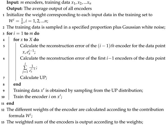
The proposed deep belief network-based boosting adversarial autoencoder, termed DBN-BAAE, is a novel lightweight anomaly detection mechanism for ICSs based on a boosting adversarial autoencoder, as shown in
Figure 1. It consists of five main steps, with the dashed line highlighting the innovations of this work. Unlike typical anomaly detection methods, this work introduces a DBN pre-training step before neural network training to enhance algorithm stability. Additionally, a two-stage training process with a boosting encoder and adversarial decoder is proposed, simplifying the structure and improving detection accuracy. Finally, during the anomaly detection phase, the Streaming Peaks Over Threshold (SPOT) [
39] threshold is dynamically updated based on the test data, enhancing adaptability.
The first step, data pre-processing, involves normalizing time series data from factory sensors and applying the sliding window technique [
40] to create time series windows for easier training and detection.
The second step, enhanced DBN pre-training, involves maximizing stability by pre-training with an enhanced DBN model to provide a good initial state for the autoencoder. This enables the autoencoder to find a better minimum during training, enhancing training stability.
The third step, enhanced boosting encoder training, is required in order to improve the reconstruction ability of the autoencoder while maintaining its simplicity. The enhanced boosting encoder utilizes the weight matrices learned during the DBN pre-training as a starting point to construct m deep autoencoders and two decoders. These components are trained iteratively using ensemble learning techniques, allowing the model to learn multiple representations of the data, thereby improving its overall performance and robustness.
The fourth step, adversarial decoder training, involves amplifying data reconstruction errors using an adversarial approach with Decoder1 as the generator and Decoder2 as the discriminator.
The fifth step, dynamic threshold for anomaly detection, improves the model’s adaptability. The dynamic threshold is proposed based on test data anomalies, which are updated according to the results.
4.2. Enhanced DBN Pre-Training
In this subsection, we discuss the second step of the proposed DBN-BAAE mechanism, enhanced DBN pre-training. To improve feature extraction and stabilize convergence of autoencoders, we propose using an enhanced DBN for pre-training. A DBN is a multi-layer neural network model that learns feature representations layer-by-layer using a restricted Boltzmann machine (RBM) [
41] with multiple hidden layers. The pre-training process initializes network parameters layer-by-layer through greedy unsupervised training [
42], making optimization easier. This process, using an RBM, employs the Contrastive Divergence (CD) algorithm [
43].
In the first step, initializing network parameters, we set weights and biases for each layer. In DBN, the first layer is the visual layer, the last is the output layer, and the intermediate layers are hidden layers.
In the second step, training the first RBM, we feed data into the first layer’s RBM, perform several CD iterations, and update the weights and biases.
In the third step, we train subsequent RBMs. Using the output of the previous layer as input for the current layer, we perform multiple CD iterations, and update weights and biases.
By using DBN pre-training, the autoencoder is effectively guided toward a better local minimum in the parameter space. This is because each RBM layer refines the feature representations, reducing the likelihood of getting stuck in poor local minima when the autoencoder is subsequently fine-tuned.
4.2.1. Improved Parameter Initialization Method
To achieve rapid convergence and ensure training stability in a DBN, we propose a combined approach of random initialization and greedy layer-by-layer initialization. Proper parameter initialization, including weight matrices, bias vectors, learning rate, number of network layers, and nodes, is essential for improving convergence time and stability.
Random initialization provides each layer’s weights and biases with random values before training. While random initialization is quick, it can lead to fluctuations during early training steps, thereby slowing down convergence. To mitigate the drawbacks of purely random initialization, we apply greedy layer-by-layer training using RBMs. Specifically, we train each RBM on top of the output (hidden representation) of the previous RBM. This approach stabilizes the parameter space by progressively learning meaningful features, ensuring that each subsequent layer starts from a better-informed initialization rather than purely random values.
4.2.2. Improved Adaptive Learning Rate Approach
To efficiently approximate the probability distribution of real data in RBM training, we use the Contrastive Divergence-
K (CD-
K) algorithm instead of stochastic gradient descent alone. CD-
K, a Markov Chain Monte Carlo (MCMC) [
44] sampling algorithm, starts by selecting an initial state and then simulates the Markov process through cyclic sampling. This approach helps achieve a smooth distribution, overcoming the limitations of requiring numerous Gibbs sampling cycles.
Traditional CD-K uses a fixed learning rate, which remains constant regardless of parameter update direction. In contrast, adaptive learning rates adjust dynamically based on update direction, helping RBMs avoid local minima and improving performance. However, previous global adaptive learning methods applied a uniform learning rate across all DBN levels, which may not optimize all RBMs effectively.
Fine-Grained Adaptive Learning Rate
We propose an enhanced fine-grained adaptive learning rate to accelerate RBM training:
where
and
are two hyperparameters (
is the increment factor and
is the decrement factor). Here,
denotes the initial learning rate, which controls the magnitude of weight updates before adaptation and
and
are consecutive weight updates. These updates are computed as
where
k is the number of Gibbs samples and
denotes the average output of Gibbs sampling. In practice,
is obtained by computing the expectation of the product
under the empirical data distribution, whereas
is the corresponding expectation under the model distribution after
k steps of Gibbs sampling. At each training iteration, we compute
(for the current update) and
(for the previous update) for each layer. The DBN then checks the sign of the dot product
to decide whether to increase or decrease the learning rate. If the signs of these updates are the same, the learning rate increases to accelerate convergence; otherwise, it decreases to avoid overshooting. This adaptive mechanism is applied individually to each layer, allowing fine-grained control over each RBM’s training.
4.2.3. Evaluation and Stability Analysis
Enhanced DBN pre-training provides the autoencoder with more discriminative initial features. By training RBMs layer-by-layer, the DBN builds a hierarchy of features that guides the autoencoder toward a better local minimum, resulting in more stable and reliable convergence compared to training without DBN pre-training.
To highlight the importance of enhanced DBN pre-training, we compare autoencoders with and without DBN pre-training. Using the dataset from the last day, we visualize the data after applying Principal Component Analysis (PCA) [
45] to extract two principal components during autoencoder training, shown in 2D plots in
Figure 2. The blue points represent the input data projections, and the red points represent the feature projections learned by the autoencoder.
Without DBN pre-training:
Figure 2a,b show the feature projections at the start and end of training. Although there is some clustering in the red points, the spread is still relatively large in
Figure 2b, indicating higher variance and less stable convergence.
With DBN pre-training:
Figure 2c,d show that even at the start of training (
Figure 2c), the feature projection (red points) is already more compact and better structured. By the end of training (
Figure 2d), the red points converge to a much denser and more stable cluster.
Comparing
Figure 2c and
Figure 2d demonstrates the stability of our approach: the feature distribution in
Figure 2d remains tight and less scattered, indicating that the model parameters have settled into a stable region with lower reconstruction error. In contrast, without DBN pre-training, the autoencoder’s parameters often oscillate longer before converging, as seen in the relatively dispersed feature distribution of
Figure 2b.
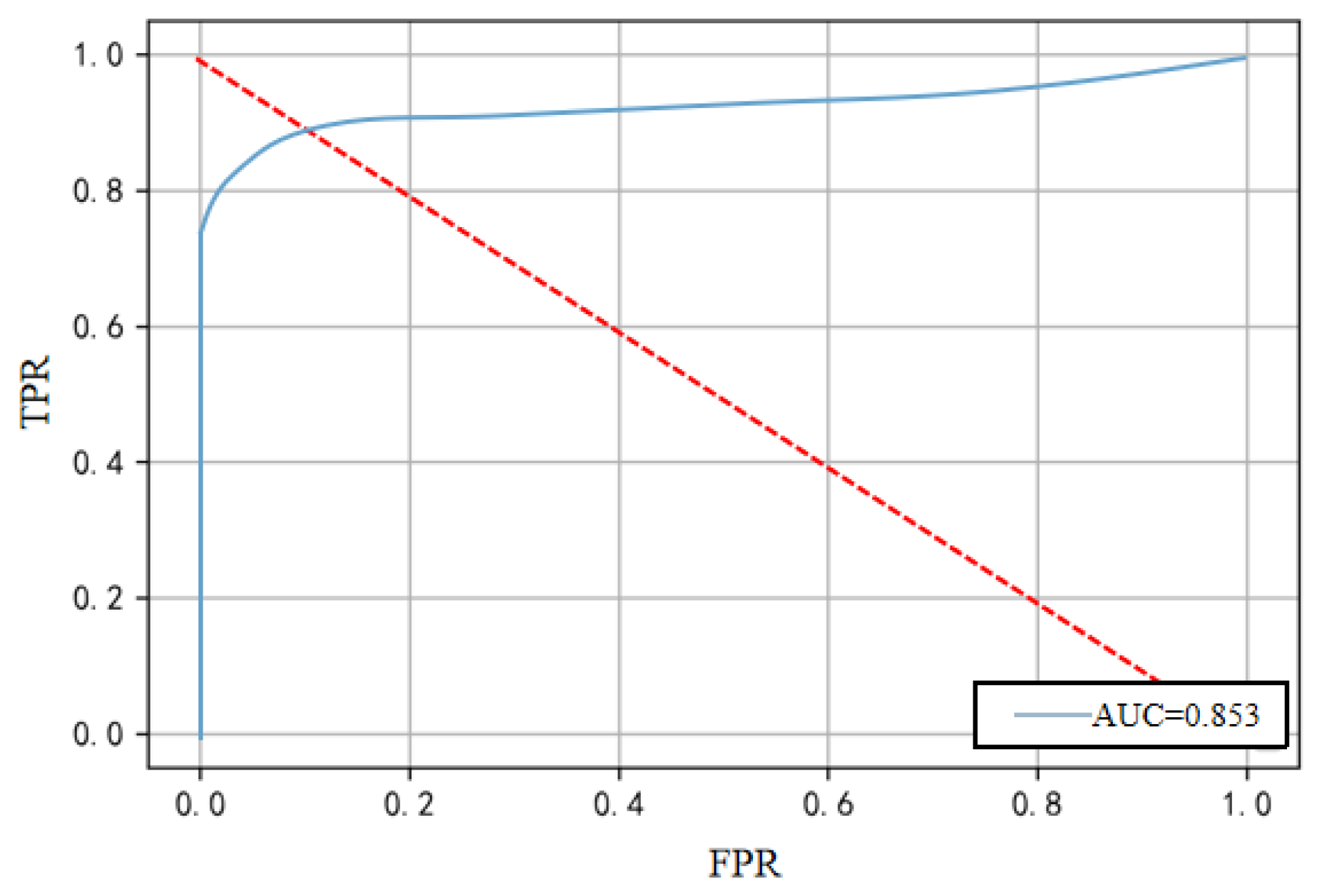
To assess the impact of the extracted features on anomaly detection, we compare the AUC scores of autoencoders with and without DBN pre-training, as shown in
Figure 3. In
Figure 3, the AE-only model experiences sharp AUC declines to around 0.50 in experiments 3, 7 and 10. These performance dips arise from the stochastic nature of weight initialization and from certain noise realizations that can trap a single autoencoder in a suboptimal reconstruction result. Consequently, its ability to distinguish normal from anomalous patterns is affected. The pre-trained model exhibits more stable and consistent performance across multiple experiments, demonstrating that enhanced DBN pre-training improves the overall stability of autoencoder training and its effectiveness for downstream anomaly detection.
4.3. Neural Network Training
In this subsection, we discuss the third step of the proposed DBN-BAAE mechanism, enhanced boosting encoder training, and the fourth step, adversarial decoder training.
Neural network [
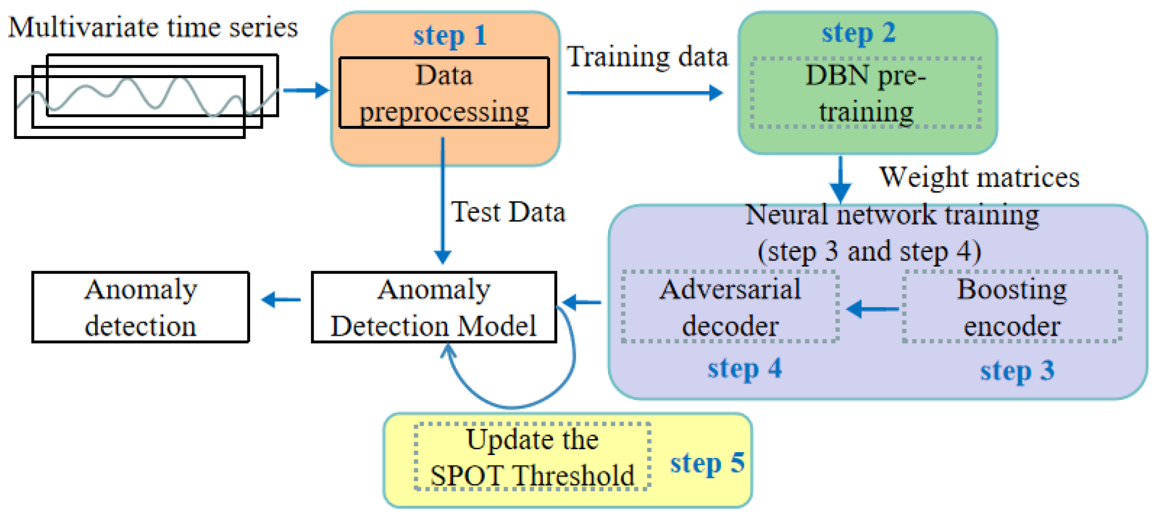
46] training involves two steps, as shown in
Figure 4. First, an enhanced boosting encoder is used. Since simple encoders have limited capability with multidimensional data, multiple integrated encoders are employed to improve feature extraction. This approach also mitigates issues like false outliers and feature loss caused by the mean function in the output. Second, an adversarial decoder structure is introduced. Traditional encoder–decoder models struggle with detecting anomalies close to normal values, reducing accuracy. To address this, adversarial learning is incorporated at the decoder stage, enhancing its ability to distinguish real data and improving detection accuracy. In
Figure 4, the horizontal axis denotes the sequential flow of data: raw input
W to boosted encoder branches to latent code
Z to two-stage adversarial decoding (AE
1 then AE
2).
4.3.1. Enhanced Boosting Encoder Training
Ensemble learning uses multiple decision models instead of a single one to reduce bias and variance in the classifier [
21]. In this algorithm, the encoder layer comprises
m encoders, each maintaining a distribution function of data points to guide the focus of the next encoder. The weight of the distribution function is updated based on the mean square error between the input and the decoder output, as shown in Equation (
4):
the reconstruction error of the data point
x in the (
)th encoder is denoted as
, with a positive hyperparameter
to prevent excessively large weights. Data points with higher reconstruction errors are more likely to be sampled in the next training, allowing further learning. This approach combines multiple autoencoder results, focusing on hard-to-reconstruct data and reducing the risk of overfitting to normal data.
However, during early computation, some data points may have large initial reconstruction errors, which are normal at the initialization stage and not true anomalies. Simple sampling based on reconstruction error can cause the model to repeatedly select these points, leading to overfitting and high false alarm rates on new data. Averaging outputs of multiple autoencoders can also lead to ignoring important contributions from some, reducing detection performance. To address these issues, we introduce an enhanced boosting encoder. To mitigate early false anomalies, we employ weighted sampling that equally focuses on both abnormal and normal samples, thereby enhancing feature learning. Additionally, we refine the weight update formula by incorporating two distinct probability measures to emphasize both normal and abnormal samples. The Normal Probability (
) is designed to prioritize normal samples and is defined in Equation (
5) as
where
is the reconstruction error of sample
x obtained from the
th encoder. This formulation is inversely proportional to the reconstruction error, thereby assigning a higher probability to samples that are easier to reconstruct.
In contrast, the Anomaly Probability (
), introduced in Equation (
6), aims to emphasize abnormal samples by being directly proportional to the reconstruction error:
Here, a higher reconstruction error leads to a higher probability, highlighting samples that are more difficult to reconstruct and are more likely to be anomalies.
It is important to note that while both
and
use a common normalization term (i.e., the sum of the reciprocals of the reconstruction errors), they serve complementary roles in the training process. The Normal Probability (
) focuses on retaining the information of normal samples, whereas the Anomaly Probability (
) increases the model’s attention to potential anomalies. This dual approach helps balance the learning process, preventing overfitting to either normal or abnormal data. By combining these, the update probability (
) for each data point is obtained as
represents the probability of selecting data point
x during the
th training iteration. A training parameter
, close to one, initially emphasizes
over
, focusing on normal samples to prevent underfitting when false outliers are prevalent. As training progresses and false outliers decrease,
decreases while
increases, enabling the model to better fit real outliers. This strategy prevents early underfitting and ensures the model learns challenging samples later, improving robustness and accuracy.
Moreover, instead of a simple average which treats all encoders equally and may dilute specialized features learned by high-performing encoders, we employ a weighted fusion strategy. We define the weight
The fused feature representation is then computed as a convex combination of individual encoder outputs
:
Theoretical justification for this weighted fusion arises from ensemble learning theory [
47], which shows that convex combinations weighted by individual model reliability minimize ensemble variance and bias. By assigning higher weights to encoders with smaller reconstruction errors, the fused representation emphasizes more reliable feature mappings, yielding a richer and more discriminative feature space than uniform averaging or a single autoencoder.
To further enhance feature robustness during detection, a Gaussian noise layer is added before training, as represented by Equation (
10):
where
controls the noise variance. The theoretical benefits of Gaussian noise injection are well documented:
Decision-boundary smoothing. From the Vicinal Risk Minimization perspective [
48], sampling in a local neighborhood around each training example enforces Lipschitz continuity of the learned function, improving generalization to unseen perturbations.
Robust feature learning. In autoencoder-based models, noise injection yields a denoising effect—akin to contractive autoencoders—that promotes stable representations under input variations [
49].
The proposed method involves adding a Gaussian noise layer to the original data
x, where
is the noise vector obtained through Gaussian sampling, and
represents the noise-processed data. The pseudo-code for this procedure is presented in Algorithm 1.
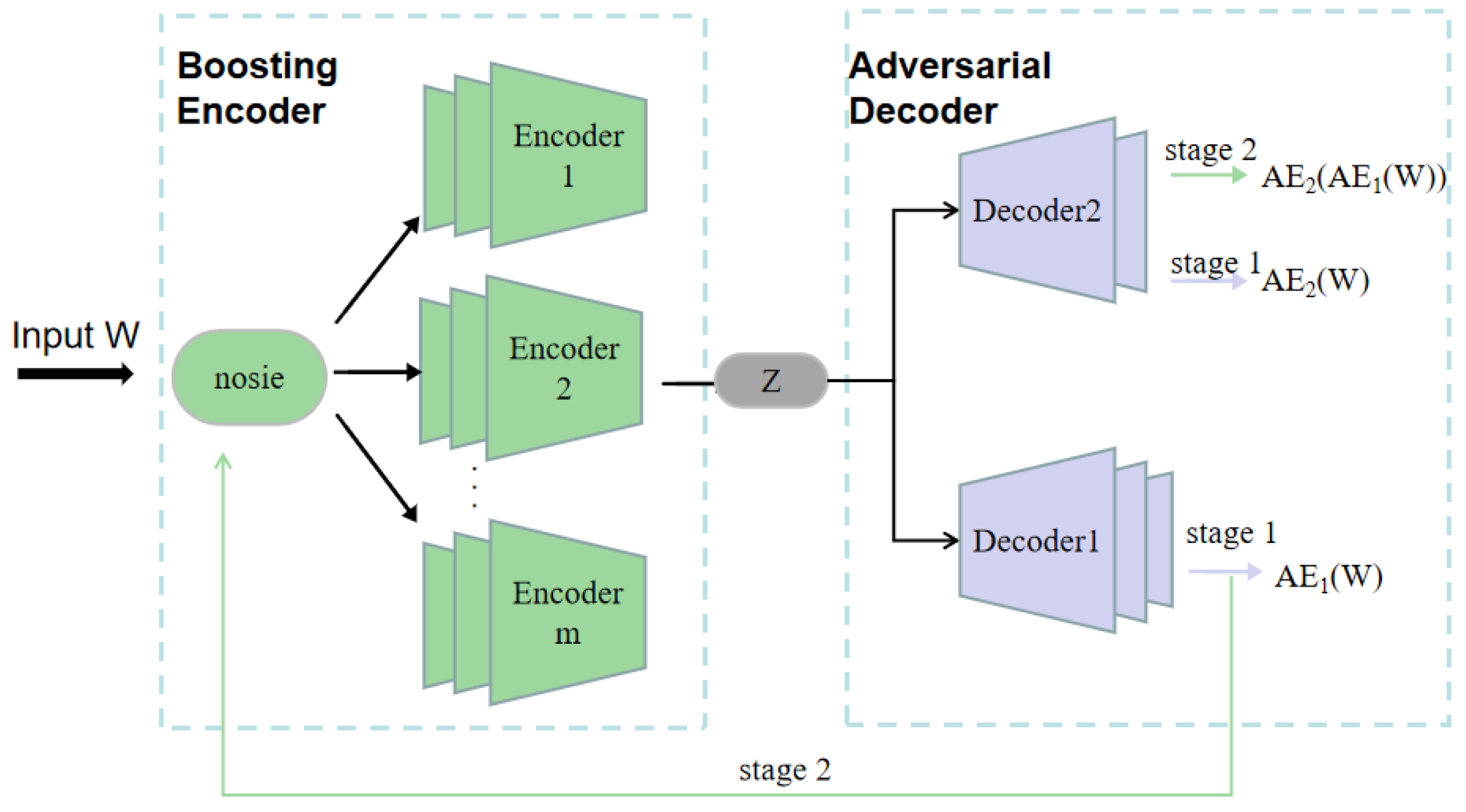
| Algorithm 1: Enhanced boosting encoder training |
![Sensors 25 03249 i001]() |
4.3.2. Adversarial Decoder Training
To highlight the importance of adversarial training, an analysis of data characteristics is conducted. Three representative data dimensions, LIT101, LIT301, and LIT401, are selected from key sensors. Abnormal data from the past four days, including attack points, are depicted in a box diagram (
Figure 5), revealing that these anomalies cluster closely around the median, making them hard to detect. To address this, an adversarial decoder is proposed. This decoder allows
to determine if data generated by
is real during adversarial learning, improving the identification of true anomalies and amplifying reconstruction errors. Inspired by the adversarial training introduced by Goodfellow et al. [
14] with GANs, this method enhances model robustness. GANs, consisting of a generator and a discriminator, are trained against each other: the generator creates fake data, while the discriminator identifies it. Instead of directly using GANs, we apply adversarial training to the existing decoder, allowing for detecting anomalies close to real data while keeping the architecture simple.
A deep
and a shallow
are defined, with
acting as a strong generator that creates realistic data to deceive
. This enables
to detect anomalies that closely resemble normal data, thereby enhancing detection accuracy. During training,
generates fake data to confuse
by minimizing the difference between
and
W. Meanwhile,
is trained to distinguish real data from
’s reconstructions, maximizing the difference with
W. The formulas for each decoder are given in Equations (
11) and (
12):
the overall loss function loss is shown in Equation (
13):
4.3.3. Merging Training
To streamline training and reduce iterations, we propose merging the training of the enhanced boosting encoder and adversarial training into a single stage. In the original two-stage process, the decoder is used in both stages. Specifically,
first minimizes the reconstruction error of input
W and then minimizes the difference between its reconstruction error and
’s. Similarly,
first minimizes the reconstruction error of input
W, then maximizes the difference between its reconstructed data and
’s true data. To simplify and conserve computational resources, we combine these stages into a single iteration with the merged objective functions defined in Equations (
14) and (
15).
During training, a parameter , close to one, is set. Initially, when , the adversarial training weight is nearly zero, giving priority to encoder reconstruction to ensure stability. High early reconstruction loss makes adversarial data inaccurate, so the adversarial loss weight is kept low. As the autoencoder stabilizes and the reconstruction data aligns with the input, adversarial data accuracy improves. Increasing n raises the adversarial loss weight accordingly. An exponential function with a small positive parameter is used for weighting, similar to adaptive parameters in the boosting encoder, optimizing performance across training stages. Intuitively, during the very first iterations, remains close to 1 so the reconstruction loss term dominates (adversarial weight ), which stabilizes gradient updates and allows the autoencoder to learn a smooth manifold of normal data. As training continues, decays to around 0.5, balancing reconstruction and adversarial pressures, which sharpens latent representations around emerging anomaly boundaries. In later iterations, falls below 0.3, so the adversarial loss term dominates (weight > 0.7), driving the model to discriminate subtle anomalies and produce more discriminative features. This gradual shift prevents early training oscillations while ensuring stronger feature extraction in later epochs.
4.4. Dynamic Threshold
In this subsection, we discuss the fifth step of the proposed DBN-BAAE mechanism, the dynamic threshold for anomaly detection.
The multivariate time series deep learning anomaly detection framework includes offline learning and online detection. Offline training produces the anomaly detection model, which is then used for real-time detection. In the online phase, the model calculates anomaly scores for new data and compares them to a threshold. If the score exceeds the threshold, the data is flagged as anomalous. A concise anomaly score formula ensures flexibility across scenarios, and setting the right threshold is crucial: too low triggers false alarms, while too high leads to missed detections. Given the changing data patterns in industrial settings, frequent retraining is impractical, so a dynamically adjustable online threshold is proposed.
To improve model adaptability to changing data and reduce retraining costs, a dynamic threshold method using Extreme Value Theory (EVT) [
39] is introduced. EVT allows inference of extreme events via probability functions without assuming a specific data distribution. According to EVT’s Peak-over-Threshold (POT) theory, exceedances beyond a threshold follow the Generalized Pareto Distribution (GPD). The GPD formula is provided in Equation (
16).
POT defines the extreme value as the probability of a sample exceeding a small value q, with a constant t set at the 98th percentile of the data. Peaks above t but below are considered normal. GPD parameters are estimated using maximum likelihood to determine the threshold for anomaly detection. For real-time detection, the POT algorithm is adapted into the SPOT method, which follows these steps:
- 1.
Initialization: Use POT on the first n values to set the initial threshold .
- 2.
Streaming Detection/Update: For each new score ,
if , mark it as an anomaly and add to set S. If , treat it as normal and update the threshold by re-estimating GPD parameters on the most recent m non-anomalous scores. If , discard from the update to avoid bias from normal baseline noise.
To integrate this threshold into the online anomaly detection stage, we apply a sliding window of size m to the incoming scores and re-fit the GPD only when scores fall between t and the current . This ensures that the threshold adapts smoothly to both abrupt spikes and gradual drifts in the underlying data stream.
Parameter Sensitivity and Validity: We provide the following intuitive guidance on parameter selection, which holds across a variety of industrial time series:
Percentile q: Choosing q closer to 100% makes the threshold more conservative—better at avoiding false positives but possibly slower at catching subtle anomalies. A slightly lower q increases sensitivity to smaller deviations.
Window size m: A larger window smooths out short-term fluctuations but may delay adaptation when the process shifts rapidly. A smaller window enables quicker response at the risk of over-reacting to noise.
Baseline cutoff t: Setting t at the 95th–98th percentile balances the exclusion of routine fluctuations against the inclusion of meaningful extreme values for the update.
Although the model targets complex multidimensional industrial data, it converts this data into univariate anomaly scores through reconstruction and anomaly calculation.
To demonstrate SPOT’s effectiveness, we selected a period of LIT501 sensor data during an attack, characterized by significant outlier fluctuations.
Figure 6 shows the dynamic thresholds and original data using the SPOT algorithm. The SPOT thresholds continuously update with the data stream, effectively detecting anomalies and reducing false positives, making it ideal for real-time factory scenarios and adapting to the changing data in small and medium-sized factory environments.
6. Conclusions
This work proposes an enhanced lightweight anomaly detection mechanism based on boosting adversarial learning, termed the deep belief network-based boosting adversarial autoencoder (DBN-BAAE), which effectively addresses issues related to computational overhead, training stability, training speed, detection accuracy, and adaptive ability in existing models. Specifically, the enhanced lightweight mechanism reduces computational overhead. The improved DBN model effectively addresses the instability of autoencoder training. The proposed model enhances the encoder through ensemble learning and amplifies the decoder’s reconstruction error through adversarial techniques, significantly improving anomaly detection accuracy while maintaining fast training speed. Additionally, a dynamic threshold method is introduced to adapt to the dynamic characteristics of factory data, reducing the model retraining costs. These features make them ideally suitable for small and medium-sized factories with constrained resources, offering significant advantages in terms of overhead, stability, accuracy, and adaptability. Experimental results demonstrate that the model achieves an F1 score of 0.82 and boosts training speed by 2.2 times compared to the best-performing baseline algorithm.
Although the proposed DBN-BAAE mechanism shows promising results, there is potential for further optimization, for instance, employing data dimensionality reduction prior to algorithm training to streamline the network structure and reduce training time. Moreover, in the future, this mechanism should be applied to more datasets as well as real-time environments. Additionally, the dynamic threshold method should be refined to enhance pattern change detection accuracy, and explore the incorporation of online learning frameworks to better adapt to changing factory characteristics.


 ,
, 


