
Development of Non-Invasive Continuous Glucose Prediction Models Using Multi-Modal Wearable Sensors in Free-Living Conditions


Abstract
1. Introduction
- We developed continuous glucose prediction models using data that can be easily acquired with wearables in free-living conditions and investigated the effectiveness of various ML techniques.
- We systematically examined the feature importance and identified the feature categories that contribute most to model performance.
- We benchmarked our models against the state-of-the-art performance (SOAP) and demonstrated the superiority of our models.
2. Materials and Methods
2.1. Dataset
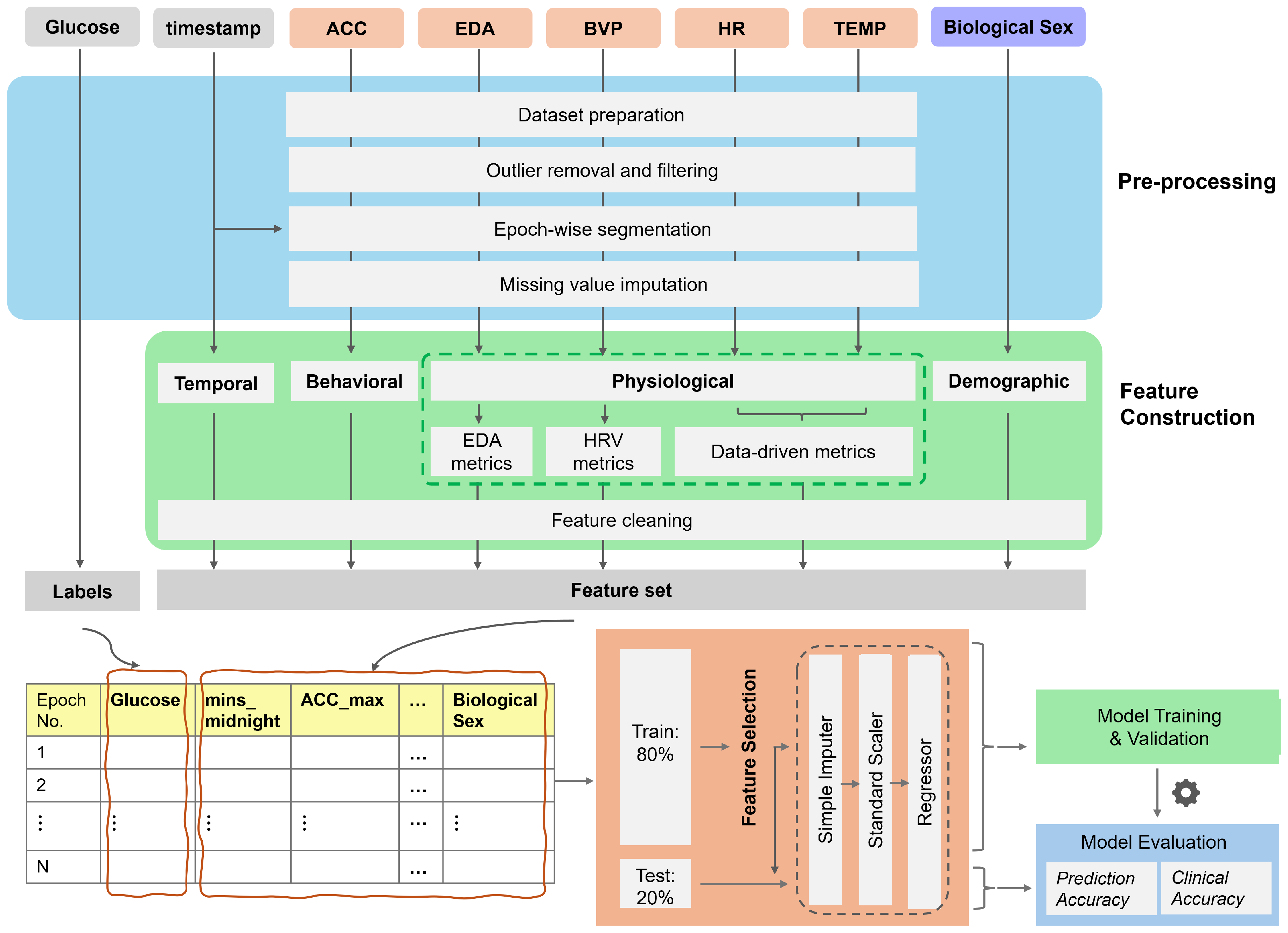
2.2. Preprocessing
- (1)
- Dataset preparationAs the first step, glucose values (mg/dL) recorded from the Dexcom G6 and signals recorded from the Empatica E4 were loaded from the dataset, along with their corresponding timestamps. Samples with missing timestamps were removed, and in cases of duplicate timestamps, only the first occurrence was retained. The tri-axial accelerometer data consisted of acceleration for x, y, and z axes. These values were used to compute the vector magnitude of acceleration (ACC) to represent the overall intensity of movement.
- (2)
- Outlier removal and filteringThis step was tailored to the characteristics of each signal. First, the BVP, EDA, and ACC signals were filtered in the frequency domain following established practices in the literature. The BVP signals were filtered using a fourth-order bandpass filter with a frequency range of 0.5–5 Hz. This frequency band helps remove motion artifacts, baseline wander, and noise due to environmental factors or sensor interferences, such as muscle or electrical noise [43]. For ACC signals, we employed a lowpass filter with a cutoff of 10 Hz to filter out noises introduced by mechanical vibrations, electrical interference, and environmental conditions [44]. The EDA signals were filtered using a low-pass filter, with the cutoff frequency set to 0.5 Hz, as the skin conductance signal is limited to this frequency [45,46]. Next, for each signal, only data within physiologically plausible ranges (HR: 25–240 bpm; sTemp: 30–40 °C; BVP: −500 to 500 (a.u.); EDA: 0.01 to 100 μS; ACC: 0 to 68 ) were retained; other values were deemed invalid and replaced with NaN.
- (3)
- Segmentation into epochsThe signals were synchronized and segmented into epochs using the timestamps from the Dexcom G6 and the Empatica E4. First, the epoch size for each signal was determined using the sampling frequency and the epoch duration. Subsequently, the signals were segmented into epochs and synchronized with the available glucose timestamps. As a result, each epoch represented the 5-minute window preceding a glucose reading. The number of data points in each epoch depended on the sampling rate of the signals. For example, HR data sampled at 1 Hz consisted of 300 data points per epoch, whereas EDA data sampled at 4 Hz consisted of 1200 data points and ACC data sampled at 32 Hz consisted of 9600 data points per epoch, respectively. Epochs with more than 50% missing values in at least one signal were discarded.
- (4)
- Missing value imputationIn the final step, missing values for each signal were imputed based on the epoch-wise distribution. If the distribution was approximately normal (defined as abs(skewness) < 0.5), the mean was used for imputation; otherwise, the median was used.
2.3. Feature Engineering
2.3.1. Feature Construction
- (1)
- Physiological featuresPhysiological features were included to capture changes in autonomic nervous system activity that can be both a response to and a trigger for glucose fluctuations. Physiological features were further divided into the following subcategories: (a) data-driven features, (b) HRV features, and (c) EDA tonic and phasic features.
- (a)
- Data-driven metricsThe data-driven features included time, frequency, and non-linear domain features obtained from physiological signals.Time and frequency domain features are extensively used in biomedical signal processing to capture temporal trends and spectral characteristics of physiological signals [8]. On the other hand, non-linear features have been used in the literature to quantify complexity, irregularity, and deterministic patterns which cannot be adequately captured by solely relying on traditional time- and frequency-domain features [47]. Non-linear features can provide complementary information about underlying signal dynamics and improve model predictions by capturing subtle variations linked to physiological changes and transitions that precede or accompany changes in glucose levels. We constructed non-linear features including recurrence quantification analysis (RQA) features, entropy-based features, fractal features, and complexity-based features using EntropyHub, pyEntrp, Nolds, ordpy, and PyRQA libraries [48,49,50].We constructed 31 time-domain, 14 frequency-domain, and 42 non-linear features (a total of 87 data-driven features) for each of the HR and sTemp signals. Details of these features can be accessed at [51].
- (b)
- HRV metricsFollowing common practice in HRV signal analysis [43], we derived 13 HRV features from the preprocessed BVP signals to capture variations in heart rate and autonomic nervous system activity, such as RMSSD, SDSD, and pNN20.
- (c)
- EDA metricsThe EDA signal is composed of a slow-varying tonic component related to the baseline level of skin conductance and a fast-varying phasic component related to sudden changes in skin conductance in response to stimuli. Following common practice in EDA signal analysis [46], we derived 42 features related to tonic and phasic components of the EDA signal, such as tonic_mean, tonic_std, tonic_energy, phasic_mean, phasic_std, and phasic energy.
- (2)
- Behavioral featuresBehavioral features reflect the effects of lifestyle factors, particularly physical activity and eating, on glucose regulation through modulating insulin sensitivity and glucose uptake. Activity metrics related to the preceding 2-h window for each epoch were derived from the ACC data. Three behavioral features—ACC_2h_min, ACC_2h_max, and ACC_2h_mean—were computed.
- (3)
- Circadian featuresCircadian features represent the influence of circadian rhythm on glucose metabolism, accounting for time-of-day variations in insulin sensitivity and glucose levels. Three circadian features were derived from the timestamps. The first feature, “minutes from midnight”, indicates the time of day. Subsequently, we applied sine and cosine transformations to this feature to account for the cyclical nature of the circadian rhythm.
- (4)
- Demographic featuresDemographic features help account for inter-personal variability in baseline glucose dynamics. The biological sex was used to derive demographic features. One-hot encoding was applied to convert this categorical data into binary. Specifically, ‘male’ was mapped to ‘1’ and ‘female’ was mapped to ‘0’.
2.3.2. Feature Selection
2.4. Model Training and Validation
2.5. Model Testing
3. Results
3.1. Prediction Accuracy
3.1.1. Performance Metrics
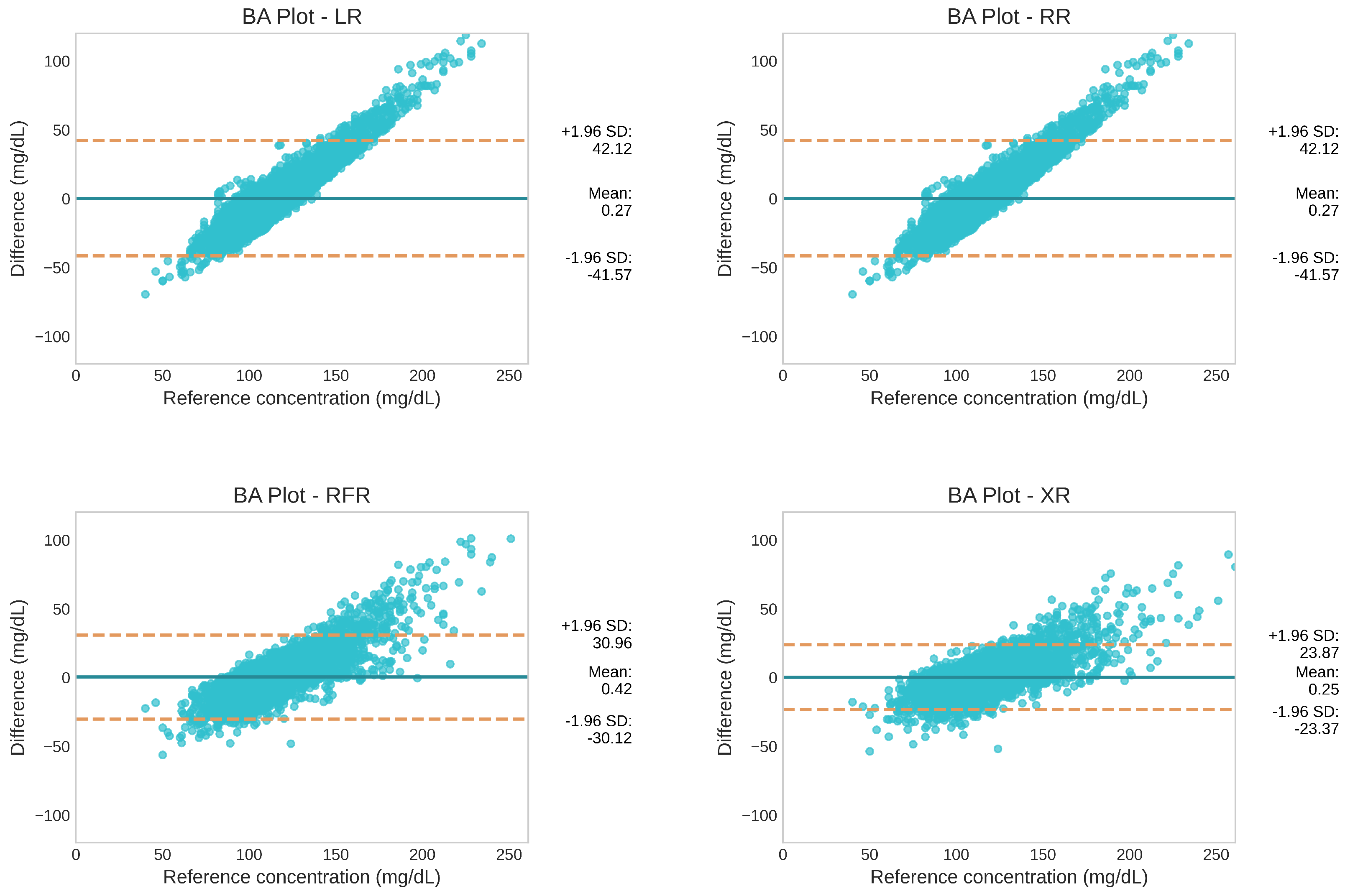
3.1.2. Level of Agreement
3.2. Clinical Accuracy
3.3. SHAP Explanations
4. Discussion
4.1. Feature Importance
4.2. Model Performance
4.3. Comparison with Prior Work
4.4. Clinical Applicability
4.5. Limitations
4.6. Future Work
5. Conclusions
Author Contributions
Funding
Institutional Review Board Statement
Informed Consent Statement
Data Availability Statement
Conflicts of Interest
References
- Faro, J.M.; Yue, K.L.; Singh, A.; Soni, A.; Ding, E.Y.; Shi, Q.; McManus, D.D. Wearable device use and technology preferences in cancer survivors with or at risk for atrial fibrillation. Cardiovasc. Digit. Health J. 2022, 3, S23–S27. [Google Scholar] [CrossRef]
- Gray, R.; Indraratna, P.; Lovell, N.; Ooi, S.Y. Digital health technology in the prevention of heart failure and coronary artery disease. Cardiovasc. Digit. Health J. 2022, 3, S9–S16. [Google Scholar] [CrossRef] [PubMed]
- Chong, K.P.L.; Guo, J.Z.; Deng, X.; Woo, B.K.P. Consumer Perceptions of Wearable Technology Devices: Retrospective Review and Analysis. JMIR mHealth uHealth 2020, 8, e17544. [Google Scholar] [CrossRef]
- Ringeval, M.; Wagner, G.; Denford, J.; Paré, G.; Kitsiou, S. Fitbit-Based Interventions for Healthy Lifestyle Outcomes: Systematic Review and Meta-Analysis. J. Med. Internet Res. 2020, 22, e23954. [Google Scholar] [CrossRef]
- Leucker, T.M.; Blaha, M.J.; Jones, S.R.; Vavuranakis, M.A.; Williams, M.S.; Lai, H.; Schindler, T.H.; Latina, J.; Schulman, S.P.; Gerstenblith, G. Effect of Evolocumab on Atherogenic Lipoproteins During the Peri- and Early Postinfarction Period. Circulation 2020, 142, 419–421. [Google Scholar] [CrossRef] [PubMed]
- Hosseinalizadeh, M.; Asghari, M.; Toosizadeh, N. Sensor-Based Frailty Assessment Using Fitbit. Sensors 2024, 24, 7827. [Google Scholar] [CrossRef]
- Hoang, N.H.; Liang, Z. Detection and Severity Classification of Sleep Apnea Using Continuous Wearable SpO2 Signals: A Multi-Scale Feature Approach. Sensors 2025, 25, 1698. [Google Scholar] [CrossRef]
- Zilu, L. Developing probabilistic ensemble machine learning models for home-based sleep apnea screening using overnight SpO2 data at varying data granularity. Sleep Breath. 2024, 28, 2409–2420. [Google Scholar]
- Pepplinkhuizen, S.; Hoeksema, W.F.; van der Stuijt, W.; van Steijn, N.J.; Winter, M.M.; Wilde, A.A.; Smeding, L.; Knops, R.E. Accuracy and clinical relevance of the single-lead Apple Watch electrocardiogram to identify atrial fibrillation. Cardiovasc. Digit. Health J. 2022, 3, S17–S22. [Google Scholar] [CrossRef]
- Mattison, G.; Canfell, O.J.; Forrester, D.; Dobbins, C.; Smith, D.; Reid, D.; Sullivan, C. A step in the right direction: The potential role of smartwatches in supporting chronic disease prevention in health care. Med. J. Aust. 2023, 218, 384–388. [Google Scholar] [CrossRef]
- Diabetes Facts and Figures|International Diabetes Federation. Available online: https://idf.org/about-diabetes/diabetes-facts-figures/ (accessed on 21 April 2025).
- Rooney, M.R.; Fang, M.; Ogurtsova, K.; Ozkan, B.; Echouffo-Tcheugui, J.B.; Boyko, E.J.; Magliano, D.J.; Selvin, E. Global Prevalence of Prediabetes. Diabetes Care 2023, 46, 1388–1394. [Google Scholar] [CrossRef]
- National Diabetes Statistics Report|Diabetes|CDC. Available online: https://www.cdc.gov/diabetes/php/data-research/?CDC_AAref_Val=https://www.cdc.gov/diabetes/pdfs/data/statistics/national-diabetes-statistics-report.pdf (accessed on 7 April 2025).
- Tabák, A.G.; Herder, C.; Rathmann, W.; Brunner, E.J.; Kivimäki, M. Prediabetes: A high-risk state for developing diabetes. Lancet 2012, 379, 2279. [Google Scholar] [CrossRef]
- Ehrhardt, N.; Zaghal, E.A. Continuous Glucose Monitoring As a Behavior Modification Tool. Clin. Diabetes A Publ. Am. Diabetes Assoc. 2020, 38, 126. [Google Scholar] [CrossRef] [PubMed]
- Layne, J.E.; Jepson, L.H.; Carite, A.M.; Parkin, C.G.; Bergenstal, R.M. Long-term improvements in glycemic control with Dexcom CGM use in adults with noninsulin-treated type 2 diabetes. Diabetes Technol. Ther. 2024, 26, 925–931. [Google Scholar] [CrossRef] [PubMed]
- Liang, Z. Exploring the Impact of Wearable Continuous Glucose Monitoring on Glucose Regulation and Eating Behavior in Healthy Individuals: A Pilot Study. In Proceedings of the Behavior Transformation by IoT International Workshop, Tokyo, Japan, 3–7 June 2024; Association for Computing Machinery: New York, NY, USA, 2024; pp. 7–12. [Google Scholar]
- Zhang, Y.; Pan, X.F.; Chen, J.; Xia, L.; Cao, A.; Zhang, Y.; Wang, J.; Li, H.; Yang, K.; Guo, K.; et al. Combined lifestyle factors and risk of incident type 2 diabetes and prognosis among individuals with type 2 diabetes: A systematic review and meta-analysis of prospective cohort studies. Diabetologia 2020, 63, 21–33. [Google Scholar] [CrossRef] [PubMed]
- Group, T.D.P.P.D.R. The Diabetes Prevention Program (DPP)Description of lifestyle intervention. Diabetes Care 2002, 25, 2165–2171. [Google Scholar]
- Mansour, M.; Darweesh, M.S.; Soltan, A. Wearable devices for glucose monitoring: A review of state-of-the-art technologies and emerging trends. Alex. Eng. J. 2024, 89, 224–243. [Google Scholar] [CrossRef]
- Klonoff, D.C.; Nguyen, K.T.; Xu, N.Y.; Gutierrez, A.; Espinoza, J.C.; Vidmar, A.P. Use of continuous glucose monitors by people without diabetes: An idea whose time has come? J. Diabetes Sci. Technol. 2023, 17, 1686–1697. [Google Scholar] [CrossRef]
- Malik, B.H.; Coté, G.L. Real-time, closed-loop dual-wavelength optical polarimetry for glucose monitoring. J. Biomed. Opt. 2010, 15, 017002. [Google Scholar] [CrossRef]
- Lan, Y.; Kuang, Y.; Zhou, L.; Wu, G.; Gu, P.; Wei, H.; Chen, K. Noninvasive monitoring of blood glucose concentration in diabetic patients with optical coherence tomography. Laser Phys. Lett. 2017, 14, 035603. [Google Scholar] [CrossRef]
- Buchert, J.M. Thermal emission spectroscopy as a tool for noninvasive blood glucose measurements. In Proceedings of the Optical Security and Safety, Warsaw, Poland, 2–4 August 2004; SPIE: St Bellingham, WA, USA, 2004; Volume 5566, pp. 100–111. [Google Scholar]
- Tura, A.; Sbrignadello, S.; Cianciavicchia, D.; Pacini, G.; Ravazzani, P. A low frequency electromagnetic sensor for indirect measurement of glucose concentration: In vitro experiments in different conductive solutions. Sensors 2010, 10, 5346–5358. [Google Scholar] [CrossRef] [PubMed]
- Gonzales, W.V.; Mobashsher, A.T.; Abbosh, A. The Progress of Glucose Monitoring—A Review of Invasive to Minimally and Non-Invasive Techniques, Devices and Sensors. Sensors 2019, 19, 800. [Google Scholar] [CrossRef] [PubMed]
- Russell, W.R.; Baka, A.; Björck, I.; Delzenne, N.; Gao, D.; Griffiths, H.R.; Hadjilucas, E.; Juvonen, K.; Lahtinen, S.; Lansink, M.; et al. Impact of Diet Composition on Blood Glucose Regulation. Crit. Rev. Food Sci. Nutr. 2016, 56, 541–590. [Google Scholar] [CrossRef] [PubMed]
- Amanat, S.; Ghahri, S.; Dianatinasab, A.; Fararouei, M.; Dianatinasab, M. Exercise and Type 2 Diabetes. Adv. Exp. Med. Biol. 2020, 1228, 91–105. [Google Scholar]
- Sharma, K.; Akre, S.; Chakole, S.; Wanjari, M.B. Stress-Induced Diabetes: A Review. Cureus 2022, 14, e29142. [Google Scholar] [CrossRef]
- Qian, J.; Scheer, F.A. Circadian System and Glucose Metabolism: Implications for Physiology and Disease. Trends Endocrinol. Metab. 2016, 27, 282–293. [Google Scholar] [CrossRef]
- Mauvais-Jarvis, F. Gender differences in glucose homeostasis and diabetes. Physiol. Behav. 2018, 187, 20–23. [Google Scholar] [CrossRef]
- Singh, J.P.; Larson, M.G.; O’Donnell, C.J.; Wilson, P.F.; Tsuji, H.; Lloyd-Jones, D.M.; Levy, D. Association of hyperglycemia with reduced heart rate variability (The Framingham Heart Study). Am. J. Cardiol. 2000, 86, 309–312. [Google Scholar] [CrossRef]
- Kenny, G.P.; Sigal, R.J.; McGinn, R. Body temperature regulation in diabetes. Temperature 2016, 3, 119–145. [Google Scholar] [CrossRef]
- Cordeiro, R.; Karimian, N.; Park, Y. Hyperglycemia Identification Using ECG in Deep Learning Era. Sensors 2021, 21, 6263. [Google Scholar] [CrossRef]
- Lehmann, V.; Foll, S.; Maritsch, M.; van Weenen, E.; Kraus, M.; Lagger, S.; Odermatt, K.; Albrecht, C.; Fleisch, E.; Zueger, T.; et al. Noninvasive Hypoglycemia Detection in People with Diabetes Using Smartwatch Data. Diabetes Care 2023, 46, 993–997. [Google Scholar] [CrossRef]
- van den Brink, W.J.; van den Broek, T.J.; Palmisano, S.; Wopereis, S.; de Hoogh, I.M. Digital Biomarkers for Personalized Nutrition: Predicting Meal Moments and Interstitial Glucose with Non-Invasive, Wearable Technologies. Nutrients 2022, 14, 4465. [Google Scholar] [CrossRef] [PubMed]
- Ali, H.; Niazi, I.K.; White, D.; Akhter, M.N.; Madanian, S. Comparison of Machine Learning Models for Predicting Interstitial Glucose Using Smart Watch and Food Log. Electronics 2024, 13, 3192. [Google Scholar] [CrossRef]
- Bent, B.; Cho, P.J.; Henriquez, M.; Wittmann, A.; Thacker, C.; Feinglos, M.; Crowley, M.J.; Dunn, J.P. Engineering digital biomarkers of interstitial glucose from noninvasive smartwatches. Npj Digit. Med. 2021, 4, 89. [Google Scholar] [CrossRef]
- Huang, X.; Schmelter, F.; Uhlig, A.; Irshad, M.T.; Nisar, M.A.; Piet, A.; Jablonski, L.; Witt, O.; Schröder, T.; Sina, C.; et al. Comparison of feature learning methods for non-invasive interstitial glucose prediction using wearable sensors in healthy cohorts: A pilot study. Intell. Med. 2024, 4, 226–238. [Google Scholar] [CrossRef]
- Bogue-Jimenez, B.; Huang, X.; Powell, D.; Doblas, A. Selection of Noninvasive Features in Wrist-Based Wearable Sensors to Predict Blood Glucose Concentrations Using Machine Learning Algorithms. Sensors 2022, 22, 3534. [Google Scholar] [CrossRef]
- Cho, P.; Kim, J.; Bent, B.; Dunn, J. BIG IDEAs Lab Glycemic Variability and Wearable Device Data. Version 1.1.2. PhysioNet 2023. Available online: https://physionet.org/content/big-ideas-glycemic-wearable/1.1.2/ (accessed on 21 April 2025).
- Goldberger, A.L.; Amaral, L.A.; Glass, L.; Hausdorff, J.M.; Ivanov, P.C.; Mark, R.G.; Mietus, J.E.; Moody, G.B.; Peng, C.K.; Stanley, H.E. PhysioBank, PhysioToolkit, and PhysioNet: Components of a new research resource for complex physiologic signals. Circulation 2000, 101, E215–E220. [Google Scholar] [CrossRef] [PubMed]
- van Gent, P.; Farah, H.; van Nes, N.; van Arem, B. HeartPy: A novel heart rate algorithm for the analysis of noisy signals. Transp. Res. Part F Traffic Psychol. Behav. 2019, 66, 368–378. [Google Scholar] [CrossRef]
- Fridolfsson, J.; Börjesson, M.; Buck, C.; Ekblom, Ö.; Ekblom-Bak, E.; Hunsberger, M.; Lissner, L.; Arvidsson, D. Effects of Frequency Filtering on Intensity and Noise in Accelerometer-Based Physical Activity Measurements. Sensors 2019, 19, 2186. [Google Scholar] [CrossRef]
- Posada-Quintero, H.F.; Chon, K.H. Innovations in Electrodermal Activity Data Collection and Signal Processing: A Systematic Review. Sensors 2020, 20, 479. [Google Scholar] [CrossRef]
- Föll, S.; Maritsch, M.; Spinola, F.; Mishra, V.; Barata, F.; Kowatsch, T.; Fleisch, E.; Wortmann, F. FLIRT: A feature generation toolkit for wearable data. Comput. Methods Prog. Biomed. 2021, 212, 106461. [Google Scholar] [CrossRef] [PubMed]
- Liang, Z. Novel method combining multiscale attention entropy of overnight blood oxygen level and machine learning for easy sleep apnea screening. Digital Health 2023, 9, 20552076231211550. [Google Scholar] [CrossRef] [PubMed]
- Flood, M.W.; Grimm, B. EntropyHub: An open-source toolkit for entropic time series analysis. PLoS ONE 2021, 16, e0259448. [Google Scholar] [CrossRef]
- Pessa, A.A.; Ribeiro, H.V. Ordpy: A Python package for data analysis with permutation entropy and ordinal network methods. Chaos 2021, 31, 063110. [Google Scholar] [CrossRef] [PubMed]
- Rawald, T.; Sips, M.; Marwan, N. PyRQA—Conducting recurrence quantification analysis on very long time series efficiently. Comput. Geosci. 2017, 104, 101–108. [Google Scholar] [CrossRef]
- Multi-Modal Feature Engineering for Non-Invasive Glucose Prediction. Available online: https://www.researchgate.net/publication/391803833_Multi-modal_Feature_Engineering_for_Non-invasive_Glucose_Prediction (accessed on 16 May 2025).
- Berisha, V.; Krantsevich, C.; Hahn, P.R.; Hahn, S.; Dasarathy, G.; Turaga, P.; Liss, J. Digital medicine and the curse of dimensionality. Npj Digit. Med. 2021, 4, 153. [Google Scholar] [CrossRef]
- Altman, N.; Krzywinski, M. The curse(s) of dimensionality. Nat. Methods 2018, 15, 399–400. [Google Scholar] [CrossRef]
- Kapoor, S.; Narayanan, A. Leakage and the reproducibility crisis in machine-learning-based science. Patterns 2023, 4, 100804. [Google Scholar] [CrossRef]
- Krouwer, J.S. Why Bland-Altman plots should use X, not (Y + X)/2 when X is a reference method. Stat. Med. 2008, 27, 778–780. [Google Scholar] [CrossRef]
- Altman, D.G.; Bland, J.M. Measurement in Medicine: The Analysis of Method Comparison Studies. Statistician 1983, 32, 307. [Google Scholar] [CrossRef]
- Clarke, W.L.; Cox, D.; Gonder-Frederick, L.A.; Carter, W.; Pohl, S.L. Evaluating Clinical Accuracy of Systems for Self-Monitoring of Blood Glucose. Diabetes Care 1987, 10, 622–628. [Google Scholar] [CrossRef] [PubMed]
- Lundberg, S.M.; Lee, S.I. A unified approach to interpreting model predictions. In Proceedings of the 31st International Conference on Neural Information Processing Systems, Long Beach, CA, USA, 4–9 December 2017; pp. 4766–4775. [Google Scholar]
- Freckmann, G.; Pleus, S.; Grady, M.; Setford, S.; Levy, B. Measures of Accuracy for Continuous Glucose Monitoring and Blood Glucose Monitoring Devices. J. Diabetes Sci. Technol. 2019, 13, 575–583. [Google Scholar] [CrossRef] [PubMed]
- Siegmund, T.; Heinemann, L.; Kolassa, R.; Thomas, A. Discrepancies between blood glucose and interstitial glucose—technological artifacts or physiology: Implications for selection of the appropriate therapeutic target. J. Diabetes Sci. Technol. 2017, 11, 766–772. [Google Scholar] [CrossRef] [PubMed]


| Item | Categories | Value |
|---|---|---|
| Number of subjects | 16 | |
| Age range | 35–65 years | |
| Gender | Male | 7 (43.75%) |
| Female | 9 (56.25%) | |
| HbA1c | 5.7 ± 0.3 | |
| Glucose Metrics 1 | Average glucose | 115 mg/dL |
| Time in range (TIR) 2 | 97.87% | |
| Time above range (TAR) 3 | 1.57% | |
| Time below range (TBR) 4 | 0.56% | |
| No. of epochs 1 | 26,380 |
| Model Name | R-Squared | RMSE (mg/dL) | NRMSE (mg/dL) | MARD (%) |
|---|---|---|---|---|
| LR | 0.13 ± 0.01 | 21.3 ± 0.3 | 0.93 ± 0.00 | 13.7 ± 0.1 |
| RR | 0.13 ± 0.01 | 21.3 ± 0.3 | 0.93 ± 0.00 | 13.7 ± 0.1 |
| RFR | 0.53 ± 0.01 | 15.6 ± 0.3 | 0.68 ± 0.01 | 9.7 ± 0.1 |
| XR | 0.73 ± 0.01 | 11.9 ± 0.3 | 0.52 ± 0.01 | 7.1 ± 0.1 |
| Model Name | Zone A (%) | Zone B (%) | Zone C (%) | Zone D (%) | Zone E (%) | Zones (A + B) (%) |
|---|---|---|---|---|---|---|
| LR | 77.0 | 22.2 | 0.0 | 0.8 | 0.0 | 99.2 |
| RR | 77.0 | 22.2 | 0.0 | 0.8 | 0.0 | 99.2 |
| RFR | 89.1 | 10.3 | 0.0 | 0.6 | 0.0 | 99.4 |
| XR | 94.2 | 5.2 | 0.0 | 0.6 | 0.0 | 99.4 |
Disclaimer/Publisher’s Note: The statements, opinions and data contained in all publications are solely those of the individual author(s) and contributor(s) and not of MDPI and/or the editor(s). MDPI and/or the editor(s) disclaim responsibility for any injury to people or property resulting from any ideas, methods, instructions or products referred to in the content. |
© 2025 by the authors. Licensee MDPI, Basel, Switzerland. This article is an open access article distributed under the terms and conditions of the Creative Commons Attribution (CC BY) license (https://creativecommons.org/licenses/by/4.0/).
Share and Cite
Karunarathna, T.S.; Liang, Z. Development of Non-Invasive Continuous Glucose Prediction Models Using Multi-Modal Wearable Sensors in Free-Living Conditions. Sensors 2025, 25, 3207. https://doi.org/10.3390/s25103207
Karunarathna TS, Liang Z. Development of Non-Invasive Continuous Glucose Prediction Models Using Multi-Modal Wearable Sensors in Free-Living Conditions. Sensors. 2025; 25(10):3207. https://doi.org/10.3390/s25103207
Chicago/Turabian StyleKarunarathna, Thilini S., and Zilu Liang. 2025. "Development of Non-Invasive Continuous Glucose Prediction Models Using Multi-Modal Wearable Sensors in Free-Living Conditions" Sensors 25, no. 10: 3207. https://doi.org/10.3390/s25103207
APA StyleKarunarathna, T. S., & Liang, Z. (2025). Development of Non-Invasive Continuous Glucose Prediction Models Using Multi-Modal Wearable Sensors in Free-Living Conditions. Sensors, 25(10), 3207. https://doi.org/10.3390/s25103207