

Multi-Feature Fusion Method Based on Adaptive Dilation Convolution for Small-Object Detection

Abstract
1. Introduction
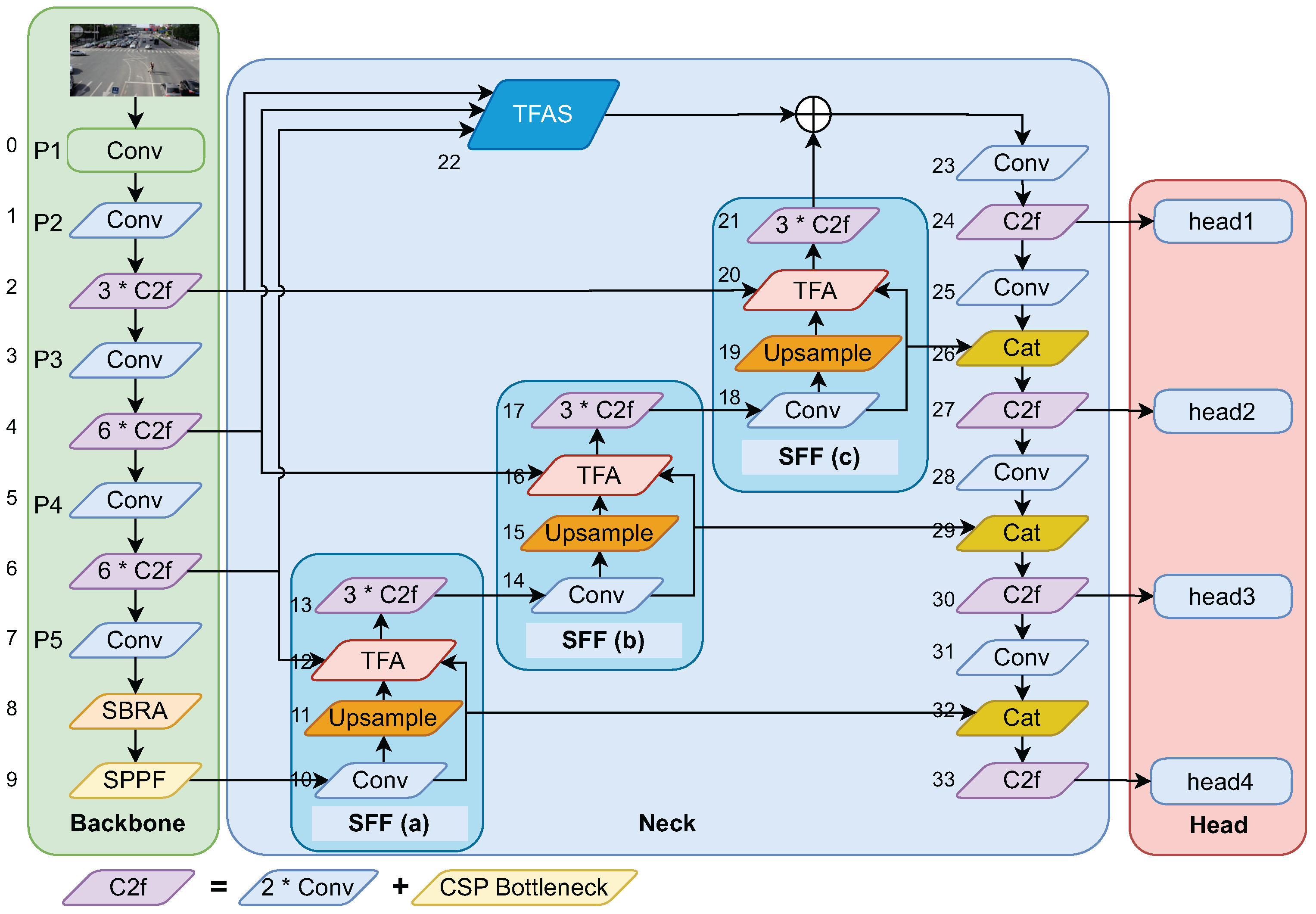
- Based on the YOLOv8 object detection architecture, a new feature fusion architecture is proposed, which consists of three multi-scale feature fusion modules, a triple-feature encoding module, and a downsampling process, that can fuse the features of different scales from the backbone network. The proposed architecture is used to verify the accuracy of radar detection, laying the foundation for the post-fusion technology of radar and cameras.
- A new triple-feature coding module is proposed, which performs different processing on the features of three different scales. Adaptive dilated convolution is applied to features of different frequency bands (corresponding to object scales) with varying dilation rates, reducing intra-class size variance in feature maps and enabling dynamic receptive field adaptation.
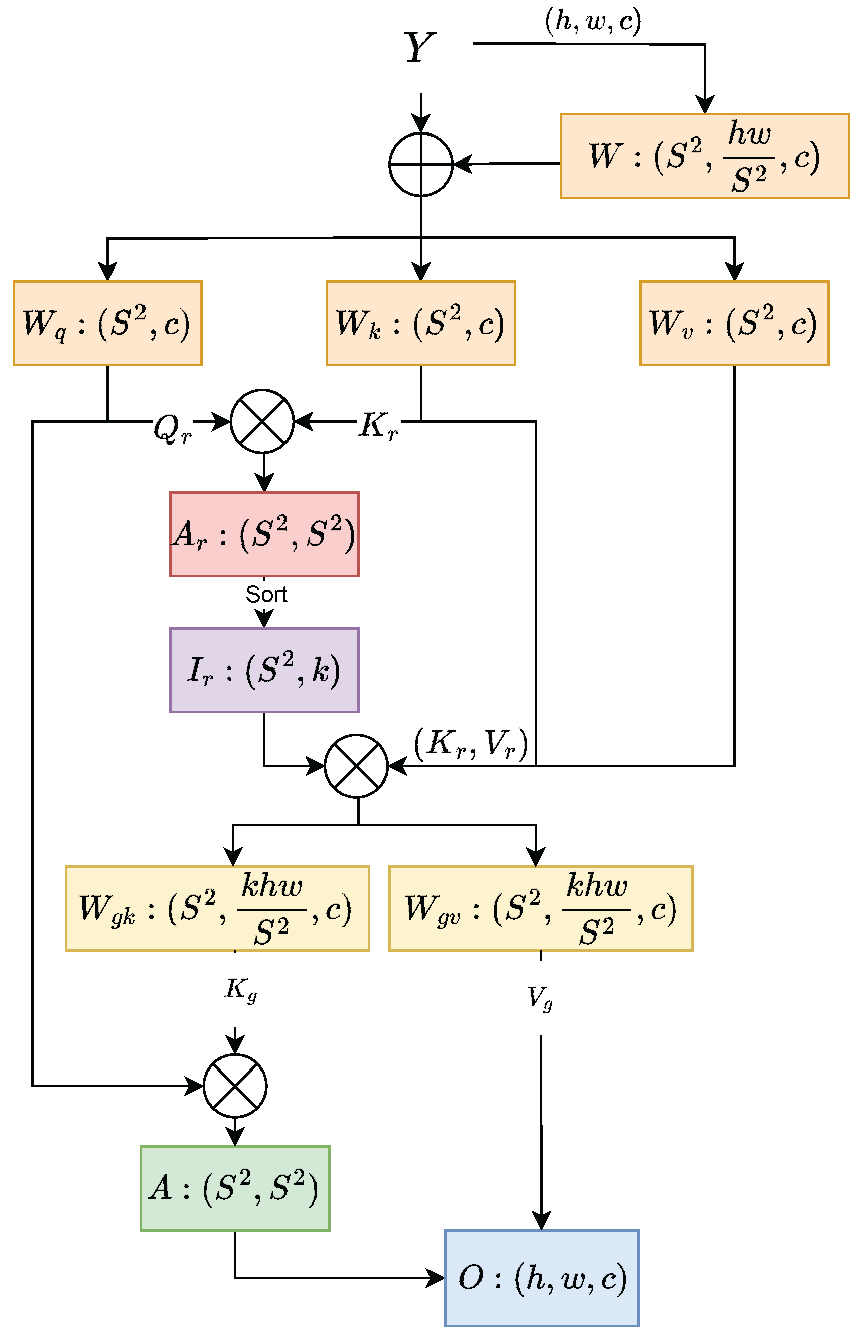
- A new self-attention module is proposed and added to the original CSPDarknet backbone network, which captures global dependencies through a token-to-token self-attention mechanism to bring about better context analysis, resulting in the learning of more distinguishable feature representations.
2. Related Work
2.1. Small-Object Detection
2.2. Attention Mechanism
2.3. Feature Fusion
2.4. Radar and Camera System
3. Methodology
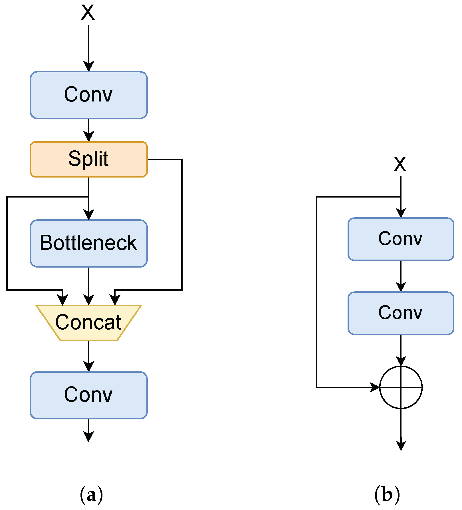
3.1. Backbone
3.2. Neck
3.3. Head
4. Experiments
4.1. Datasets
4.2. Evaluation Protocols and Implementation Details
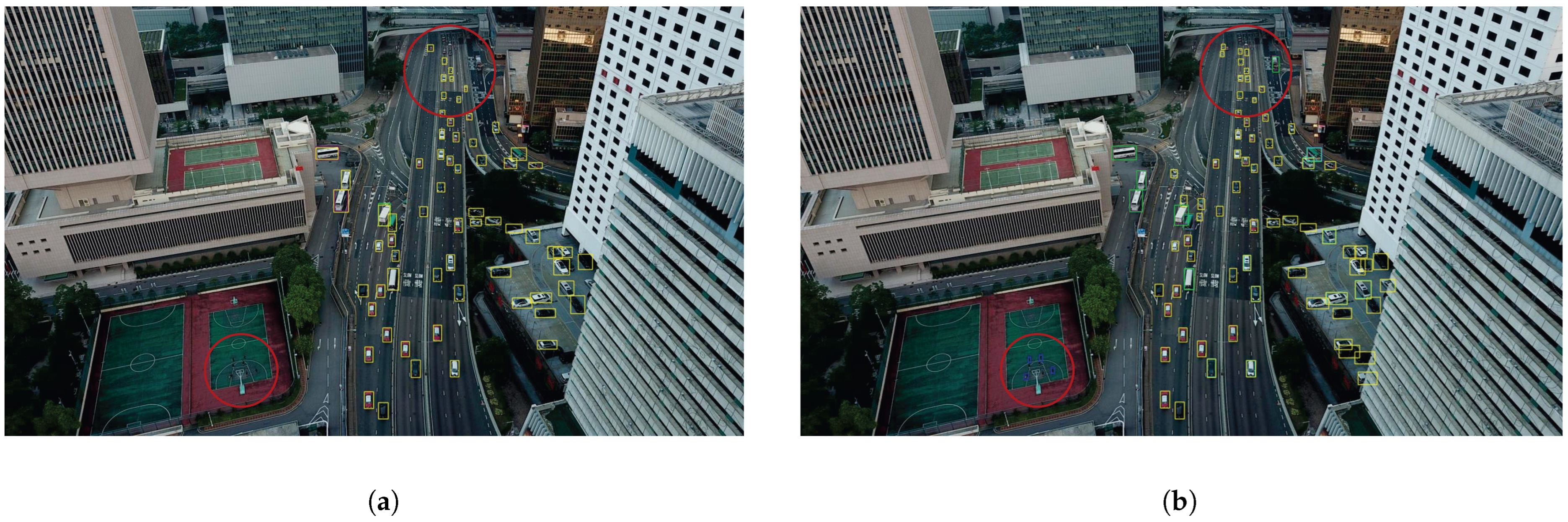
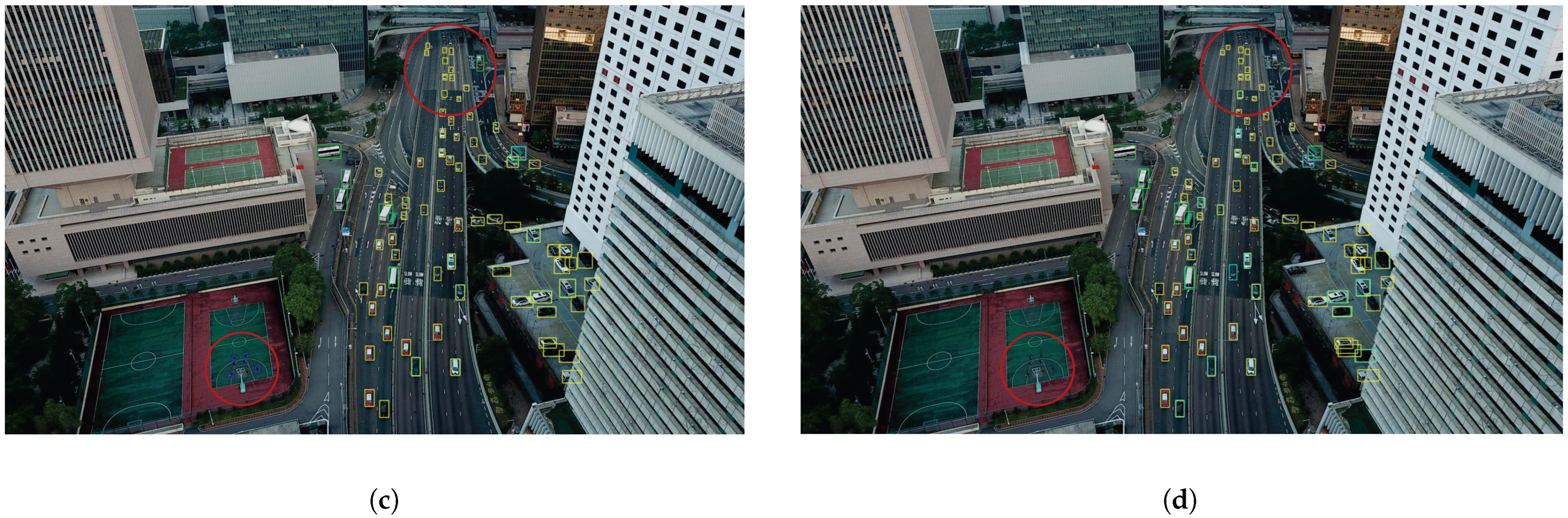
4.3. Object Detection in VisDrone2019
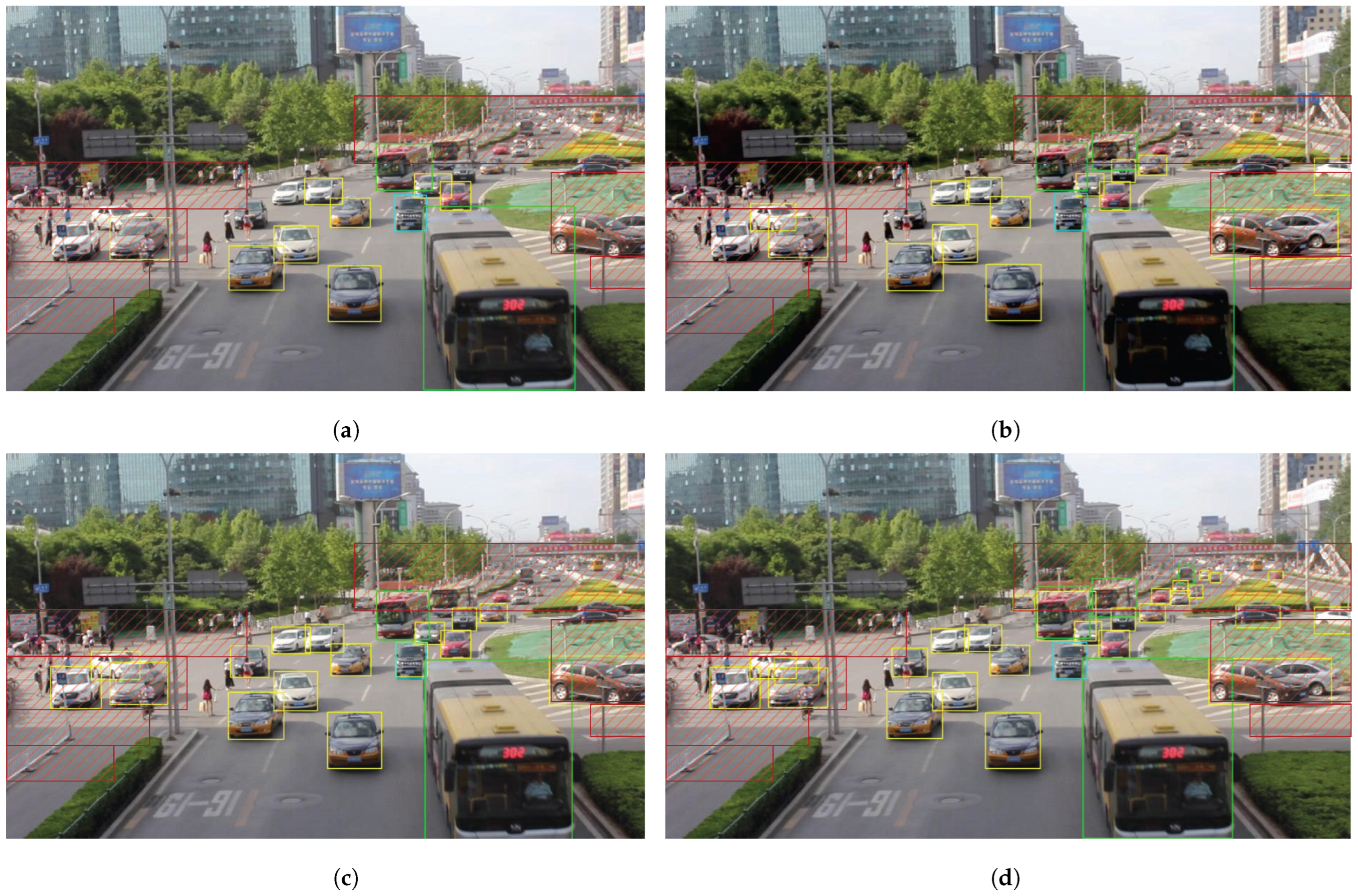
4.4. Object Detection in UA-DETRAC
4.5. Ablation Studies and Complexity Studies
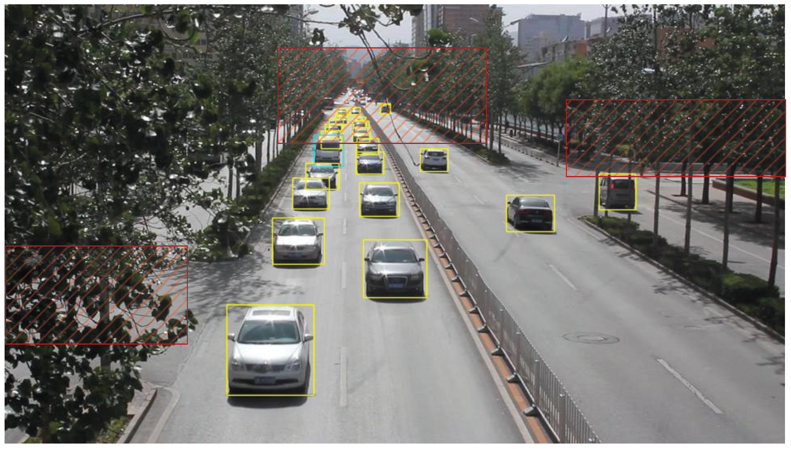
4.6. Physical Experiment
5. Conclusions
Author Contributions
Funding
Institutional Review Board Statement
Informed Consent Statement
Data Availability Statement
Conflicts of Interest
References
- Zhou, X.; Shen, K.; Liu, Z. ADMNet: Attention-guided densely multi-scale network for lightweight salient object detection. IEEE Trans. Multimed. 2024, 26, 10828–10841. [Google Scholar] [CrossRef]
- Xu, S.; Chen, Z.; Zhang, H.; Xue, L.; Su, H. Improved remote sensing image target detection based on YOLOv7. Optoelectron. Lett. 2024, 20, 234–242. [Google Scholar] [CrossRef]
- Ren, S.; He, K.; Girshick, R.; Sun, J. Faster R-CNN: Towards real-time object detection with region proposal networks. IEEE Trans. Pattern Anal. Mach. Intell. 2016, 39, 1137–1149. [Google Scholar] [CrossRef] [PubMed]
- Deng, J.; Dong, W.; Socher, R.; Li, L.J.; Li, K.; Li, F.-F. Imagenet: A large-scale hierarchical image database. In Proceedings of the 2009 IEEE Conference on Computer Vision and Pattern Recognition, Miami, FL, USA, 20–25 June 2009; pp. 248–255. [Google Scholar]
- Liu, W.; Anguelov, D.; Erhan, D.; Szegedy, C.; Reed, S.; Fu, C.Y.; Berg, A.C. Ssd: Single shot multibox detector. In Proceedings of the Computer Vision–ECCV 2016: 14th European Conference, Amsterdam, The Netherlands, 11–14 October 2016; Proceedings, Part I 14. Springer: Berlin/Heidelberg, Germany, 2016; pp. 21–37. [Google Scholar]
- Qin, H.; Wang, J.; Mao, X.; Zhao, Z.; Gao, X.; Lu, W. An improved faster R-CNN method for landslide detection in remote sensing images. J. Geovis. Spat. Anal. 2024, 8, 2. [Google Scholar] [CrossRef]
- Redmon, J. You only look once: Unified, real-time object detection. In Proceedings of the IEEE Conference on Computer Vision and Pattern Recognition, Las Vegas, NV, USA, 27–30 June 2016. [Google Scholar]
- He, K.; Gkioxari, G.; Dollár, P.; Girshick, R. Mask r-cnn. In Proceedings of the IEEE international Conference on Computer Vision, Venice, Italy, 22–29 October 2017; pp. 2961–2969. [Google Scholar]
- Carion, N.; Massa, F.; Synnaeve, G.; Usunier, N.; Kirillov, A.; Zagoruyko, S. End-to-end object detection with transformers. In Proceedings of the European Conference on Computer Vision, Glasgow, UK, 23–28 August 2020; Springer: Berlin/Heidelberg, Germany, 2020; pp. 213–229. [Google Scholar]
- Li, Y.; Chen, Y.; Wang, N.; Zhang, Z. Scale-aware trident networks for object detection. In Proceedings of the IEEE/CVF International Conference on Computer Vision, Seoul, Republic of Korea, 27 October–2 November 2019; pp. 6054–6063. [Google Scholar]
- Bai, Y.; Zhang, Y.; Ding, M.; Ghanem, B. Sod-mtgan: Small object detection via multi-task generative adversarial network. In Proceedings of the European Conference on Computer Vision (ECCV), Munich, Germany, 8–14 September 2018; pp. 206–221. [Google Scholar]
- Zhu, L.; Wang, X.; Ke, Z.; Zhang, W.; Lau, R.W. Biformer: Vision transformer with bi-level routing attention. In Proceedings of the IEEE/CVF Conference on Computer Vision and Pattern Recognition, Vancouver, BC, Canada, 18–22 June 2023; pp. 10323–10333. [Google Scholar]
- Kisantal, M. Augmentation for Small Object Detection. arXiv 2019, arXiv:1902.07296. [Google Scholar]
- Cheng, G.; Yuan, X.; Yao, X.; Yan, K.; Zeng, Q.; Xie, X.; Han, J. Towards large-scale small object detection: Survey and benchmarks. IEEE Trans. Pattern Anal. Mach. Intell. 2023, 45, 13467–13488. [Google Scholar] [CrossRef] [PubMed]
- Meethal, A.; Granger, E.; Pedersoli, M. Cascaded zoom-in detector for high resolution aerial images. In Proceedings of the IEEE/CVF Conference on Computer Vision and Pattern Recognition, Vancouver, BC, Canada, 18–22 June 2023; pp. 2046–2055. [Google Scholar]
- Zhou, X.; Wang, D.; Krähenbühl, P. Objects as points. arXiv 2019, arXiv:1904.07850. [Google Scholar]
- Fujitake, M.; Sugimoto, A. Video sparse transformer with attention-guided memory for video object detection. IEEE Access 2022, 10, 65886–65900. [Google Scholar] [CrossRef]
- Huang, S.; Lu, Z.; Cun, X.; Yu, Y.; Zhou, X.; Shen, X. DEIM: DETR with Improved Matching for Fast Convergence. arXiv 2024, arXiv:2412.04234. [Google Scholar]
- Perreault, H.; Bilodeau, G.A.; Saunier, N.; Héritier, M. Spotnet: Self-attention multi-task network for object detection. In Proceedings of the 2020 17th Conference on Computer and Robot Vision (CRV), Ottawa, ON, Canada, 13–15 May 2020; pp. 230–237. [Google Scholar]
- Zhu, X.; Lyu, S.; Wang, X.; Zhao, Q. TPH-YOLOv5: Improved YOLOv5 based on transformer prediction head for object detection on drone-captured scenarios. In Proceedings of the IEEE/CVF International Conference on Computer Vision, Montreal, BC, Canada, 11–17 October 2021; pp. 2778–2788. [Google Scholar]
- Perreault, H.; Bilodeau, G.A.; Saunier, N.; Héritier, M. FFAVOD: Feature fusion architecture for video object detection. Pattern Recognit. Lett. 2021, 151, 294–301. [Google Scholar] [CrossRef]
- Liu, S.; Qi, L.; Qin, H.; Shi, J.; Jia, J. Path aggregation network for instance segmentation. In Proceedings of the IEEE Conference on Computer Vision and Pattern Recognition, Salt Lake City, UT, USA, 18–22 June 2018; pp. 8759–8768. [Google Scholar]
- Chen, L.; Gu, L.; Zheng, D.; Fu, Y. Frequency-Adaptive Dilated Convolution for Semantic Segmentation. In Proceedings of the IEEE/CVF Conference on Computer Vision and Pattern Recognition, Seattle, WA, USA, 17–18 June 2024; pp. 3414–3425. [Google Scholar]
- Yang, B.; Zhang, H. A CFAR algorithm based on Monte Carlo method for millimeter-wave radar road traffic target detection. Remote Sens. 2022, 14, 1779. [Google Scholar] [CrossRef]
- Xu, D.; Liu, Y.; Wang, Q.; Wang, L.; Liu, R. Target detection based on improved Hausdorff distance matching algorithm for millimeter-wave radar and video fusion. Sensors 2022, 22, 4562. [Google Scholar] [CrossRef] [PubMed]
- Qin, F.; Bu, X.; Liu, Y.; Liang, X.; Xin, J. Foreign object debris automatic target detection for millimeter-wave surveillance radar. Sensors 2021, 21, 3853. [Google Scholar] [CrossRef] [PubMed]
- Naseer, M.M.; Ranasinghe, K.; Khan, S.H.; Hayat, M.; Shahbaz Khan, F.; Yang, M.H. Intriguing properties of vision transformers. Adv. Neural Inf. Process. Syst. 2021, 34, 23296–23308. [Google Scholar]
- Lim, J.S.; Astrid, M.; Yoon, H.J.; Lee, S.I. Small object detection using context and attention. In Proceedings of the 2021 international Conference on Artificial intelligence in information and Communication (ICAIIC), Jeju Island, Republic of Korea, 20–23 April 2021; pp. 181–186. [Google Scholar]
- Wen, L.; Du, D.; Cai, Z.; Lei, Z.; Chang, M.C.; Qi, H.; Lim, J.; Yang, M.H.; Lyu, S. UA-DETRAC: A new benchmark and protocol for multi-object detection and tracking. Comput. Vis. Image Underst. 2020, 193, 102907. [Google Scholar] [CrossRef]
- Zhu, P.; Wen, L.; Bian, X.; Ling, H.; Hu, Q. Vision meets drones: A challenge. arXiv 2018, arXiv:1804.07437. [Google Scholar]


| Methods | mAP | AP50 | AP75 | APs | APm | APl |
|---|---|---|---|---|---|---|
| YOLOv8-x6 | 29.12 | 46.91 | 30.78 | 27.16 | 32.19 | 35.48 |
| DEIM | 29.50 | 49.54 | 30.99 | 20.31 | 41.95 | 55.10 |
| CZ Det. | 33.13 | 57.45 | 32.78 | 26.05 | 42.17 | 43.24 |
| TPH-YOLO | 35.74 | 57.31 | - | - | - | - |
| Ours | 38.88 | 59.12 | 37.25 | 28.37 | 43.38 | 44.52 |
| Methods | All | Pedestrian | People | Bicycle | Car | Van | Truck | Tricycle | Awning Tricycle | Bus | Motor |
|---|---|---|---|---|---|---|---|---|---|---|---|
| YOLOv8-x6 | 29.12 | 21.57 | 13.32 | 11.83 | 52.75 | 46.33 | 38.43 | 21.91 | 18.74 | 50.56 | 23.45 |
| DEIM | 32.45 | 22.47 | 12.03 | 11.97 | 57.34 | 46.52 | 41.33 | 22.42 | 18.94 | 56.43 | 25.47 |
| CZ Det. | 33.13 | 24.25 | 12.57 | 12.04 | 61.72 | 46.58 | 42.24 | 23.31 | 19.56 | 57.69 | 26.31 |
| TPH-YOLO | 37.21 | 28.87 | 16.76 | 15.54 | 68.93 | 50.19 | 45.09 | 27.32 | 23.67 | 63.27 | 30.58 |
| Ours | 38.88 | 29.93 | 18.44 | 16.32 | 69.81 | 49.76 | 46.32 | 27.87 | 24.21 | 61.78 | 31.45 |
| Methods | mAP | AP0.5 | AP0.75 |
|---|---|---|---|
| CenterNet | 83.52 | 96.46 | 91.23 |
| SpotNet | 86.78 | 96.72 | 91.38 |
| FFAVOD | 88.06 | 97.87 | 91.75 |
| VSTAM | 90.26 | 98.13 | 92.41 |
| Ours | 91.37 | 98.45 | 92.57 |
| Methods | mAP | AP50 | AP75 | APs | APm | APl | Params | FLOPs |
|---|---|---|---|---|---|---|---|---|
| baseline | 29.12 | 46.91 | 30.78 | 21.16 | 32.19 | 35.48 | 78M | 165B |
| +SBRA | 33.58 | 54.29 | 34.11 | 24.36 | 36.15 | 39.27 | 113M | 198B |
| +SBRA+TFA | 35.72 | 58.31 | 36.47 | 25.78 | 38.64 | 42.58 | 136M | 225B |
| +SBRA+TFA+TFAS | 38.88 | 59.12 | 37.25 | 28.37 | 43.38 | 44.52 | 168M | 247B |
| Distance (m) | AP | Car | Truck | Bus |
|---|---|---|---|---|
| 99.1 | 99.2 | 98.7 | 99.4 | |
| 81.5 | 81.3 | 80.8 | 82.3 | |
| 57.6 | 57.7 | 55.1 | 59.4 |
Disclaimer/Publisher’s Note: The statements, opinions and data contained in all publications are solely those of the individual author(s) and contributor(s) and not of MDPI and/or the editor(s). MDPI and/or the editor(s) disclaim responsibility for any injury to people or property resulting from any ideas, methods, instructions or products referred to in the content. |
© 2025 by the authors. Licensee MDPI, Basel, Switzerland. This article is an open access article distributed under the terms and conditions of the Creative Commons Attribution (CC BY) license (https://creativecommons.org/licenses/by/4.0/).
Share and Cite
Cao, L.; Wu, J.; Zhao, Z.; Fu, C.; Wang, D. Multi-Feature Fusion Method Based on Adaptive Dilation Convolution for Small-Object Detection. Sensors 2025, 25, 3182. https://doi.org/10.3390/s25103182
Cao L, Wu J, Zhao Z, Fu C, Wang D. Multi-Feature Fusion Method Based on Adaptive Dilation Convolution for Small-Object Detection. Sensors. 2025; 25(10):3182. https://doi.org/10.3390/s25103182
Chicago/Turabian StyleCao, Lin, Jin Wu, Zongmin Zhao, Chong Fu, and Dongfeng Wang. 2025. "Multi-Feature Fusion Method Based on Adaptive Dilation Convolution for Small-Object Detection" Sensors 25, no. 10: 3182. https://doi.org/10.3390/s25103182
APA StyleCao, L., Wu, J., Zhao, Z., Fu, C., & Wang, D. (2025). Multi-Feature Fusion Method Based on Adaptive Dilation Convolution for Small-Object Detection. Sensors, 25(10), 3182. https://doi.org/10.3390/s25103182