

Research on Collaborative Delivery Path Planning for Trucks and Drones in Parcel Delivery

Abstract
1. Introduction
- A multi-objective optimization model is developed to solve the TDCRPTW, considering both capacity constraints and time window restrictions in the multi-truck, multi-drone scenario.
- In the study of truck–drone collaborative delivery, the concept of time reliability is introduced by this paper for the first time, addressing the needs of both logistics companies and customers by minimizing time reliability and delivery costs.
- A two-stage strategy that integrates the self-adaptive k-means++ and temperature-controlled memory simulated annealing (TCMSA) approaches is proposed to solve the established model.
2. Materials and Methods
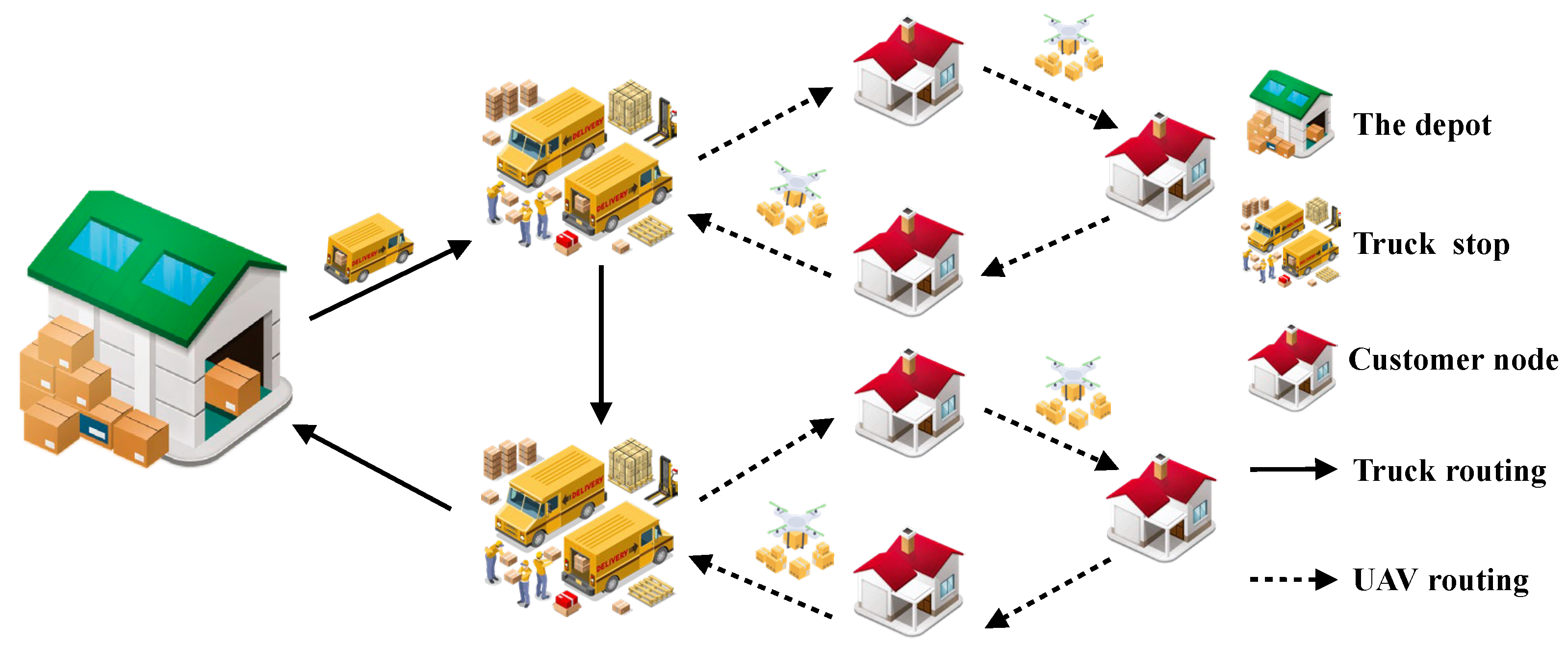
2.1. Problem Assumptions
- Within the maximum load and mileage of the trucks and drones, the impact of travel speed on the travel range of trucks and drones is not considered.
- The drone is considered to have completed a delivery upon arrival at the customer point, with unloading and receiving time not being considered at the customer node.
- While conducting drone deliveries to customer nodes, the truck remains stationary at a truck stop.
- Situations where delivery is hindered or delayed by causes beyond control are not taken into account.
- The depot holds commodities that have consistent requirements.
- Trucks and drones do not carry a load that exceeds their maximum load capacity.
2.2. Explanation of Parameters and Variables
2.3. Objective
2.3.1. Minimizing Total Economic Cost
2.3.2. Maximizing Time Reliability
2.4. Model Constraints
2.5. Optimization Algorithm
2.5.1. Truck Stop Location Strategy
| Algorithm 1 Pseudo-Code of Self-adaptive k-means++ Algorithm | |
| 1 | Input: Customer node, truck information, and parameters |
| 2 | Output: Coordinates and capacity of each cluster and the cluster centers (truck stopping points) %The output result is a cell array, where the first sublist of the cell array represents the truck docking points, and the remaining sublists correspond to the customer points contained within each truck docking point. |
| 3 | Initialize cluster centers randomly from data. %Adaptively set the value of k by searching for the best k within a certain range. |
| 4 | For each k in the given range of cluster numbers do |
| 5 | For each iteration in the range of Max number of iterations do |
| 6 | Compute distances from each data point to each cluster center. |
| 7 | For each data point do |
| 8 | Assign to the nearest cluster based on distance. %Ensure that each category satisfies the capacity constraint. |
| 9 | Check capacity constraint (14) and constraint (16) |
| 10 | If the assigned cluster exceeds capacity then |
| 11 | Find the next best cluster for the assignment. |
| 12 | End If |
| 13 | End For |
| 14 | Update cluster centers based on assigned points |
| 15 | Check for convergence based on the center change threshold. |
| 16 | Calculate the silhouette score for the current k and save |
| 17 | End For |
| 18 | End For |
| 19 | Determine the best k based on the maximum silhouette score. |
2.5.2. Truck–Drone Collaborative Routing Optimization
| Algorithm 2 Pseudo-Code of TCMSA Algorithm | |
| 1: | Input: Clustering results, truck and drone delivery costs, algorithm parameters |
| 2: | Output: Best route, best cost, time, and time reliability |
| 3: | For f in the cell array composed of truck docking points and clustering results do |
| %After solving the previous clustering algorithm, the first sublist in the cell array represents the truck docking points, while the remaining sublists correspond to the customer points within each truck docking point. Therefore, the truck route should be solved when f = 1 | |
| 4: | If f stays in the truck docking points array (f = 1) then |
| %To facilitate computer recognition, trucks and drones are labeled, where flag = 0 represents solving the truck route, and flag = 1 represents solving the drone route. | |
| 5: | Optimize the truck route and mark flag = 0 |
| 6: | Construct initial solution |
| 7: | Decode the initial solution and calculate the initial cost |
| %Outer loop | |
| 8: | For outIteriter in range of Max number of iterations do |
| %Inner loop | |
| 9: | For inIteriter in range of Max number of iterations do |
| %Ensure that the current solution satisfies the capacity constraint in the model. | |
| 10: | Generate neighborhood solutions under various constraints |
| 11: | Decode the new solution |
| 12: | Calculate the cost of the new solution |
| 13: | If the new solution’s objective compared to the current solution satisfies Pareto Best Solution then |
| 14: | Update the current solution |
| 15: | Else |
| %Calculate the probability of accepting the new solution | |
| 16: | calculate the probability M of accepting the new solution |
| 17: | If random number <= M then |
| 18: | accept the new solution, update the current solution |
| 19: | End If |
| 20: | End If |
| %If the new solution satisfies the requirements of the Pareto frontier, update the current solution. | |
| 21: | If the new solution’s objective compared to the Pareto frontier satisfies Pareto best Solution then |
| 22: | Update the current solution to the best Pareto frontier |
| 23: | Else |
| 24: | End If |
| 25: | End For |
| 26: | update temperature |
| 27: | record the best solution of each outer iteration |
| 28: | End For |
| 29: | Else |
| 30: | optimize the drone route and mark flag = 1 |
| 31: | follow the steps consistent with optimizing the truck route |
| 32: | End If |
| 33: | record the total global best solution for both truck and drone |
| 34: | End For |
| 35: | %The above describes the process for solving the truck route. The process for solving the drone route is the same as that for the truck route. |
- Setting Initial Parameters
- 2.
- Initial Feasible Solution
- 3.
- Generating New Solutions
- Swap Structure
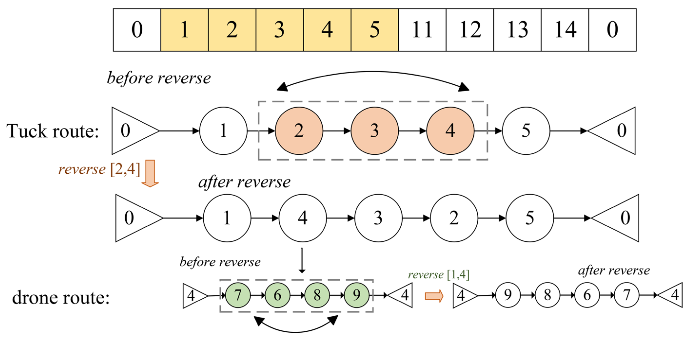
- Reverse Structure
- Insertion Structure
- 4.
- Updating the Best Solution:
- Improved Metropolis criterion
- Pareto frontier
- 5.
- Termination
3. Results
3.1. Experimental Setup and Parameter Settings
- Example Description
- 2.
- k-means++ Parameter Settings
- 3.
- TCMSA Parameter Settings
3.2. Model Performance Comparison
3.2.1. Large-Scale Case Results
3.2.2. Medium- and Small-Scale Case Results
3.3. Algorithm Performance Comparison
3.3.1. Clustering Performance
3.3.2. TCMSA Performance
4. Discussion
Author Contributions
Funding
Institutional Review Board Statement
Informed Consent Statement
Data Availability Statement
Conflicts of Interest
References
- Giones, F.; Brem, A. From toys to tools: The co-evolution of technological and entrepreneurial developments in the drone industry. Bus. Horiz. 2017, 60, 875–884. [Google Scholar] [CrossRef]
- Li, Y.; He, H.; Yang, D.; Fang, J. Geolocalization with aerial image sequence for UAVs. Auton. Robot. 2020, 44, 1199–1215. [Google Scholar] [CrossRef]
- Toscano, F.; Pierri, F.; Cutolo, A. Unmanned Aerial Vehicle for Precision Agriculture: A Review. IEEE Access 2024, 12, 69188–69205. [Google Scholar] [CrossRef]
- Perez-Saura, D.; Fernandez-Cortizas, M.; Perez-Segui, R.; Gonzalez-Jimenez, J.; Perez-Castillejo, B. Urban Firefighting Drones: Precise Throwing from UAV. J. Intell. Robot. Syst. 2023, 108, 66. [Google Scholar] [CrossRef]
- Surman, K.; Lockey, D. Unmanned aerial vehicles and pre-hospital emergency medicine. Scand. J. Trauma Resusc. Emerg. Med. 2024, 32, 9. [Google Scholar] [CrossRef]
- Song, B.D.; Park, K.; Kim, J. Persistent UAV delivery logistics: MILP formulation and efficient heuristic. Comput. Ind. Eng. 2018, 120, 418–428. [Google Scholar] [CrossRef]
- Zhang, J. Analysis of UAV path planning effectiveness and evaluation index scores combined with urban logistics scenarios. Appl. Comput. Eng. 2023, 9, 148–153. [Google Scholar] [CrossRef]
- Zhang, Y.; Zhao, Q.; Mao, P.; Bai, Q.; Li, F.; Pavlova, S. Design and control of an ultra-low-cost logistic delivery fixed-wing UAV. Appl. Sci. 2024, 14, 4358. [Google Scholar] [CrossRef]
- Chen, Y.; Yang, D.; Xiao, L.; Wu, F.; Xu, Y. Optimal trajectory design for unmanned aerial vehicle cargo pickup and delivery system based on radio map. IEEE Trans. Veh. Technol. 2024, 73, 11706–11718. [Google Scholar] [CrossRef]
- Liu, Z.; Li, L.; Zhang, X.; Tang, W.; Yang, Z.; Yang, X. Considering both energy effectiveness and flight safety in UAV trajectory planning for intelligent logistics. Veh. Commun. 2025, 52, 100885. [Google Scholar] [CrossRef]
- Murray, C.C.; Chu, A.G. The flying sidekick traveling salesman problem: Optimization of drone-assisted parcel delivery. Transp. Res. Part C Emerg. Technol. 2015, 54, 86–109. [Google Scholar] [CrossRef]
- Zang, X.; Jiang, L.; Liang, C.; Dong, J.; Lu, W.; Mladenovic, N. Optimization approaches for the urban delivery problem with trucks and drones. Swarm Evol. Comput. 2022, 75, 101147. [Google Scholar] [CrossRef]
- Wang, Z.; Zhang, B.; Xiang, Y.; Li, L. Joint task assignment and path planning for truck and drones in mobile crowdsensing. Peer-Peer Netw. Appl. 2023, 16, 1668–1679. [Google Scholar] [CrossRef]
- Lu, Y.; Yang, C.; Yang, J. A multi-objective humanitarian pickup and delivery vehicle routing problem with drones. Ann. Oper. Res. 2022, 319, 291–353. [Google Scholar] [CrossRef]
- Gu, Q.; Fan, T.; Pan, F.; Zhang, C. A vehicle-UAV operation scheme for instant delivery. Comput. Ind. Eng. 2020, 149, 106809. [Google Scholar] [CrossRef]
- Kuo, R.J.; Lu, S.H.; Lai, P.Y.; Windras Mara, S.T. Vehicle routing problem with drones considering time windows. Expert Syst. Appl. 2022, 191, 116264. [Google Scholar] [CrossRef]
- Bai, X.; Ye, Y.; Zhang, B.; Ge, S.S. Efficient package delivery task assignment for truck and high capacity drone. IEEE Trans. Intell. Transp. Syst. 2023, 24, 13422–13435. [Google Scholar] [CrossRef]
- Chen, C.; Demir, E.; Huang, Y. An adaptive large neighborhood search heuristic for the vehicle routing problem with time windows and delivery robots. Eur. J. Oper. Res. 2021, 294, 1164–1180. [Google Scholar] [CrossRef]
- Karaköse, E. A new last-mile delivery approach for the hybrid truck multi-drone problem using a genetic algorithm. Appl. Sci. 2024, 14, 616. [Google Scholar] [CrossRef]
- Yin, Y.; Li, D.; Wang, D.; Ignatius, J.; Cheng, T.C.E.; Wang, S. A branch-and-price-and-cut algorithm for the truck-based drone delivery routing problem with time windows. Eur. J. Oper. Res. 2023, 309, 1125–1144. [Google Scholar] [CrossRef]
- Luo, Z.; Gu, R.; Poon, M.; Liu, Z.; Lim, A. A last-mile drone-assisted one-to-one pickup and delivery problem with multi-visit drone trips. Comput. Oper. Res. 2022, 148, 106015. [Google Scholar] [CrossRef]
- Liu, G.; Ma, Y. Research on urban logistics drone delivery center location and task allocation. Flight Mech. 2023, 41, 88–94. [Google Scholar]
- Das, D.N.; Sewani, R.; Wang, J.; Tiwari, M.K. Synchronized truck and drone routing in package delivery logistics. IEEE Trans. Intell. Transp. Syst. 2021, 22, 5772–5782. [Google Scholar] [CrossRef]
- Yu, V.F.; Redi, A.A.N.P.; Hidayat, Y.A.; Wibowo, O.J. A simulated annealing heuristic for the hybrid vehicle routing problem. Appl. Soft Comput. 2017, 53, 119–132. [Google Scholar] [CrossRef]
- Alnowibet, K.A.; Mahdi, S.; El-Alem, M.; Abdelawwad, M.; Mohamed, A.W. Guided hybrid modified simulated annealing algorithm for solving constrained global optimization problems. Mathematics 2022, 10, 1312. [Google Scholar] [CrossRef]
- Rayat, F.; Musavi, M.; Bozorgi-Amiri, A. Bi-objective reliable location-inventory-routing problem with partial back ordering under disruption risks: A modified AMOSA approach. Appl. Soft Comput. 2017, 59, 622–643. [Google Scholar] [CrossRef]
- Wang, Z.; Tian, J.; Feng, K. Optimal allocation of regional water resources based on simulated annealing particle swarm optimization algorithm. Energy Rep. 2022, 8, 9119–9126. [Google Scholar] [CrossRef]
- Liu, W.; Liu, L.; Qi, X. Drone resupply with multiple trucks and drones for on-time delivery along given truck routes. Eur. J. Oper. Res. 2024, 318, 457–468. [Google Scholar] [CrossRef]
- Zhang, Y.; Li, J. A hybrid heuristic harmony search algorithm for the vehicle routing problem with time windows. IEEE Access 2024, 12, 42083–42095. [Google Scholar] [CrossRef]
- Zeng, Z.; Kang, R.; Wen, M.; Zio, E. A model-based reliability metric considering aleatory and epistemic uncertainty. IEEE Access 2017, 5, 15505–15515. [Google Scholar] [CrossRef]
- Liu, G.; Ma, Y. Research on site selection and task allocation of urban logistics UAV distribution centers. Flight Dyn. 2023, 41, 88–94. [Google Scholar] [CrossRef]
- Ma, J.; Li, R.; Zhang, Q.; Kang, R. Research on network time reliability evaluation method based on uncertainty theory. J. Beijing Univ. Aeronaut. Astronaut. 2025, 51, 1267–1276. [Google Scholar] [CrossRef]
- Azadi, A.H.S.; Khalilzadeh, M.; Antucheviciene, J.; Heidari, A.; Soon, A. A sustainable multi-objective model for capacitated-electric-vehicle-routing-problem considering hard and soft time windows as well as partial recharging. Biomimetics 2024, 9, 242. [Google Scholar] [CrossRef] [PubMed]
- Zong, Z.; Tong, X.; Zheng, M.; Li, Y. Reinforcement learning for solving multiple vehicle routing problem with time window. ACM Trans. Intell. Syst. Technol. 2024, 15, 32. [Google Scholar] [CrossRef]
- Pan, B.; Zhang, Z.; Lim, A. Multi-trip time-dependent vehicle routing problem with time windows. Eur. J. Oper. Res. 2021, 291, 218–231. [Google Scholar] [CrossRef]
- Baldassi, C. Recombinator-k-Means: An Evolutionary Algorithm That Exploits k-Means++ for Recombination. IEEE Trans. Evol. Comput. 2022, 26, 991–1003. [Google Scholar] [CrossRef]
- Geng, X.; Mu, Y.; Mao, S.; Ye, J.; Zhu, L. An Improved K-Means Algorithm Based on Fuzzy Metrics. IEEE Access 2020, 8, 217416–217424. [Google Scholar] [CrossRef]
- Yu, V.F.; Susanto, H.; Jodiawan, P.; Ho, T.-W.; Lin, S.-W.; Huang, Y.-T. A Simulated Annealing Algorithm for the Vehicle Routing Problem with Parcel Lockers. IEEE Access 2022, 10, 20764–20782. [Google Scholar] [CrossRef]
- Han, Q.; Zhang, X.; Xu, K.; Du, X. Free Parameter Optimization of DTMDs Based on Improved Hybrid Genetic-Simulated Annealing Algorithm. Int. J. Struct. Stab. Dyn. 2020, 20, 2050031. [Google Scholar] [CrossRef]
- Rodríguez-Esparza, E.; Masegosa, A.D.; Oliva, D.; Onieva, E. A new Hyper-heuristic based on Adaptive Simulated Annealing and Reinforcement Learning for the Capacitated Electric Vehicle Routing Problem. Expert Syst. Appl. 2024, 252, 124197. [Google Scholar] [CrossRef]
- Shi, K.; Wu, W.; Wu, Z. Coverage Path Planning for Cleaning Robot Based on Improved Simulated Annealing Algorithm and Ant Colony Algorithm. SIViP 2024, 18, 3275–3284. [Google Scholar] [CrossRef]
- Breunig, U.; Schmid, V.; Hartl, R.F.; Vidal, T. A large neighbourhood based heuristic for two-echelon routing problems. Comput. Oper. Res. 2016, 76, 208–225. [Google Scholar] [CrossRef]
- López-Ibáñez, M.; Dubois-Lacoste, J.; Pérez Cáceres, L.; Stützle, T.; Birattari, M. The irace package: Iterated racing for automatic algorithm configuration. Oper. Res. Perspect. 2016, 3, 43–58. [Google Scholar] [CrossRef]


| Parameter | Description |
|---|---|
| Set of trucks | |
| Set of drones | |
| Set of truck stops (cluster centers) | |
| Set of customer nodes and truck stops | |
| Maintenance cost per truck | |
| Maintenance cost per drone | |
| Maintenance cost per unit distance for a truck | |
| Maintenance cost per unit distance for a drone | |
| for trucks | |
| for drones | |
| The capacity of the distribution center | |
| Load capacity of truck | |
| Load capacity of drone | |
| Maximum mileage of a truck | |
| Maximum mileage of a drone | |
| Speed of the truck | |
| Speed of the drone | |
| Latest time limit for the truck | |
| Latest time limit for the drone | |
| Distance between point | |
| Demand at a customer node |
| Variable | Description |
|---|---|
| Binary variable if truck delivers from point to point ; otherwise, . | |
| Binary variable if drone s delivers from point to point ; otherwise, . | |
| Binary variable if truck stop contains customer node ; otherwise, . | |
| Binary variable if drone f belongs to truck k; otherwise, . | |
| Binary variable if drone f takes off from truck stop; otherwise, . | |
| Travel time of truck from node to . | |
| Travel time of drone from node to . |
| Abbreviation | Full Name |
|---|---|
| TDCRPTW | Truck–Drone Collaborative Delivery Routing Problem |
| VRP | Vehicle Routing Problem |
| SA | Simulated Annealing |
| TCMSA | Temperature-Controlled Memory Simulated Annealing |
| ACSSA | Adaptive Cooling Schedule Simulated Annealing |
| AGA | Adaptive Genetic Algorithm |
| AACO | Adaptive Ant Colony Optimization |
| DBI | Davies–Bouldin Index |
| CSP | Cost Savings Ratio |
| PRT | Proportion of Time Savings |
| Example Name | Truck–Drone | Single Truck | CSP | PRT | ||||
|---|---|---|---|---|---|---|---|---|
| Cost/CNY | Time/h | RT | Cost/CNY | Time/h | RT | |||
| Set2b-s11-19 | 2726.08 | 5.67 | 3.2 | 3779.83 | 9.25 | 2.7 | 0.28 | 0.39 |
| Set2b-s11 | 2684.27 | 5.72 | 3.11 | 4457.34 | 8.29 | 1.72 | 0.4 | 0.31 |
| Set2b-s2-17 | 2879.55 | 6.24 | 4.4 | 4808 | 10.37 | 1.18 | 0.4 | 0.4 |
| Set2b-s2-4 | 2987.83 | 6.48 | 3.33 | 4466.95 | 9.57 | 4 | 0.33 | 0.32 |
| Set2b-s27-47 | 2758.52 | 6.22 | 3.6 | 4941.84 | 8.42 | 1.39 | 0.44 | 0.26 |
| Set2b-s32-37 | 2976.99 | 6.86 | 3.84 | 4359.72 | 8.06 | 3 | 0.32 | 0.15 |
| Set2b-s4-46 | 2898.58 | 6.95 | 3.4 | 4086.58 | 9.09 | 3 | 0.29 | 0.24 |
| Set2b-s6-12 | 4464.73 | 8.64 | 3.25 | 6245.1 | 13.83 | 3 | 0.29 | 0.38 |
| Set2b-s6-12 | 4162.47 | 8.76 | 4 | 6146.73 | 15.39 | 3 | 0.32 | 0.43 |
| Set2c-s11-19 | 3973.4 | 8.32 | 3.4 | 6454.57 | 17.48 | 1.13 | 0.38 | 0.52 |
| Set2c-s11-19 | 4420.51 | 8.58 | 3.67 | 5697.71 | 15.21 | 3 | 0.22 | 0.44 |
| Set2c-s2-17 | 4104.38 | 8.72 | 3.6 | 5349.4 | 15.8 | 1.95 | 0.23 | 0.45 |
| Set2c-s2-4 | 4092.03 | 9.64 | 3.6 | 6170.32 | 16.2 | 4 | 0.34 | 0.4 |
| Set2c-s27 | 4101.02 | 8.18 | 3.6 | 6312.69 | 17.23 | −0.76 | 0.35 | 0.53 |
| Set2c-s32-37 | 4226.18 | 8.48 | 4 | 5821.31 | 12.42 | 0.32 | 0.27 | 0.32 |
| Set2c-s4-46 | 4142.72 | 8.38 | 3.8 | 5973.71 | 15.05 | 0.68 | 0.31 | 0.44 |
| Set2c-s6-12 | 4154.87 | 8.84 | 3.33 | 6536.34 | 17.46 | 4 | 0.36 | 0.49 |
| Set2c-s6-12 | 4127.78 | 9.17 | 4 | 6425.83 | 16.14 | 1.93 | 0.36 | 0.43 |
| Set3-s12-18 | 4779.97 | 10.05 | 3.6 | 5987.39 | 14.32 | 3 | 0.2 | 0.3 |
| Set3-s12-41 | 5040.04 | 9.34 | 2.71 | 6687.89 | 16.27 | 1.96 | 0.25 | 0.43 |
| Set3-s12-43 | 5003.54 | 10.81 | 3.4 | 5471.38 | 14.47 | 3 | 0.09 | 0.25 |
| Set3-s13-19 | 3885.16 | 8.77 | 3 | 5980.94 | 12.98 | 1.58 | 0.35 | 0.32 |
| Set3-s13-42 | 4109.34 | 9.18 | 3.8 | 5789.92 | 17.62 | 3 | 0.29 | 0.48 |
| Set3-s13-44 | 3847.67 | 7.65 | 3 | 5955.23 | 12.45 | 3 | 0.35 | 0.39 |
| Set3-s39-41 | 4931.01 | 10.25 | 3.19 | 5988.51 | 14.9 | −0.43 | 0.18 | 0.31 |
| Set3-s40-41 | 5201.63 | 10.36 | 3.6 | 6120.67 | 13.45 | 2 | 0.15 | 0.23 |
| Set3-s40-42 | 3991.61 | 9.53 | 3.8 | 5886.83 | 14.23 | 0.95 | 0.32 | 0.33 |
| Set3-s40-43 | 4863.76 | 9.86 | 2.98 | 5771.63 | 15.02 | 1.95 | 0.16 | 0.34 |
| Set3-s41-42 | 4278.31 | 8.58 | 3.53 | 6102.58 | 13.72 | 0.54 | 0.3 | 0.37 |
| Set3-s41-44 | 4098.85 | 9.63 | 3.4 | 6284.25 | 14.54 | 1.31 | 0.35 | 0.34 |
| Example Name | Truck–Drone | Single Truck | CSP | PRT | ||||
|---|---|---|---|---|---|---|---|---|
| Cost/CNY | Time/h | RT | Cost/CNY | Time/h | RT | |||
| 2a-s10-14 | 3623.74 | 7.4 | 2.1 | 4107.54 | 13.9 | 1.39 | 0.12 | 0.33 |
| 2a-s11-12 | 3516.86 | 7.09 | 3.2 | 4265.93 | 11.34 | 1 | 0.18 | 0.37 |
| 2a-s12-16 | 3752.4 | 9.1 | 3.6 | 3982.56 | 11.95 | 2 | 0.06 | 0.24 |
| 2a-s6-17 | 3880.48 | 10.42 | 3 | 4107.55 | 12.07 | 1 | 0.06 | 0.14 |
| 2a-s8-14 | 3682.54 | 8.82 | 3.8 | 3784.94 | 12.63 | 1.36 | 0.03 | 0.3 |
| 2a-s9-19 | 3694.42 | 7.81 | 3.4 | 4230.01 | 13.95 | 2 | 0.13 | 0.44 |
| 2a-s1-9 | 6599.59 | 14.19 | 3.69 | 6607.98 | 16.98 | 1 | 0 | 0.16 |
| 2a-s14-22 | 6369.18 | 15.12 | 2.49 | 6456.26 | 16.46 | 2 | 0.01 | 0.08 |
| 2a-s2-13 | 6191.38 | 13.93 | 2.66 | 6681.76 | 16.49 | 0.74 | 0.07 | 0.16 |
| 2a-s3-17 | 6578.02 | 16.8 | 2.64 | 6623.8 | 17.36 | 1 | 0.01 | 0.03 |
| 2a-s4-5 | 6449.46 | 15.91 | 2.83 | 6442.04 | 16.74 | 1 | 0 | 0.05 |
| 2a-s7-25 | 6456.05 | 15.62 | 2.6 | 6601.84 | 18.79 | 1 | 0.02 | 0.17 |
| 3_s13-14 | 4003.23 | 9.84 | 3 | 4173.15 | 12.21 | 2 | 0.04 | 0.19 |
| 3-s13-16 | 3839.92 | 10.01 | 3.2 | 3884.69 | 13.61 | 1 | 0.01 | 0.26 |
| 3-s13-17 | 3827.42 | 9.79 | 2.98 | 3972.85 | 12.35 | 2 | 0.04 | 0.21 |
| 3-s14-19 | 4026.43 | 10.1 | 3.4 | 4142.74 | 12.97 | 1 | 0.03 | 0.22 |
| 3-s17-19 | 3999.97 | 8.98 | 3 | 4086.71 | 12.3 | 1.31 | 0.02 | 0.27 |
| 3-s19-21 | 4955.79 | 12.29 | 2.2 | 4946.08 | 12.98 | 1.11 | 0 | 0.05 |
| 3-s16-22 | 6090.11 | 13.05 | 3.33 | 6120.78 | 16.86 | 0 | 0.01 | 0.23 |
| 3-s16-24 | 6025.81 | 15.73 | 3.35 | 6068.89 | 17.57 | 2 | 0.01 | 0.1 |
| 3-s19-26 | 6155.29 | 13.03 | 2.26 | 6292.85 | 18.14 | 0.25 | 0.02 | 0.28 |
| 3-s22-26 | 6410.39 | 14.02 | 2.5 | 6414.05 | 18.2 | 1 | 0 | 0.23 |
| 3-s24-28 | 6078.47 | 15.24 | 2.84 | 6176.68 | 17.88 | 2 | 0.02 | 0.15 |
| 3-s25-28 | 6096.26 | 12.55 | 2.61 | 6282.15 | 17.1 | 1 | 0.03 | 0.27 |
| Example | TCMSA | ACSSA | AGA | ||||||
|---|---|---|---|---|---|---|---|---|---|
| Cost/CNY | Time/h | RT | Cost/CNY | Time/h | RT | Cost/CNY | Time/h | RT | |
| s11-19 | 2726.08 | 5.67 | 4 | 3242.99 | 7.51 | 3.2 | 4223.86 | 9.21 | 2.8 |
| s11 | 2684.27 | 5.72 | 3 | 3463.94 | 8.26 | 2.94 | 3952.55 | 8.05 | 3.32 |
| s2-17 | 2879.55 | 6.24 | 3.75 | 3316.9 | 7.83 | 3 | 4528.54 | 8.78 | 2.97 |
| s2-4 | 2987.83 | 6.48 | 3 | 3406.31 | 7.46 | 2.78 | 4226.19 | 9.54 | 2.54 |
| s27-47 | 2758.52 | 6.22 | 3 | 3138.01 | 7.35 | 2.4 | 4932.23 | 8.43 | 2.78 |
| s32-37 | 2976.99 | 6.86 | 2.8 | 3464.36 | 7.81 | 3.29 | 4487.17 | 9.95 | 2.5 |
| s4-46 | 2898.58 | 6.95 | 2.63 | 3321.68 | 8.4 | 2.66 | 4859.48 | 9.75 | 2.65 |
| Example | SA | AACO | ||||
|---|---|---|---|---|---|---|
| Cost/CNY | Time | RT | Cost/CNY | Time | RT | |
| s11-19 | 3832.34 | 8.35 | 2.6 | 3548.08 | 7.53 | 3.25 |
| s11 | 3442.3 | 7.16 | 3.25 | 3346.64 | 7.12 | 3 |
| s2-17 | 4327.87 | 8.44 | 2.75 | 3387.2 | 7.25 | 2.56 |
| s2-4 | 3513.7 | 7.58 | 2.85 | 3350.43 | 7.75 | 2.98 |
| s27-47 | 4320.14 | 7.97 | 3.25 | 3364.33 | 7.48 | 2.71 |
| s32-37 | 4380.14 | 9.54 | 2.87 | 3558.34 | 7.66 | 3.25 |
| s4-46 | 4249.67 | 9.1 | 3 | 3952.6 | 8.68 | 2.56 |
| T->ACSSA | T->AGA | T->SA | T->AACO | ||||
|---|---|---|---|---|---|---|---|
| CSP | PRT | CSP | PRT | CSP | PRT | CSP | PRT |
| 0.16 | 0.25 | 0.35 | 0.38 | 0.29 | 0.32 | 0.23 | 0.25 |
| 0.23 | 0.31 | 0.32 | 0.29 | 0.22 | 0.2 | 0.2 | 0.2 |
| 0.13 | 0.2 | 0.36 | 0.29 | 0.33 | 0.26 | 0.15 | 0.14 |
| 0.12 | 0.13 | 0.29 | 0.32 | 0.15 | 0.15 | 0.11 | 0.16 |
| 0.12 | 0.15 | 0.44 | 0.26 | 0.36 | 0.22 | 0.18 | 0.17 |
| 0.14 | 0.06 | 0.34 | 0.31 | 0.32 | 0.28 | 0.16 | 0.12 |
| 0.13 | 0.17 | 0.40 | 0.29 | 0.32 | 0.24 | 0.27 | 0.2 |
| Example | TCMSA | ACSSA | AGA | SA | AACO |
|---|---|---|---|---|---|
| s11-19 | 50.91s | 59.25s | 64.02s | 55.83s | 56.98s |
| s11 | 61.11s | 67.23s | 68.34s | 66.92s | 64.57s |
| s2-17 | 69.46s | 75.42s | 77.23s | 74.91s | 71.03s |
| s2-4 | 79.51s | 86.37s | 90.76s | 85.11s | 86.28s |
| s27-47 | 90.42s | 98.53s | 99.74s | 97.11s | 98.15s |
| s32-37 | 108.13s | 110.36s | 112.15s | 109.72s | 110.54s |
| s4-46 | 120.15s | 141.87s | 154.21s | 135.88s | 128.02s |
Disclaimer/Publisher’s Note: The statements, opinions and data contained in all publications are solely those of the individual author(s) and contributor(s) and not of MDPI and/or the editor(s). MDPI and/or the editor(s) disclaim responsibility for any injury to people or property resulting from any ideas, methods, instructions or products referred to in the content. |
© 2025 by the authors. Licensee MDPI, Basel, Switzerland. This article is an open access article distributed under the terms and conditions of the Creative Commons Attribution (CC BY) license (https://creativecommons.org/licenses/by/4.0/).
Share and Cite
Fu, T.; Li, S.; Li, Z. Research on Collaborative Delivery Path Planning for Trucks and Drones in Parcel Delivery. Sensors 2025, 25, 3087. https://doi.org/10.3390/s25103087
Fu T, Li S, Li Z. Research on Collaborative Delivery Path Planning for Trucks and Drones in Parcel Delivery. Sensors. 2025; 25(10):3087. https://doi.org/10.3390/s25103087
Chicago/Turabian StyleFu, Ting, Sheng Li, and Zhi Li. 2025. "Research on Collaborative Delivery Path Planning for Trucks and Drones in Parcel Delivery" Sensors 25, no. 10: 3087. https://doi.org/10.3390/s25103087
APA StyleFu, T., Li, S., & Li, Z. (2025). Research on Collaborative Delivery Path Planning for Trucks and Drones in Parcel Delivery. Sensors, 25(10), 3087. https://doi.org/10.3390/s25103087