
Contrastive Multiscale Transformer for Image Dehazing


Abstract
1. Introduction
- Current CNN-based networks can learn only local features. A network that uses a transformer can only learn single-scale global information. This significantly limits the performance of these methods. Furthermore, the general network structure fails to extract the weight and feature information of the haze between different pixels and channels in hazy images with varying concentrations. It also fails to perceive and learn from noise in the form of haze. As the network depth increases, shallow image information may be degraded and lost.
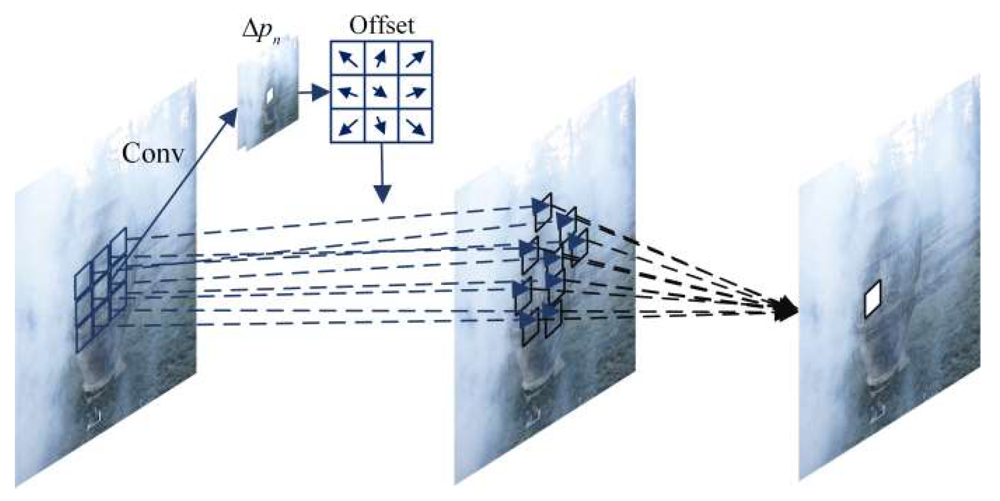
- In most networks, convolution typically uses a fixed-size kernel. When faced with irregular noise such as haze, information cannot be extracted well. In addition, current networks learn the features of non-hazy images, and one limitation of these methods is that they overlook the potential features present in hazy images. Therefore, a key challenge lies in the effective and comprehensive utilization of the information inherent in hazy images.
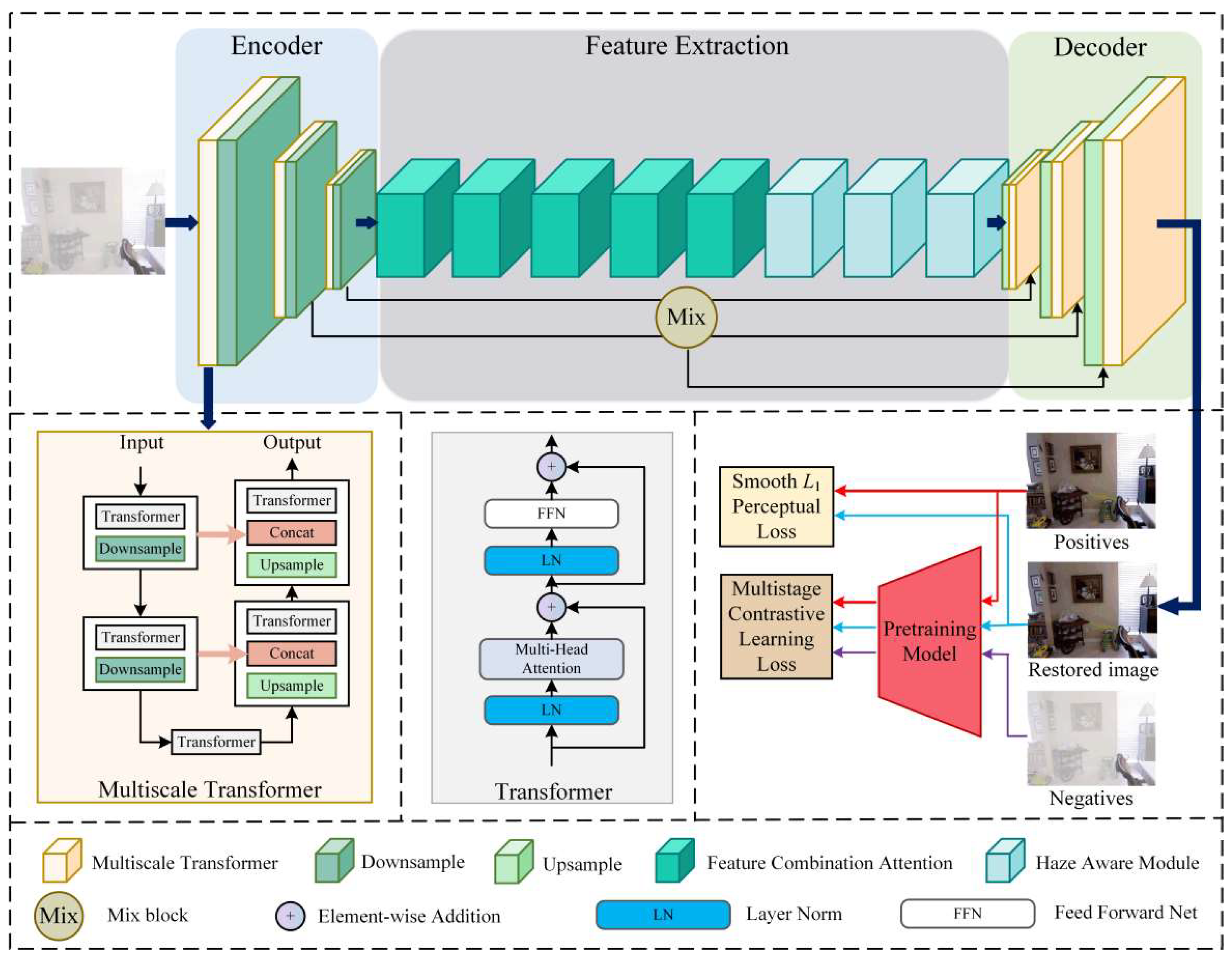
- We propose a multiscale transformer with an encoder–decoder structure, which is connected using residual connections. This structure enables the network to fuse haze information from multiple scales and learn the global information of hazy images.
- We design a haze-aware module and add feature combination attention to the feature extraction, which enables the network to have a more vital transformation ability to fit the feature distribution of the haze.
- We design a novel multistage contrastive learning loss method. By employing different positive and negative sample pairs in the three stages, the network can effectively leverage information from both hazy and non-hazy images to achieve improved recovery consistency.
2. Related Work
2.1. Prior-Based Methods
2.2. Neural Network-Based Methods
3. Proposed Method
3.1. Overview
3.2. Multiscale Transformer
3.3. Feature Extraction
3.3.1. Feature Combination Attention
3.3.2. Haze-Aware Module
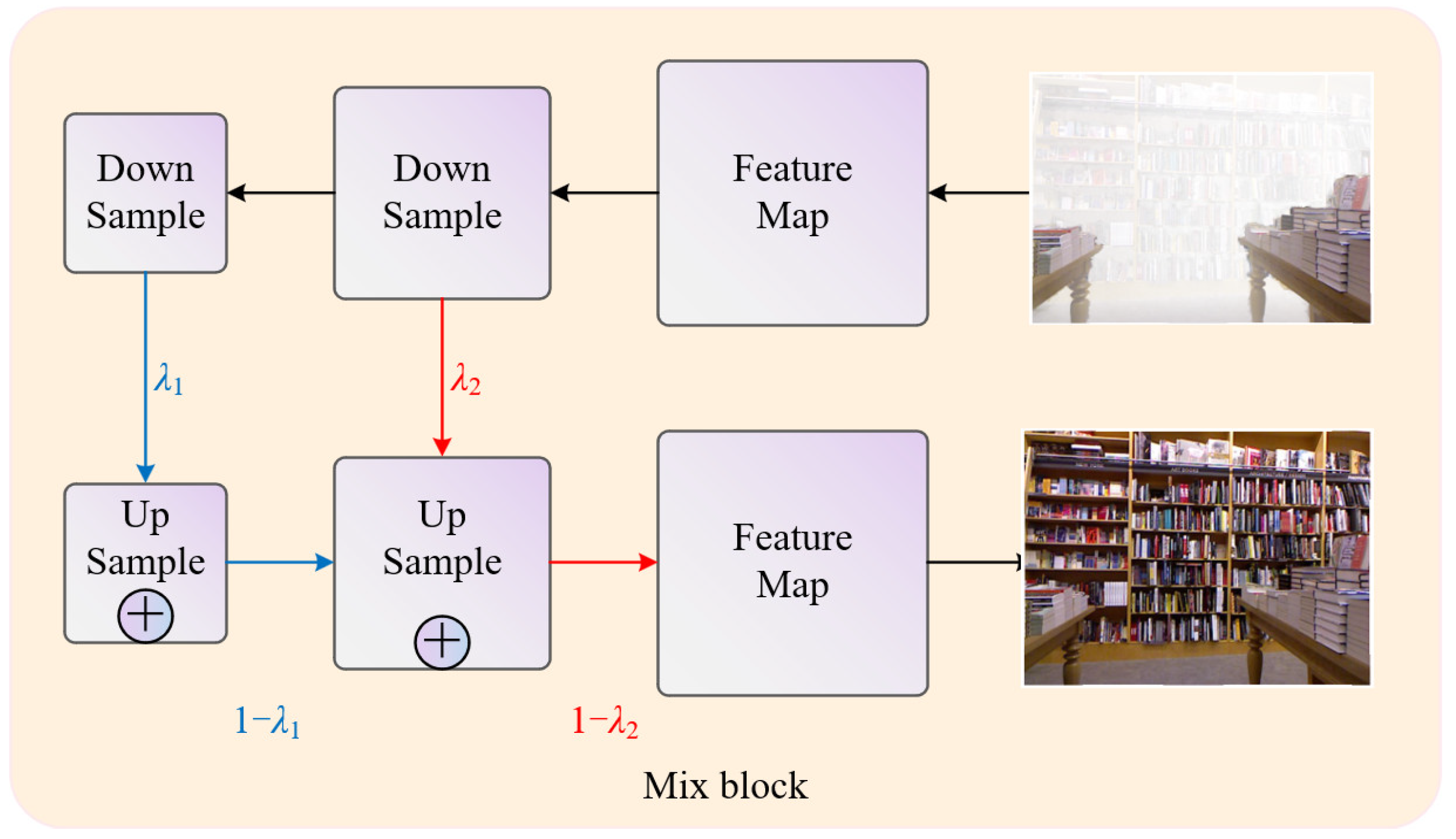
3.3.3. Mixed Block
3.4. Multistage Contrastive Learning Loss
- The first stage uses a piece of the hazy image and a piece of the ground truth image corresponding to this image as positive and negative samples, respectively, to enable the network to better dehaze.
- In the second stage, the positive sample selects another piece of the restored image, and the negative sample selects a piece of the image after downsampling. This selection aims to ensure the consistency of image restoration and avoid haze in different periods.
- In the third stage, we select the real non-hazy image and the hazy image of another image from the dataset as the positive and negative samples, respectively. This means that we want the network to learn more about haze characteristics without paying attention to the image content.
4. Experiments
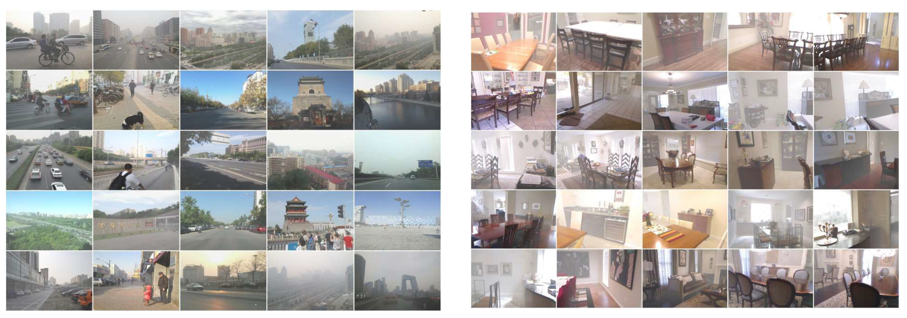
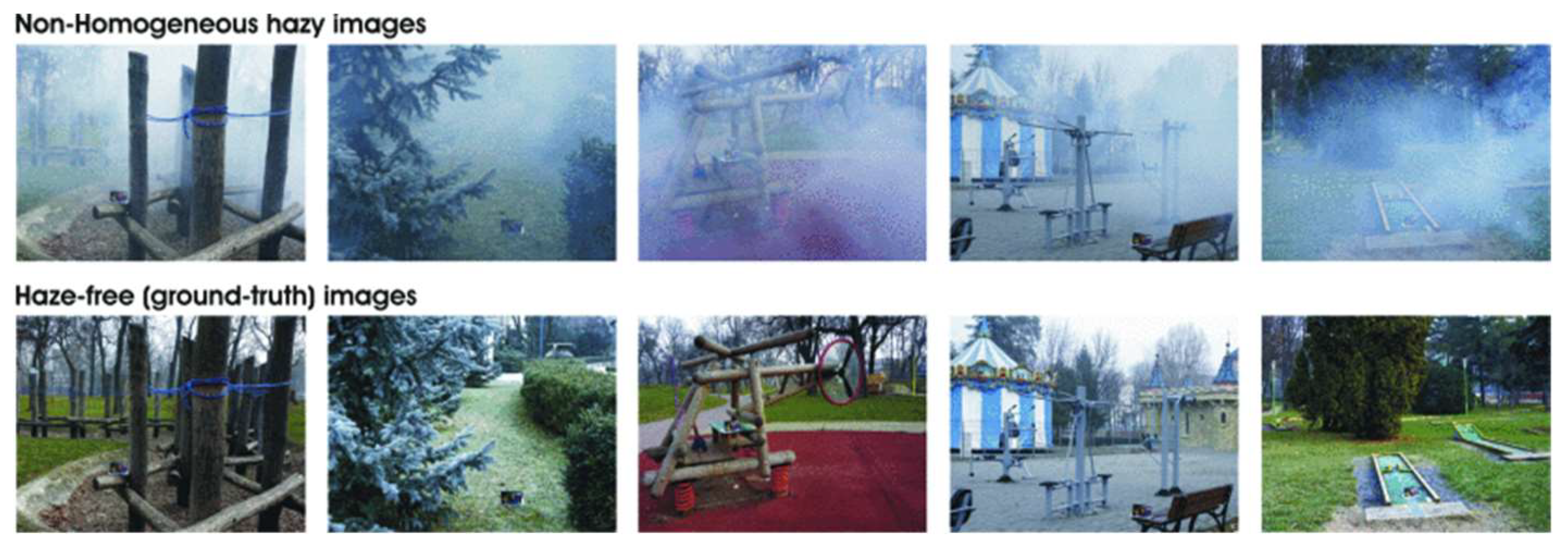
4.1. Datasets
4.2. Comparison Methods and Metrics
4.3. Implementation Details
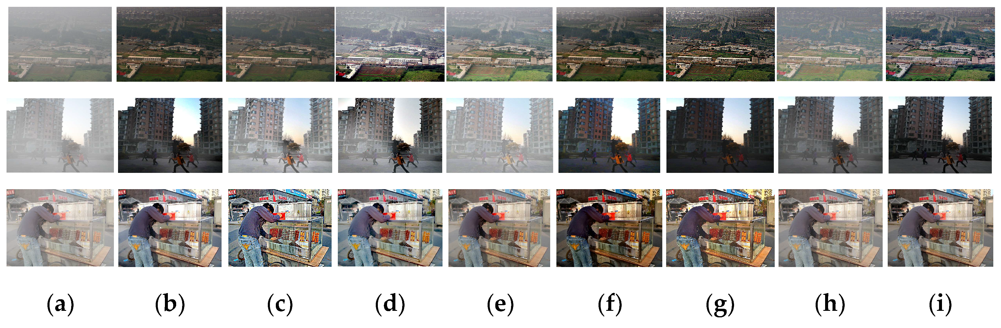
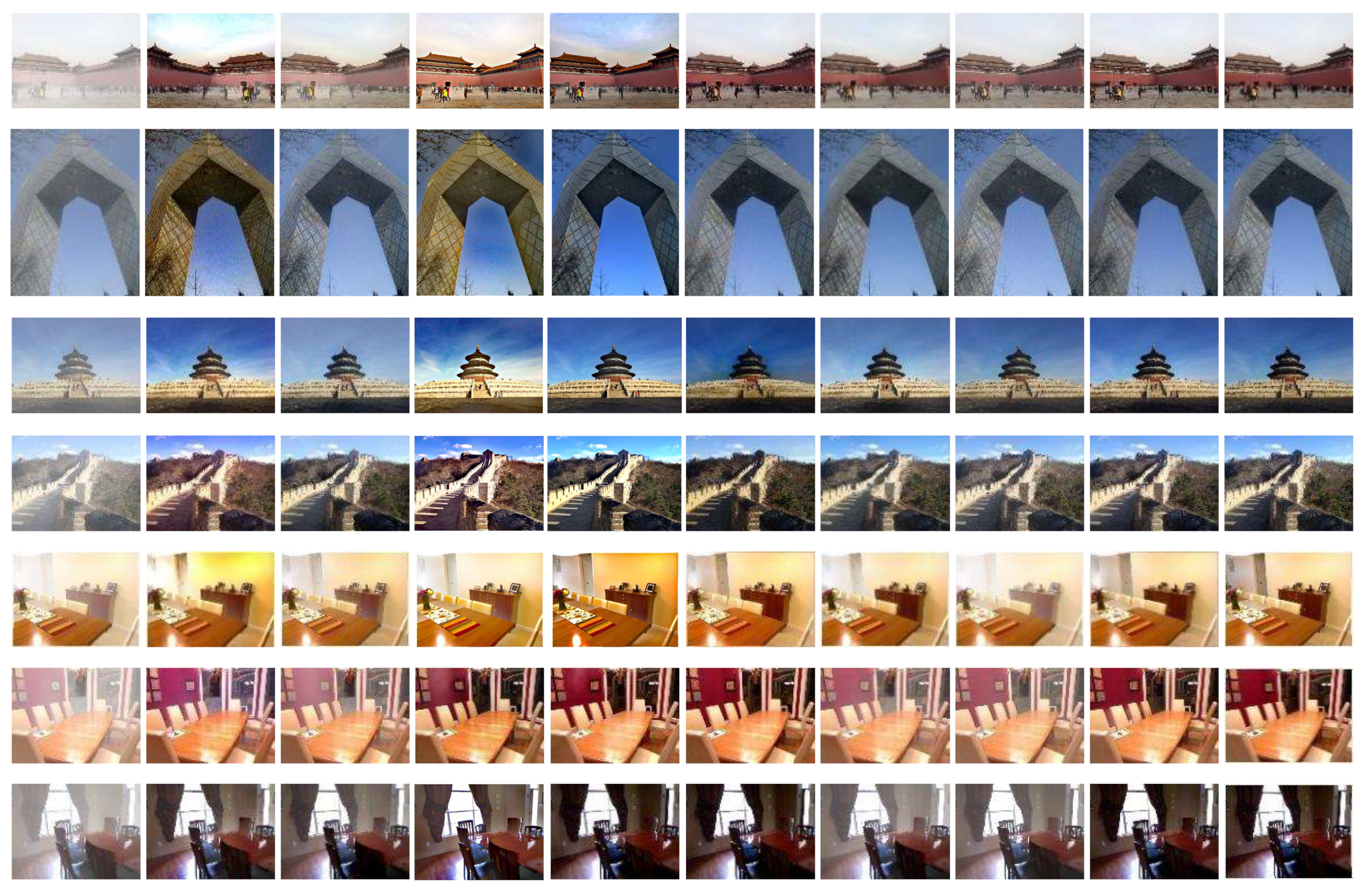
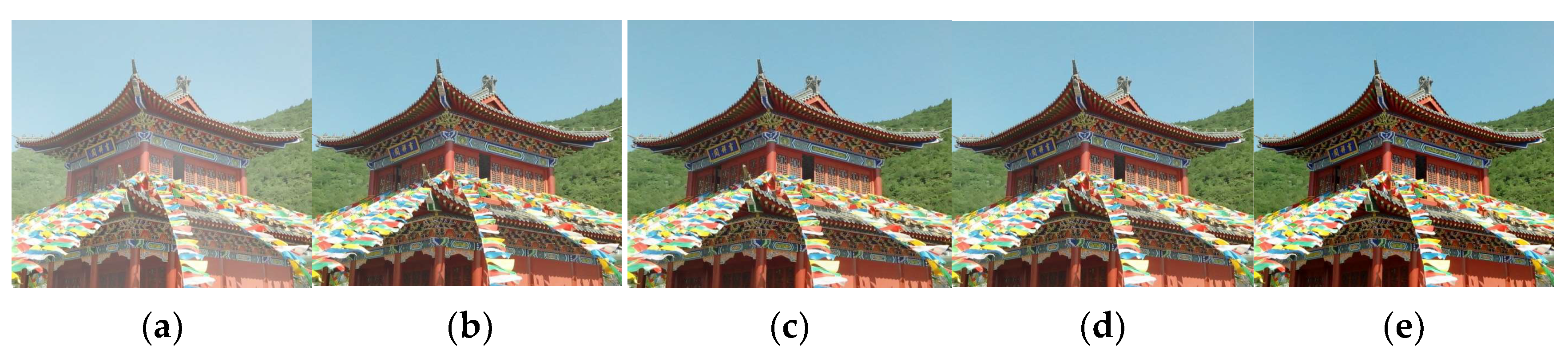
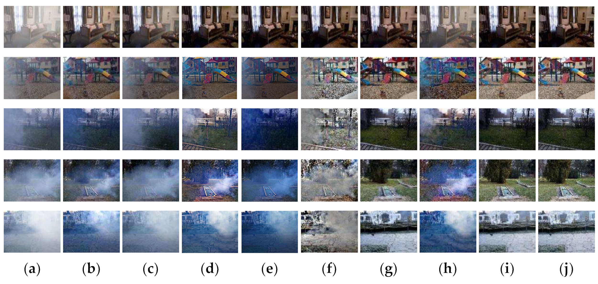
4.4. Image Results Analysis
4.4.1. Qualitative Analysis
4.4.2. Quantitative Analysis
4.5. Ablation Study
5. Conclusions
Author Contributions
Funding
Institutional Review Board Statement
Informed Consent Statement
Data Availability Statement
Conflicts of Interest
References
- Sakaridis, C.; Dai, D.; Hecker, S.; Van Gool, L. Model adaptation with synthetic and real data for semantic dense foggy scene understanding. In Proceedings of the European Conference on Computer Vision (ECCV), Munich, Germany, 8–14 September 2018; pp. 687–704. [Google Scholar]
- Carion, N.; Massa, F.; Synnaeve, G.; Usunier, N.; Kirillov, A.; Zagoruyko, S. End-to-end object detection with transformers. In Proceedings of the European Conference on Computer Vision, Glasgow, UK, 23–28 August 2020; pp. 213–229. [Google Scholar]
- Kumari, A.; Sahoo, S.K. Real time image and video deweathering: The future prospects and possibilities. Optik 2016, 127, 829–839. [Google Scholar] [CrossRef]
- Prakash, A.; Chitta, K.; Geiger, A. Multi-modal fusion transformer for end-to-end autonomous driving. In Proceedings of the IEEE/CVF Conference on Computer Vision and Pattern Recognition, Nashville, TN, USA, 25 June 2021; pp. 7077–7087. [Google Scholar]
- McCartney, E.J. Optics of the Atmosphere: Scattering by Molecules and Particles; John Wiley and Sons, Inc. : New York, NY, USA, 1976. [Google Scholar] [CrossRef]
- Nayar, S.K.; Narasimhan, S.G. Vision in bad weather. In Proceedings of the Seventh IEEE International Conference on Computer Vision, Corfu, Greece, 25 September 1999; pp. 820–827. [Google Scholar]
- Narasimhan, S.G.; Nayar, S.K. Vision and the atmosphere. Int. J. Comput. Vis. 2002, 48, 233–254. [Google Scholar] [CrossRef]
- He, K.; Sun, J.; Tang, X. Single image haze removal using dark channel prior. IEEE Trans. Pattern Anal. Mach. Intell. 2010, 33, 2341–2353. [Google Scholar] [PubMed]
- Berman, D.; Treibitz, T.; Avidan, S. Single image dehazing using haze-lines. IEEE Trans. Pattern Anal. Mach. Intell. 2018, 42, 720–734. [Google Scholar] [CrossRef] [PubMed]
- Ju, M.; Ding, C.; Guo, C.A.; Ren, W.; Tao, D. IDRLP: Image dehazing using region line prior. IEEE Trans. Image Process. 2021, 30, 9043–9057. [Google Scholar] [CrossRef] [PubMed]
- Zhao, X. Single image dehazing using bounded channel difference prior. In Proceedings of the IEEE/CVF Conference on Computer Vision and Pattern Recognition, Nashville, TN, USA, 25 June 2021; pp. 727–735. [Google Scholar]
- Li, Z.; Shu, H.; Zheng, C. Multi-scale single image dehazing using Laplacian and Gaussian pyramids. IEEE Trans. Image Process. 2021, 30, 9270–9279. [Google Scholar] [CrossRef]
- Cai, B.; Xu, X.; Jia, K.; Qing, C.; Tao, D. Dehazenet: An end-to-end system for single image haze removal. IEEE Trans. Image Process. 2016, 25, 5187–5198. [Google Scholar] [CrossRef]
- Lu, H.; Li, Y.; Nakashima, S.; Serikawa, S. Single image dehazing through improved atmospheric light estimation. Multimed. Tools Appl. 2016, 75, 17081–17096. [Google Scholar] [CrossRef]
- Zhang, H.; Patel, V.M. Densely connected pyramid dehazing network. In Proceedings of the IEEE Conference on Computer Vision and Pattern Recognition, Salt Lake City, UT, USA, 18–23 June 2018; pp. 3194–3203. [Google Scholar]
- Li, B.; Peng, X.; Wang, Z.; Xu, J.; Feng, D. Aod-net: All-in-one dehazing network. In Proceedings of the IEEE International Conference on Computer Vision, Venice, Italy, 22–29 October 2017; pp. 4770–4778. [Google Scholar]
- Zhou, C.; Teng, M.; Han, Y.; Xu, C.; Shi, B. Learning to dehaze with polarization. Adv. Neural Inf. Process. Syst. 2021, 34, 11487–11500. [Google Scholar]
- Dong, J.; Pan, J. Physics-based feature dehazing networks. In Proceedings of the Computer Vision–ECCV 2020: 16th European Conference, Glasgow, UK, 23–28 August 2020; pp. 188–204. [Google Scholar]
- Li, R.; Pan, J.; Li, Z.; Tang, J. Single image dehazing via conditional generative adversarial network. In Proceedings of the IEEE Conference on Computer Vision and Pattern Recognition, Salt Lake City, UT, USA, 18–23 June 2018; pp. 8202–8211. [Google Scholar]
- Liu, X.; Ma, Y.; Shi, Z.; Chen, J. Griddehazenet: Attention-based multi-scale network for image dehazing. In Proceedings of the IEEE/CVF International Conference on Computer Vision, Seoul, Republic of Korea, 27 October–2 November 2019; pp. 7314–7323. [Google Scholar]
- Vaswani, A.; Shazeer, N.; Parmar, N.; Uszkoreit, J.; Jones, L.; Gomez, A.N.; Kaiser, Ł.; Polosukhin, I. Attention is all you need. Adv. Neural Inf. Process. Syst. 2017, 30, 5998–6008. [Google Scholar]
- Song, Y.; He, Z.; Qian, H.; Du, X. Vision transformers for single image dehazing. IEEE Trans. Image Process. 2023, 32, 1927–1941. [Google Scholar] [CrossRef] [PubMed]
- Choi, L.K.; You, J.; Bovik, A.C. Referenceless prediction of perceptual fog density and perceptual image defogging. IEEE Trans. Image Process. 2015, 24, 3888–3901. [Google Scholar] [CrossRef]
- Fattal, R. Dehazing using color-lines. ACM Trans. Graph. 2014, 34, 1–14. [Google Scholar] [CrossRef]
- Tan, R.T. Visibility in bad weather from a single image. In Proceedings of the 2008 IEEE Conference on Computer Vision and Pattern Recognition, Anchorage, AK, USA, 24–26 June 2008; pp. 1–8. [Google Scholar]
- Fattal, R. Single image dehazing. ACM Trans. Graph. 2008, 27, 1–9. [Google Scholar] [CrossRef]
- Zhou, J.; Zhou, F. Single image dehazing motivated by Retinex theory. In Proceedings of the 2013 2nd International Symposium on Instrumentation and Measurement, Sensor Network and Automation (IMSNA), Toronto, ON, Canada, 23–24 December 2013; pp. 243–247. [Google Scholar]
- Zhang, Q.; Li, X. Fast image dehazing using guided filter. In Proceedings of the 2015 IEEE 16th International Conference on Communication Technology (ICCT), Hangzhou, China, 18–21 October 2015; pp. 182–185. [Google Scholar]
- Wang, J.; Lu, K.; Xue, J.; He, N.; Shao, L. Single image dehazing based on the physical model and MSRCR algorithm. IEEE Trans. Circuits Syst. Video Technol. 2017, 28, 2190–2199. [Google Scholar] [CrossRef]
- Ma, R.; Hu, H.; Xing, S.; Li, Z. Efficient and fast real-world noisy image denoising by combining pyramid neural network and two-pathway unscented Kalman filter. IEEE Trans. Image Process. 2020, 29, 3927–3940. [Google Scholar] [CrossRef] [PubMed]
- Ren, W.; Liu, S.; Zhang, H.; Pan, J.; Cao, X.; Yang, M.-H. Single image dehazing via multi-scale convolutional neural networks. In Proceedings of the Computer Vision–ECCV 2016: 14th European Conference, Amsterdam, The Netherlands, 11–14 October 2016; pp. 154–169. [Google Scholar]
- Chen, D.; He, M.; Fan, Q.; Liao, J.; Zhang, L.; Hou, D.; Yuan, L.; Hua, G. Gated context aggregation network for image dehazing and deraining. In Proceedings of the 2019 IEEE Winter Conference on Applications of Computer Vision (WACV), Waikoloa Village, HI, USA, 7–11 January 2019; pp. 1375–1383. [Google Scholar]
- Qin, X.; Wang, Z.; Bai, Y.; Xie, X.; Jia, H. FFA-Net: Feature Fusion Attention Network for Single Image Dehazing. In Proceedings of the AAAI Conference on Artificial Intelligence, New York, NY, USA, 7–12 February 2020; pp. 11908–11915. [Google Scholar]
- Tu, Z.; Talebi, H.; Zhang, H.; Yang, F.; Milanfar, P.; Bovik, A.; Li, Y. Maxim: Multi-axis mlp for image processing. In Proceedings of the IEEE/CVF Conference on Computer Vision and Pattern Recognition, New Orleans, LA, USA, 24 June 2022; pp. 5769–5780. [Google Scholar]
- Liu, Y.; Pan, J.; Ren, J.; Su, Z. Learning deep priors for image dehazing. In Proceedings of the IEEE/CVF International Conference on Computer Vision, Seoul, Republic of Korea, 28 October 2019; pp. 2492–2500. [Google Scholar]
- Shao, Y.; Li, L.; Ren, W.; Gao, C.; Sang, N. Domain adaptation for image dehazing. In Proceedings of the IEEE/CVF Conference on Computer Vision and Pattern Recognition, Seattle, WA, USA, 13–19 June 2020; pp. 2808–2817. [Google Scholar]
- Zhang, J.; Ren, W.; Zhang, S.; Zhang, H.; Nie, Y.; Xue, Z.; Cao, X. Hierarchical density-aware dehazing network. IEEE Trans. Cybern. 2021, 52, 11187–11199. [Google Scholar] [CrossRef]
- Zhang, S.; Ren, W.; Tan, X.; Wang, Z.-J.; Liu, Y.; Zhang, J.; Zhang, X.; Cao, X. Semantic-aware dehazing network with adaptive feature fusion. IEEE Trans. Cybern. 2021, 53, 454–467. [Google Scholar] [CrossRef]
- Dong, H.; Pan, J.; Xiang, L.; Hu, Z.; Zhang, X.; Wang, F.; Yang, M.-H. Multi-scale boosted dehazing network with dense feature fusion. In Proceedings of the IEEE/CVF Conference on Computer Vision and Pattern Recognition, Seattle, WA, USA, 13–19 June 2020; pp. 2157–2167. [Google Scholar]
- Chen, Z.; Wang, Y.; Yang, Y.; Liu, D. PSD: Principled synthetic-to-real dehazing guided by physical priors. In Proceedings of the IEEE/CVF Conference on Computer Vision and Pattern Recognition, Nashville, TN, USA, 20–25 June 2021; pp. 7180–7189. [Google Scholar]
- Goodfellow, I.; Pouget-Abadie, J.; Mirza, M.; Xu, B.; Warde-Farley, D.; Ozair, S.; Courville, A.; Bengio, Y. Generative adversarial nets. Adv. Neural Inf. Process. Syst. 2014, 27, 2672–2680. [Google Scholar]
- Zheng, Y.; Zhan, J.; He, S.; Dong, J.; Du, Y. Curricular contrastive regularization for physics-aware single image dehazing. In Proceedings of the IEEE/CVF Conference on Computer Vision and Pattern Recognition, Vancouver, BC, Canada, 17–24 June 2023; pp. 5785–5794. [Google Scholar]
- Zhao, S.; Zhang, L.; Shen, Y.; Zhou, Y. RefineDNet: A weakly supervised refinement framework for single image dehazing. IEEE Trans. Image Process. 2021, 30, 3391–3404. [Google Scholar] [CrossRef]
- Golts, A.; Freedman, D.; Elad, M. Unsupervised single image dehazing using dark channel prior loss. IEEE Trans. Image Process. 2019, 29, 2692–2701. [Google Scholar] [CrossRef] [PubMed]
- Wang, Z.; Cun, X.; Bao, J.; Zhou, W.; Liu, J.; Li, H. Uformer: A general u-shaped transformer for image restoration. In Proceedings of the IEEE/CVF Conference on Computer Vision and Pattern Recognition, New Orleans, LA, USA, 18–24 June 2022; pp. 17683–17693. [Google Scholar]
- Liu, Z.; Lin, Y.; Cao, Y.; Hu, H.; Wei, Y.; Zhang, Z.; Lin, S.; Guo, B. Swin transformer: Hierarchical vision transformer using shifted windows. In Proceedings of the IEEE/CVF International Conference on Computer Vision, Montreal, BC, Canada, 11–17 October 2021; pp. 10012–10022. [Google Scholar]
- Dosovitskiy, A.; Beyer, L.; Kolesnikov, A.; Weissenborn, D.; Zhai, X.; Unterthiner, T. Transformers for image recognition at scale. arXiv 2020, arXiv:2010.11929. [Google Scholar]
- Hu, J.; Shen, L.; Sun, G. Squeeze-and-excitation networks. In Proceedings of the IEEE Conference on Computer Vision and Pattern Recognition, Salt Lake City, UT, USA, 18–23 June 2018; pp. 7132–7141. [Google Scholar]
- Wu, H.; Qu, Y.; Lin, S.; Zhou, J.; Qiao, R.; Zhang, Z.; Xie, Y.; Ma, L. Contrastive learning for compact single image dehazing. In Proceedings of the IEEE/CVF Conference on Computer Vision and Pattern Recognition, Nashville, TN, USA, 19–25 June 2021; pp. 10551–10560. [Google Scholar]
- He, K.; Fan, H.; Wu, Y.; Xie, S.; Girshick, R. Momentum contrast for unsupervised visual representation learning. In Proceedings of the IEEE/CVF Conference on Computer Vision and Pattern Recognition, Seattle, WA, USA, 14–19 June 2020; pp. 9729–9738. [Google Scholar]
- Zeiler, M.D.; Fergus, R. Visualizing and understanding convolutional networks. In Proceedings of the Computer Vision–ECCV 2014: 13th European Conference, Zurich, Switzerland, 6–12 September 2014; pp. 818–833. [Google Scholar]
- Simonyan, K.; Zisserman, A. Very deep convolutional networks for large-scale image recognition. arXiv 2014, arXiv:1409.1556. [Google Scholar]
- Zhu, J.-Y.; Park, T.; Isola, P.; Efros, A.A. Unpaired image-to-image translation using cycle-consistent adversarial networks. In Proceedings of the IEEE International Conference on Computer Vision, Venice, Italy, 22–29 October 2017; pp. 2223–2232. [Google Scholar]
- Li, B.; Ren, W.; Fu, D.; Tao, D.; Feng, D.; Zeng, W.; Wang, Z. Benchmarking single-image dehazing and beyond. IEEE Trans. Image Process. 2018, 28, 492–505. [Google Scholar] [CrossRef] [PubMed]
- Ancuti, C.O.; Ancuti, C.; Timofte, R. NH-HAZE: An image dehazing benchmark with non-homogeneous hazy and haze-free images. In Proceedings of the IEEE/CVF Conference on Computer Vision and Pattern Recognition Workshops, Seattle, WA, USA, 14–19 June 2020; pp. 444–445. [Google Scholar]
- Min, X.; Zhai, G.; Gu, K.; Yang, X.; Guan, X. Objective quality evaluation of dehazed images. IEEE Trans. Intell. Transp. Syst. 2018, 20, 2879–2892. [Google Scholar] [CrossRef]
- Mittal, A.; Soundararajan, R.; Bovik, A.C. Making a “completely blind” image quality analyzer. IEEE Signal Process. Lett. 2012, 20, 209–212. [Google Scholar] [CrossRef]


| Method | Strengths | Weaknesses |
|---|---|---|
| Prior-based method [8,23,24,26,27,28,29,30] | Wide applicability, fast calculation, and good visual effect after restoration. | Unable to remove haze in dense haze areas, resulting in color distortion. |
| Network based on physical models [15,16,31,34,39,42] | Only the parameters related to the physical model need to be learned, and the computational data are limited. After restoration, the haze in the image is basically removed. | For real and complex environments that do not satisfy prior conditions, it is impossible to remove haze, and if errors occur when calculating parameters in the physical model, the errors will accumulate, leading to the loss of information in the restored image. |
| Network based on CNN structure [32,33,34,35,36,37,38] | The CNN structure can learn features well, has a wide range of applicability, and can directly generate haze-free images end-to-end. | CNNs cannot capture the global information of images, and there may be overfitting issues. There is no targeted module for characterizing and learning the irregular noise of haze. |
| Network based on transformer [22,45,46] | Transformer can capture global information of images and has strong parallelism, which is more conducive to network training, and can adapt well to complex images. | Transformer requires more computing resources and can only learn global information at a single scale, making it impossible to transmit at different scales. In addition, the potential information of hazy images is ignored, and there is a lack of modules for learning and fitting haze. |
| CMT-Net (ours) | For hazy areas, haze can be completely removed, and the information from hazy images can be utilized to improve recovery consistency. The restored image is more realistic and natural, while preserving the original scene information and texture details. | The network computing cost is high, and the processing effect for hazy images at night is not good, and the network’s ability is limited by the number of datasets. |
| Block | Layer | Input | Output |
|---|---|---|---|
| Multiscale Transformer | Transformer_1 | C × W × H | C × W × H |
| Downsample_1 | C × W × H | 2C × W/2 × H/2 | |
| Transformer_2 | 2C × W/2 × H/2 | 2C × W/2 × H/2 | |
| Downsample_2 | 2C × W/2 × H/2 | 4C × W/4 × H/4 | |
| Transformer_3 | 4C × W/4 × H/4 | 4C × W/4 × H/4 | |
| Upsample_2 | 4C × W/4 × H/4 | 2C × W/2 × H/2 | |
| Concat_2 | 2C × W/2 × H/2 | 2C × W/2 × H/2 | |
| Transformer_2 | 2C × W/2 × H/2 | 2C × W/2 × H/2 | |
| Upsample_1 | 2C × W/2 × H/2 | C × W × H | |
| Concat_1 | C × W × H | C × W × H | |
| Transformer_1 | C × W × H | C × W × H | |
| Encoder–Decoder | Multiscale Transformer_1 | C × W × H | C × W × H |
| Downsample_1 | C × W × H | 2C × W/2 × H/2 | |
| Multiscale Transformer_2 | 2C × W/2 × H/2 | 2C × W/2 × H/2 | |
| Downsample_2 | 2C × W/2 × H/2 | 4C × W/4 × H/4 | |
| Multiscale Transformer_3 | 4C × W/4 × H/4 | 4C × W/4 × H/4 | |
| Downsample_3 | 4C × W/4 × H/4 | 8C × W/8 × H/8 | |
| Feature Extraction | 8C × W/8 × H/8 | 8C × W/8 × H/8 | |
| Upsample_3 | 8C × W/8 × H/8 | 4C × W/4 × H/4 | |
| Multiscale Transformer_3 | 4C × W/4 × H/4 | 4C × W/4 × H/4 | |
| Upsample_2 | 4C × W/4 × H/4 | 2C × W/2 × H/2 | |
| Multiscale Transformer_2 | 2C × W/2 × H/2 | 2C × W/2 × H/2 | |
| Upsample_1 | 2C × W/2 × H/2 | C × W × H | |
| Multiscale Transformer_1 | C × W × H | C × W × H |
| Method | RESIDE | OTS | SOTS | Param (M) | MACs (G) | Run Time(s) | |||
|---|---|---|---|---|---|---|---|---|---|
| DCP | 44.722 | 4.312 | 14.65 | 0.734 | 15.72 | 0.692 | - | - | 19.36 |
| DCPDN | 50.975 | 4.128 | 21.15 | 0.842 | 18.69 | 0.815 | 66.89 | 0.581 | 24.94 |
| RefineDNet | 51.725 | 3.842 | 26.45 | 0.907 | 18.75 | 0.835 | 65.80 | 26.24 | 0.77 |
| AECRNet | 49.453 | 3.712 | 17.54 | 0.842 | 19.43 | 0.829 | 2.61 | 28.08 | 0.87 |
| Maxim | 66.167 | 3.578 | 28.99 | 0.934 | 20.73 | 0.889 | 14.1 | 216 | 15.53 |
| DehazeFormer | 59.963 | 3.541 | 29.23 | 0.945 | 19.75 | 0.852 | 80.45 | 48.93 | 0.12 |
| C2PNet | 52.735 | 4.072 | 28.75 | 0.929 | 17.86 | 0.781 | 9.23 | 7.17 | 1.23 |
| CMT-Net | 63.452 | 3.501 | 30.34 | 0.958 | 21.85 | 0.907 | 39.45 | 34.16 | 1.56 |
| Method | NH-HAZE | Thin Haze | Dense Haze | Run Time(s) | |||
|---|---|---|---|---|---|---|---|
| DCP | 35.87 | 6.154 | 14.94 | 0.713 | 13.59 | 0.531 | 22.61 |
| DCPDN | 30.24 | 6.231 | 13.82 | 0.597 | 11.79 | 0.422 | 25.13 |
| RefineDNet | 33.15 | 6.638 | 11.58 | 0.624 | 14.75 | 0.529 | 0.77 |
| AECRNet | 36.79 | 5.759 | 16.29 | 0.741 | 13.96 | 0.546 | 0.943 |
| Maxim | 32.06 | 5.724 | 14.90 | 0.697 | 11.66 | 0.413 | 17.45 |
| DehazeFormer | 42.26 | 4.956 | 27.89 | 0.902 | 26.73 | 0.807 | 0.15 |
| C2PNet | 38.91 | 5.687 | 14.56 | 0.682 | 11.73 | 0.438 | 1.37 |
| CMT-Net | 45.72 | 4.764 | 28.11 | 0.923 | 26.98 | 0.854 | 1.43 |
| Model | PSNR | SSIM | Param (M) | MACs (G) |
|---|---|---|---|---|
| Base | 24.75 | 0.885 | 0.956 | 21.54 |
| Base + HAM +MB | 26.63 | 0.902 | 2.611 | 22.21 |
| Base + HAM + MB + MT | 29.91 | 0.937 | 26.75 | 28.93 |
| Base + HAM + MB + MT + MCLL | 30.42 | 0.949 | 41.17 | 30.52 |
| Method | PSNR | SSIM |
|---|---|---|
| GCANet | 2.35) | 0.037) |
| C2PNet | 1.21) | 0.021) |
| DCPDN | 0.96) | 0.014) |
| Method | PSNR | SSIM |
|---|---|---|
| DCPDN | 0.35) | 0.018) |
| GridDehazeNet | 0.41) | 0.011) |
| FFA-Net | 0.66) | 0.024) |
Disclaimer/Publisher’s Note: The statements, opinions and data contained in all publications are solely those of the individual author(s) and contributor(s) and not of MDPI and/or the editor(s). MDPI and/or the editor(s) disclaim responsibility for any injury to people or property resulting from any ideas, methods, instructions or products referred to in the content. |
© 2024 by the authors. Licensee MDPI, Basel, Switzerland. This article is an open access article distributed under the terms and conditions of the Creative Commons Attribution (CC BY) license (https://creativecommons.org/licenses/by/4.0/).
Share and Cite
Chen, J.; Zhao, G. Contrastive Multiscale Transformer for Image Dehazing. Sensors 2024, 24, 2041. https://doi.org/10.3390/s24072041
Chen J, Zhao G. Contrastive Multiscale Transformer for Image Dehazing. Sensors. 2024; 24(7):2041. https://doi.org/10.3390/s24072041
Chicago/Turabian StyleChen, Jiawei, and Guanghui Zhao. 2024. "Contrastive Multiscale Transformer for Image Dehazing" Sensors 24, no. 7: 2041. https://doi.org/10.3390/s24072041
APA StyleChen, J., & Zhao, G. (2024). Contrastive Multiscale Transformer for Image Dehazing. Sensors, 24(7), 2041. https://doi.org/10.3390/s24072041