
Decoupling and Parameter Extraction Methods for Conical Micro-Motion Object Based on FMCW Lidar

 ,
,
Abstract
1. Introduction
2. Analysis of One-Dimensional Range Profile of Cone Based on FMCW Lidar
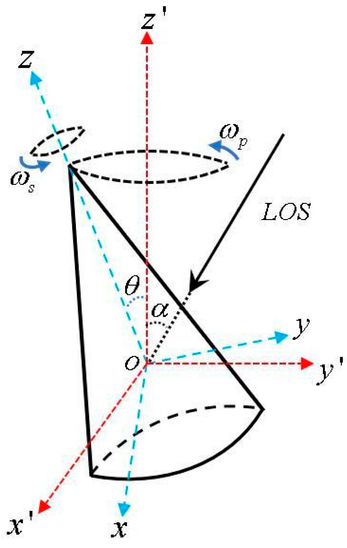
2.1. Dynamic Model Analysis of Precession Cone
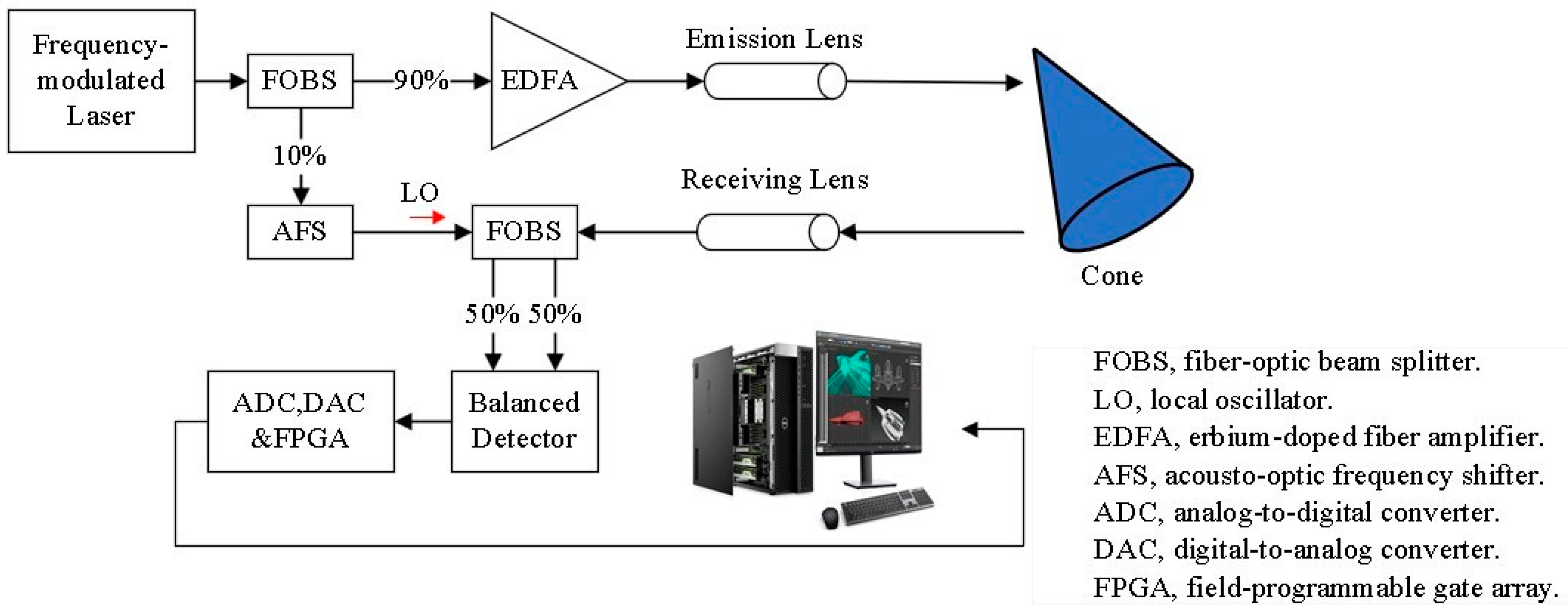
2.2. FMCW Lidar for One-Dimensional Range Profile of Cone
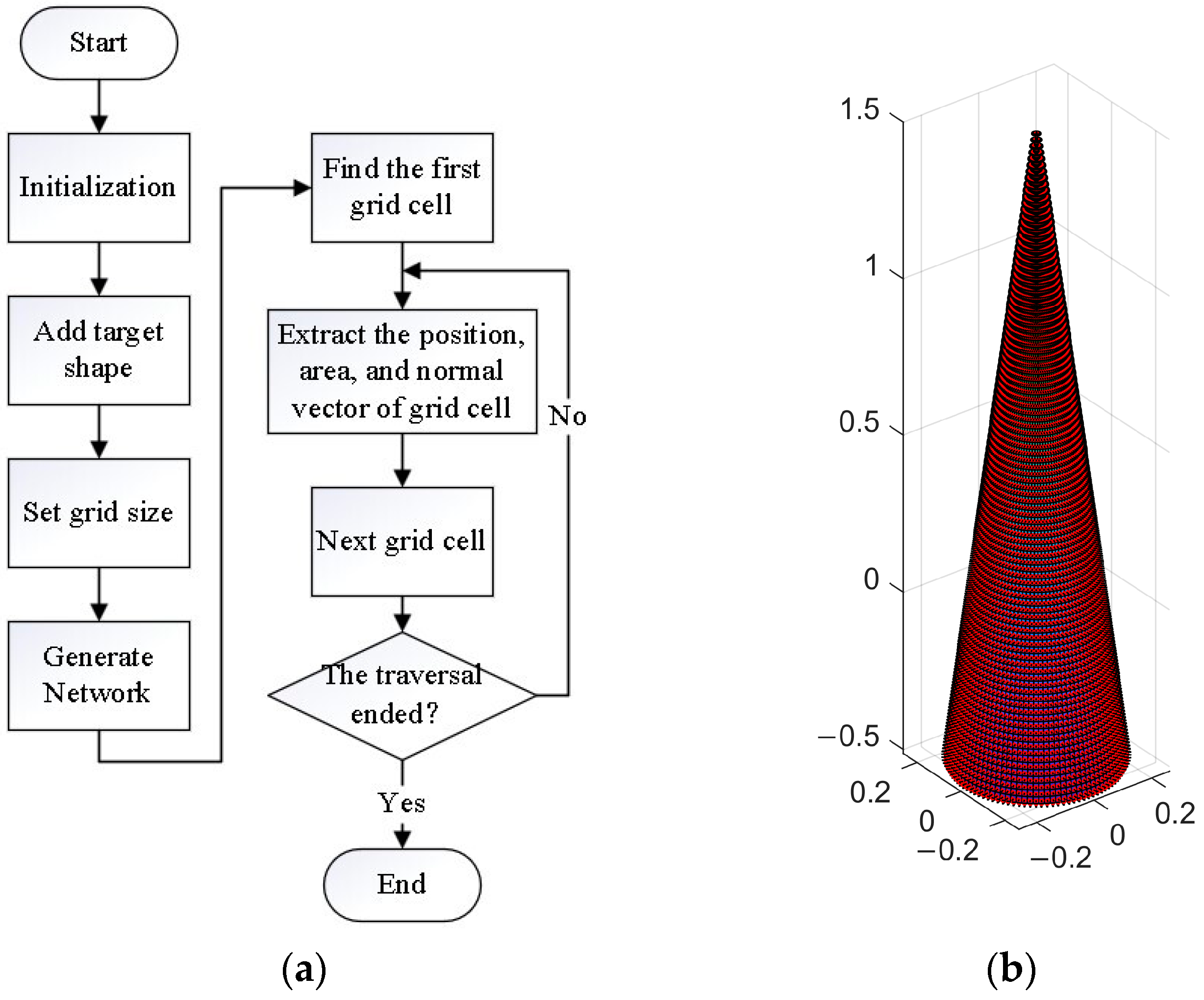
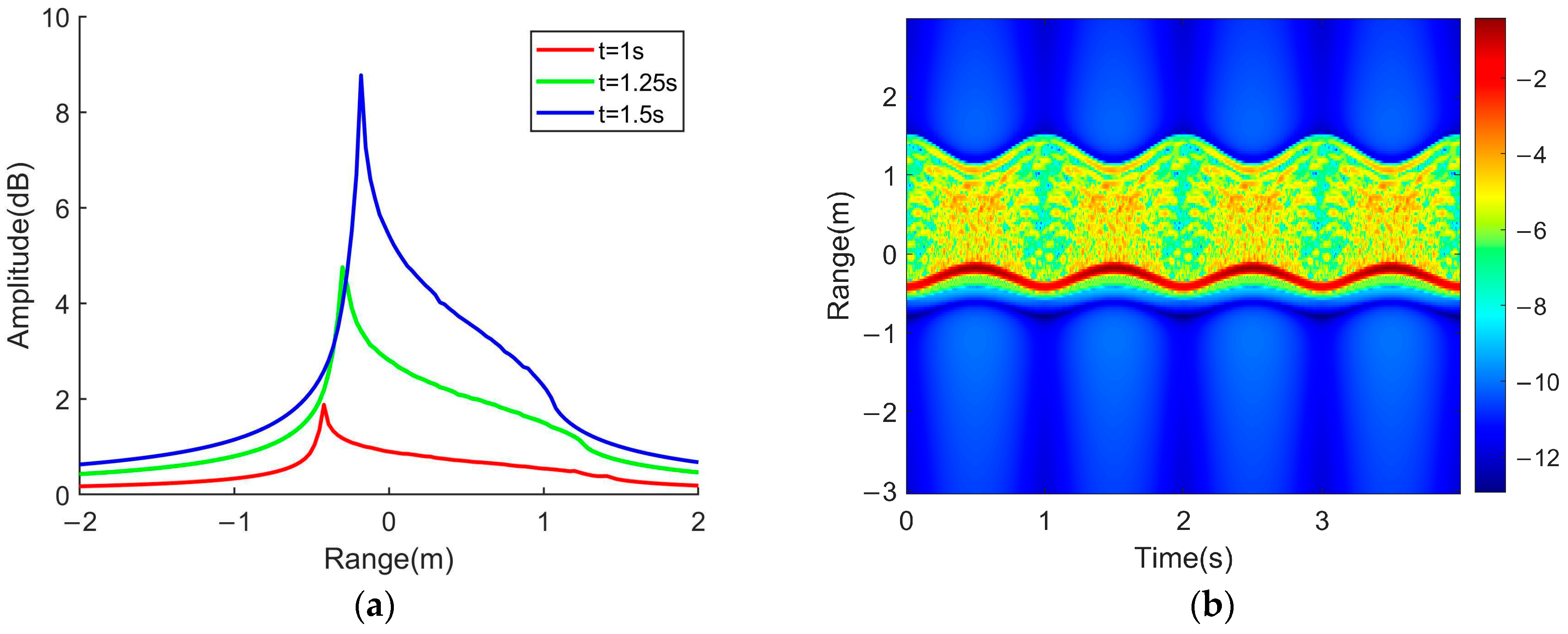
2.3. Simulation Analysis of One-Dimensional Range Profile
3. Analysis of Parameter Decoupling and Extraction Based on Micro-Doppler Time–Frequency Spectrum and Range Profile
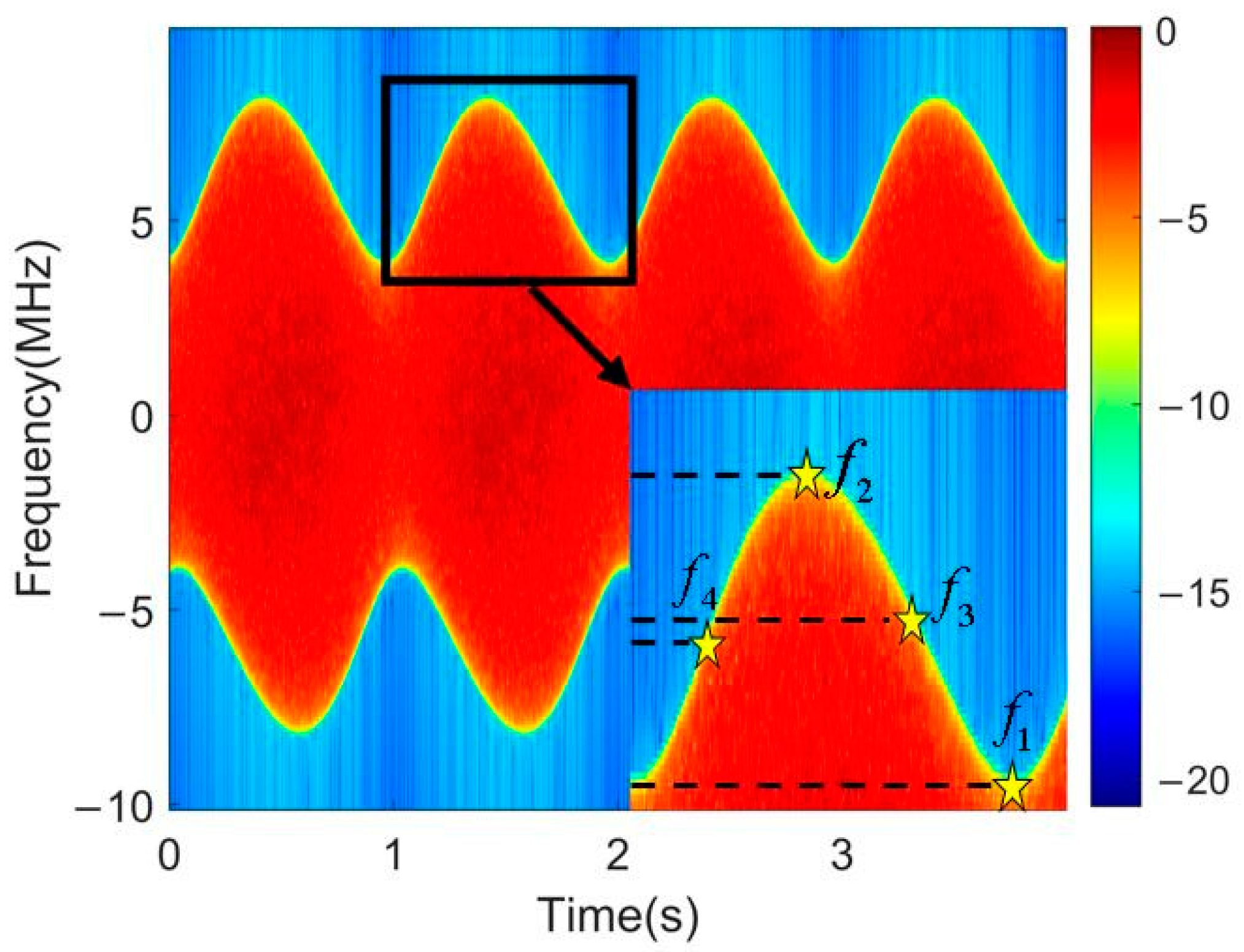
3.1. Acquisition and Simulation of Micro-Doppler Frequency Spectrum for the Micro-Motion Cone
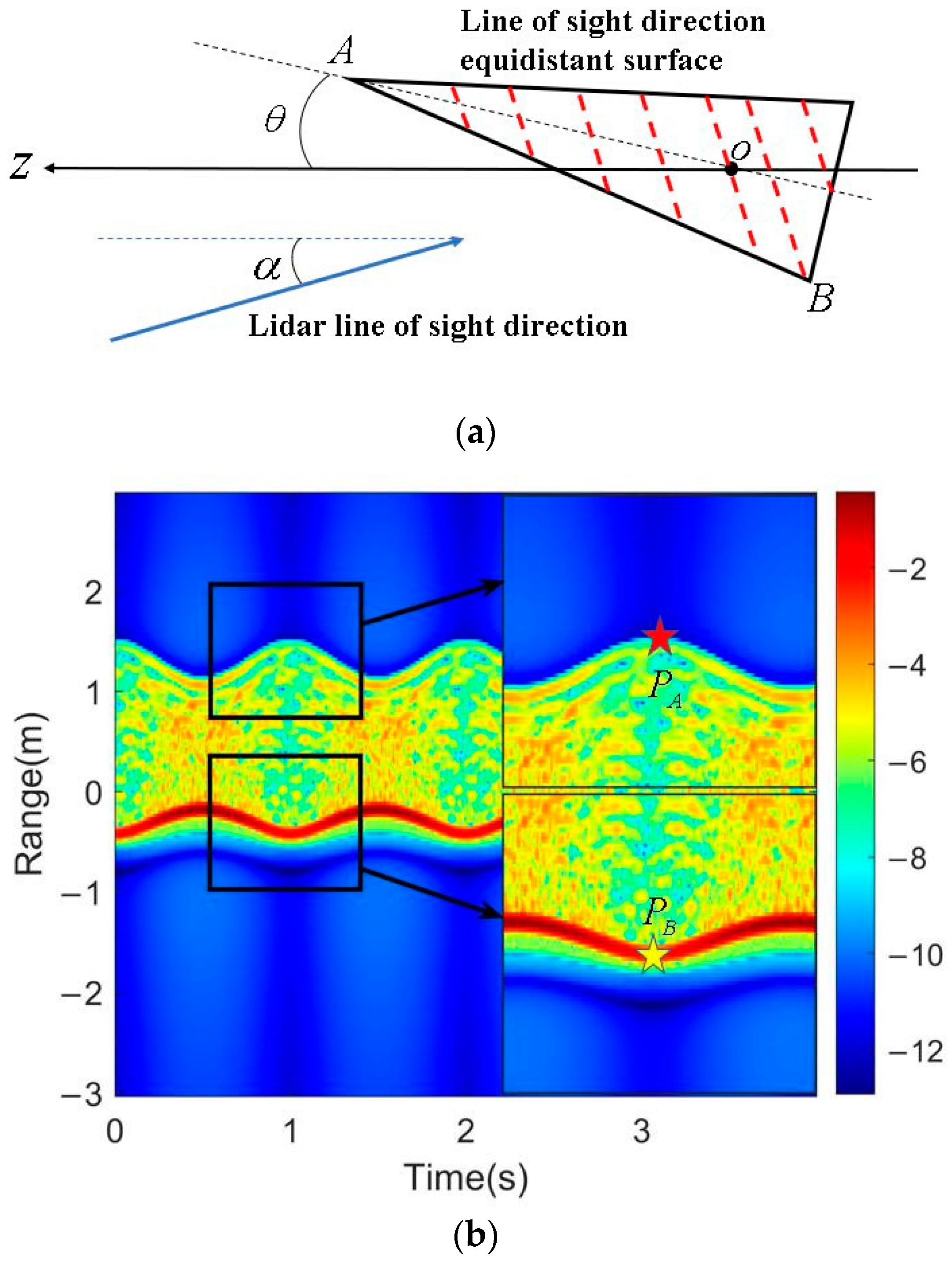
3.2. Parameter Extraction and Analysis of Range Profile for the Micro-Motion Cone
4. Simulation Verification of Conical Micro-Motion Parameter Extraction
5. Conclusions
Author Contributions
Funding
Institutional Review Board Statement
Informed Consent Statement
Data Availability Statement
Conflicts of Interest
References
- Zhou, Y.; Chen, Y.; Zhao, H.; Jamet, C.; Dionisi, D.; Chami, M.; Girolamo, P.D.; Churnside, J.; Malinka, A.; Zhao, H.; et al. Shipborne Oceanic High-Spectral-Resolution Lidar for Accurate Estimation of Seawater Depth-Resolved Optical Properties. Light Sci. Appl. 2022, 11, 261. [Google Scholar] [CrossRef]
- Yalagala, B.P.; Dahiya, A.S.; Dahiya, R. ZnO nanowires based degradable high-performance photodetectors for eco-friendly green electronics. Opto-Electron. Adv. 2023, 6, 220020. [Google Scholar] [CrossRef]
- Vandersmissen, B.; Knudde, N.; Jalalvand, A.; Couckuyt, I.; Bourdoux, A.; De Neve, W.; Dhaene, T. Indoor Person Identification Using a Low-Power FMCW Radar. IEEE Trans. Geosci. Remote Sens. 2018, 56, 3941–3952. [Google Scholar] [CrossRef]
- Kim, Y.; Moon, T. Human Detection and Activity Classification Based on Micro-Doppler Signatures Using Deep Convolutional Neural Networks. IEEE Geosci. Remote Sens. Lett. 2016, 13, 8–12. [Google Scholar] [CrossRef]
- Gurbuz, S.Z.; Amin, M.G. Radar-Based Human-Motion Recognition with Deep Learning: Promising Applications for Indoor Monitoring. IEEE Signal Process. Mag. 2019, 36, 16–28. [Google Scholar] [CrossRef]
- He, X.; Zhang, Y.; Dong, X. Extraction of Human Limbs Based on Micro-Doppler-Range Trajectories Using Wideband Interferometric Radar. Sensors 2023, 23, 7544. [Google Scholar] [CrossRef]
- Zhang, Y.; Li, D.; Han, Y.; Yang, Z.; Dai, X.; Guo, X.; Zhang, J. A New Estimation Method for Rotor Size of UAV Based on Peak Time-Shift Effect in Micro-Doppler Lidar. Front. Phys. 2022, 10, 865240. [Google Scholar] [CrossRef]
- Fan, S.; Wu, Z.; Xu, W.; Zhu, J.; Tu, G. Micro-Doppler Signature Detection and Recognition of UAVs Based on OMP Algorithm. Sensors 2023, 23, 7922. [Google Scholar] [CrossRef] [PubMed]
- Liu, J.; Xiong, W.; Bai, L.; Xia, Y.; Huang, T.; Ouyang, W.; Zhu, B. Deep Instance Segmentation with Automotive Radar Detection Points. IEEE Trans. Intell. Veh. 2023, 8, 84–94. [Google Scholar] [CrossRef]
- Liu, Y.; Qiao, S.; Fang, C.; He, Y.; Sun, H.; Liu, J.; Ma, Y. A highly sensitive LITES sensor based on a multi-pass cell with dense spot pattern and a novel quartz tuning fork with low frequency. Opto-Electron. Adv. 2024, 7, 230230. [Google Scholar] [CrossRef]
- Rahman, S.; Robertson, D.A. Radar Micro-Doppler Signatures of Drones and Birds at K-band and W-band. Sci. Rep. 2018, 8, 17396. [Google Scholar] [CrossRef]
- Chen, V.C.; Li, F.; Ho, S.S.; Wechsler, H. Analysis of Micro-Doppler Signatures. IEE Proc. Radar Sonar Navig. 2003, 150, 271–276. [Google Scholar] [CrossRef]
- Chen, V.C. Analysis of Radar Micro-Doppler with Time-Frequency Transform. In Proceedings of the Tenth IEEE Workshop on Statistical Signal and Array Processing, Pocono Manor, PA, USA, 16 August 2000; pp. 463–466. [Google Scholar] [CrossRef]
- Wang, Z.; Luo, Y.; Li, K.; Yuan, H.; Zhang, Q. Micro-Doppler Parameters Extraction of Precession Cone-Shaped Targets Based on Rotating Antenna. Remote Sens. 2022, 14, 2549. [Google Scholar] [CrossRef]
- Yu, Z.; Chen, Z.; Zhang, L.R.; Xiao, J.G. Micro-Doppler Curves Extraction and Parameters Estimation for Cone-Shaped Target with Occlusion Effect. IEEE Sens. J. 2018, 18, 2892–2902. [Google Scholar]
- Qin, X.; Deng, B.; Wang, H. Micro-Doppler Feature Extraction of Rotating Structures of Aircraft Targets with Terahertz Radar. Remote Sens. 2022, 14, 3856. [Google Scholar] [CrossRef]
- Wang, Y.; Liu, K.; Liu, H.; Wang, J.; Cheng, Y. Detection of Rotational Object in Arbitrary Position Using Vortex Electromagnetic Waves. IEEE Sens. J. 2021, 21, 4989–4994. [Google Scholar] [CrossRef]
- Li, G.; Varshney, P.K. Micro-Doppler Parameter Estimation Via Parametric Sparse Representation and Pruned Orthogonal Matching Pursuit. IEEE J. Sel. Top. Appl. Earth Obs. Remote Sens. 2014, 7, 4937–4948. [Google Scholar] [CrossRef]
- Liang, Y.; Zhang, Q.; Luo, Y.; Bai, Y.; Chen, Y. Micro-Doppler Features Analysis and Extraction of Vibrating Target in FMCW SAR Based on Slow Time Envelope Signatures. IEEE Geosci. Remote Sens. Lett. 2015, 12, 2041–2045. [Google Scholar] [CrossRef]
- Li, Y.; Wu, Z.; Gong, Y.; Zhang, G.; Wang, M. Laser One-Dimensional Range Profile. Acta Oceanol. Sin. 2010, 59, 6988–6993. [Google Scholar]
- Xie, Y.; Hong, S.; Yan, H.; Zhang, C.; Zhang, L.; Zhuang, L.; Dai, D. Low-Loss Chip-Scale Programmable Silicon Photonic Processor. Opto-Electron. Adv. 2023, 6, 220030. [Google Scholar] [CrossRef]
- Bu, L.; Zhu, Y.; Chen, Y.; Song, X.; Yang, Y.; Zang, Y. Micro-Motion Parameter Extraction of Rotating Target Based on Vortex Electromagnetic Wave Radar. Remote Sens. 2022, 14, 5908. [Google Scholar] [CrossRef]
- Zhao, Y.; Yang, Y.; Jiang, L.; Yang, S.; Lian, D.; Yang, Y. Design and Analysis of VCSEL Pulse Lidar Surge Current Suppression Method. Flight Control. Detect. 2022, 5, 49–54. [Google Scholar]
- Kumari, A.; Kumar, A.; Reddy, G.S.T. Performance Analysis of The Coherent FMCW Photonic Radar System under The Influence of Solar Noise. Front. Phys. 2023, 11, 1215160. [Google Scholar] [CrossRef]
- Erdogan, A.Y.; Gulum, T.O.; Durak-Ata, L.; Yildirim, T.; Pace, P.E. FMCW Signal Detection and Parameter Extraction by Cross Wigner–Hough Transform. IEEE Trans. Aerosp. Electron. Syst. 2017, 53, 334–344. [Google Scholar] [CrossRef]
- Lee, J.G. A Study on Estimation of a Beat Spectrum in a FMCW Radar. J. Korean Inst. Inf. Commun. Eng. 2009, 13, 2511–2517. [Google Scholar]
- Peter, S.; Reddy, V.V. Extraction and Analysis of Micro-Doppler Signature in FMCW Radar. In Proceedings of the IEEE Radar Conference (RadarConf 21), Atlanta, GA, USA, 7–14 May 2021; pp. 1–6. [Google Scholar] [CrossRef]
- Elghandour, A.H.; Chen, D.R. Modeling and Comparative Study of Various Detection Techniques for FMCW Lidar Using Optisystem. In Proceedings of the International Symposium on Photoelectronic Detection and Imaging 2013: Laser Sensing and Imaging and Applications, Beijing, China, 25–27 June 2013; p. 890529. [Google Scholar] [CrossRef]
- Yang, F.; Qiu, Z.; Li, S. Research on High-Precision Laser Speed and Distance Measurement System Based on Pseudo-Random Code Phase Modulation and Heterodyne Detection. Flight Control. Detect. 2019, 2, 43–48. [Google Scholar]
- Huang, B.; Ma, C. A Shamanskii-Like Self-Adaptive Levenberg–Marquardt Method for Nonlinear Equations. Comput. Math. Appl. 2019, 77, 357–373. [Google Scholar] [CrossRef]
- Myttenaere, A.D.; Golden, B.; Grand, B.L.; Rossi, F. Mean Absolute Percentage Error for Regression Models. Neurocomputing 2016, 192, 38–48. [Google Scholar] [CrossRef]


| Conical Precession Parameters | FMCW Lidar Transmission Parameters | ||
|---|---|---|---|
| Sweep bandwidth B | 5 GHz | ||
| Sweep period T | 10 μs | ||
| Precession angle θ | 15° | Transmit carrier frequency f0 | 2.82 × 10¹⁴ Hz |
| Lidar line of sight angle | 30° | Detection time t | 4 s |
| Precession frequency | 1 Hz | Carrier wavelength λ | 1064 nm |
| Spin frequency W | 3 Hz | Output power | 300 mW |
| CW radiation line width | 10 kHz | ||
| Output beam quality | 1.2 M2 | ||
| Half beam divergence | 0.019° | ||
| Parameters | Values | |
|---|---|---|
| Cone | cone height h | 2 m |
| height of gravity center d | 0.5 m | |
| bottom radius ρ | 0.25 m | |
| precession angle | 15° | |
| precession frequency | 2 Hz | |
| spin frequency W | 5 Hz | |
| Lidar | sweep bandwidth B | 5 GHz |
| sweep period T | 10 μs | |
| carrier frequency f0 | 2.82 × 10¹⁴ Hz | |
| detection time t | 4 s |
| α (°) | h (m) | d (m) | ρ (m) | W (Hz) | θ (°) |
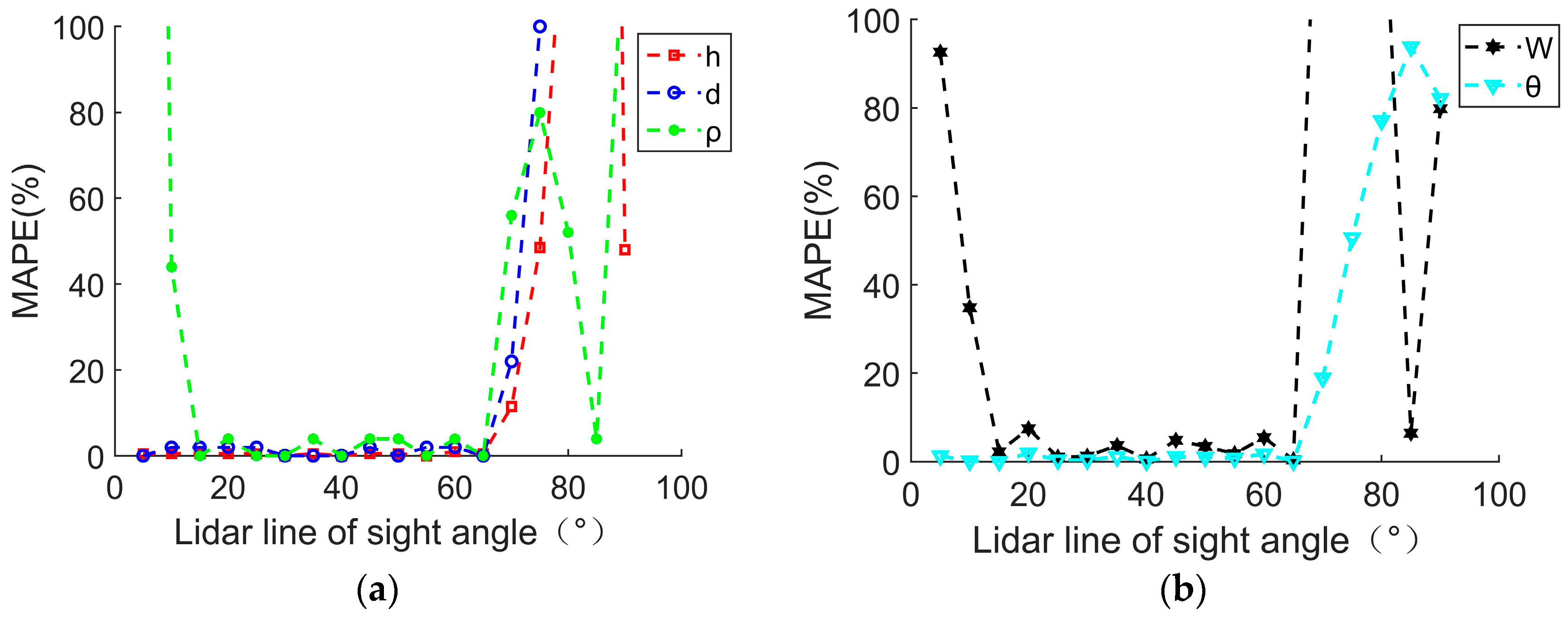
|---|---|---|---|---|---|
| 5 | 2.01 | 0.50 | 1.58 | 0.37 | 14.81 |
| 10 | 1.99 | 0.49 | 0.36 | 3.26 | 15.02 |
| 15 | 2.01 | 0.51 | 0.25 | 5.11 | 15.01 |
| 20 | 2.01 | 0.51 | 0.24 | 5.37 | 14.72 |
| 25 | 1.99 | 0.49 | 0.25 | 4.95 | 15.06 |
| 30 | 2.00 | 0.50 | 0.25 | 4.94 | 15.06 |
| 35 | 1.99 | 0.50 | 0.26 | 4.82 | 15.17 |
| 40 | 2.00 | 0.50 | 0.25 | 4.97 | 15.02 |
| 45 | 1.99 | 0.51 | 0.24 | 5.24 | 14.83 |
| 50 | 1.99 | 0.50 | 0.26 | 4.83 | 15.15 |
| 55 | 2.00 | 0.49 | 0.25 | 4.91 | 15.12 |
| 60 | 1.98 | 0.49 | 0.26 | 4.73 | 15.25 |
| 65 | 1.99 | 0.50 | 0.25 | 5.02 | 14.98 |
| 70 | 2.23 | 0.61 | 0.11 | 13.72 | 12.17 |
| 75 | 2.97 | 1.00 | 0.05 | 30.48 | 7.41 |
| 80 | 4.87 | 2.16 | 0.12 | 11.99 | 3.44 |
| 85 | 12.89 | 7.95 | 0.24 | 5.32 | 0.93 |
| 90 | 2.96 | 2.75 | 0.57 | 1.01 | 2.69 |
| ω (Hz) | h (m) | d (m) | ρ (m) | W (Hz) | θ (°) |
|---|---|---|---|---|---|
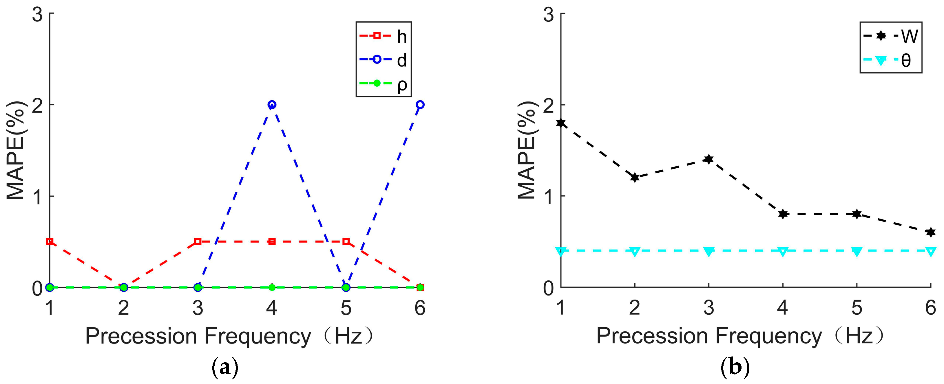
| 1 | 1.99 | 0.50 | 0.25 | 4.91 | 15.06 |
| 2 | 2.00 | 0.50 | 0.25 | 4.94 | 15.06 |
| 3 | 1.99 | 0.50 | 0.25 | 4.93 | 15.06 |
| 4 | 1.99 | 0.49 | 0.25 | 4.96 | 15.06 |
| 5 | 1.99 | 0.50 | 0.25 | 4.96 | 15.06 |
| 6 | 2.00 | 0.49 | 0.25 | 4.97 | 15.06 |
Disclaimer/Publisher’s Note: The statements, opinions and data contained in all publications are solely those of the individual author(s) and contributor(s) and not of MDPI and/or the editor(s). MDPI and/or the editor(s) disclaim responsibility for any injury to people or property resulting from any ideas, methods, instructions or products referred to in the content. |
© 2024 by the authors. Licensee MDPI, Basel, Switzerland. This article is an open access article distributed under the terms and conditions of the Creative Commons Attribution (CC BY) license (https://creativecommons.org/licenses/by/4.0/).
Share and Cite
Yang, Z.; Yang, Y.; Liu, M.; Wei, Y.; Zhang, Y.; Zhang, J.; Liu, X.; Dai, X. Decoupling and Parameter Extraction Methods for Conical Micro-Motion Object Based on FMCW Lidar. Sensors 2024, 24, 1832. https://doi.org/10.3390/s24061832
Yang Z, Yang Y, Liu M, Wei Y, Zhang Y, Zhang J, Liu X, Dai X. Decoupling and Parameter Extraction Methods for Conical Micro-Motion Object Based on FMCW Lidar. Sensors. 2024; 24(6):1832. https://doi.org/10.3390/s24061832
Chicago/Turabian StyleYang, Zhen, Yufan Yang, Manguo Liu, Yuan Wei, Yong Zhang, Jianlong Zhang, Xue Liu, and Xin Dai. 2024. "Decoupling and Parameter Extraction Methods for Conical Micro-Motion Object Based on FMCW Lidar" Sensors 24, no. 6: 1832. https://doi.org/10.3390/s24061832
APA StyleYang, Z., Yang, Y., Liu, M., Wei, Y., Zhang, Y., Zhang, J., Liu, X., & Dai, X. (2024). Decoupling and Parameter Extraction Methods for Conical Micro-Motion Object Based on FMCW Lidar. Sensors, 24(6), 1832. https://doi.org/10.3390/s24061832