
Energy-Efficient Collision-Free Machine/AGV Scheduling Using Vehicle Edge Intelligence


Abstract
1. Introduction
2. Background
2.1. Collision Avoidance in Machine/AGV Systems
2.2. Energy Efficiency in Multiple AGVs
2.3. Research Gap
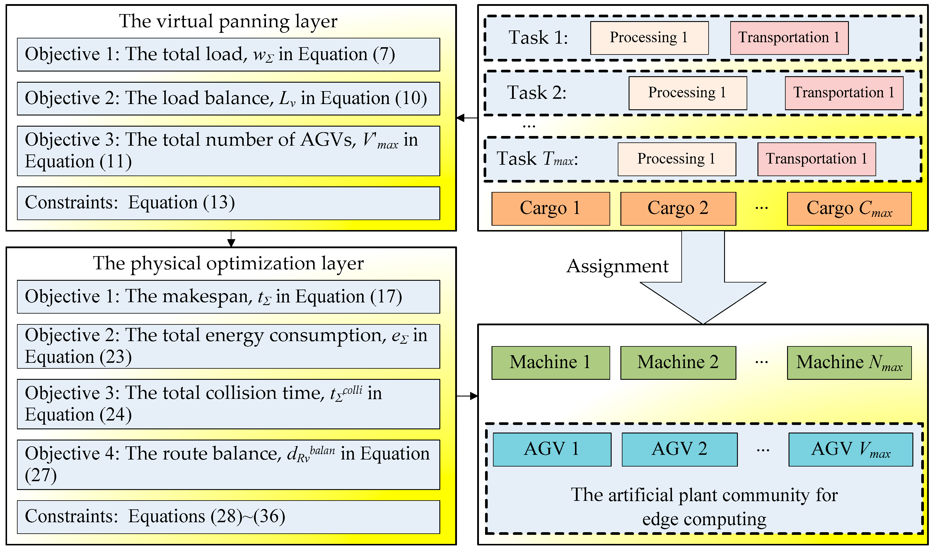
3. A VEI-Based Architecture for the Machine/AGV System
3.1. Characteristics of the VEI Architecture
3.2. The State Transition Diagram for the VPL
- New: This is the first state. If a task requests a machine/AGV, it will be created at first and will wait for an assignment;
- Ready: If a new task is assigned to an idle machine/AGV, it will be ready before performing a task. Then, the machine/AGV is occupied by the task and cannot be used for other purposes;
- Performing: If a task that is ready is scheduled, then the task can be performed on a machine/AGV;
- Waiting: When a task is being performed on an AGV, an interruption, i.e., a collision, will break off performance of the task before its completion, and the interrupted task will be set as a waiting state. If the interruption is completed, the waiting task will be returned to the ready state;
- Exit: Whenever a task is completed, it will exit the VEI system, and then the AGV is idle again, waiting for the next task schedule.
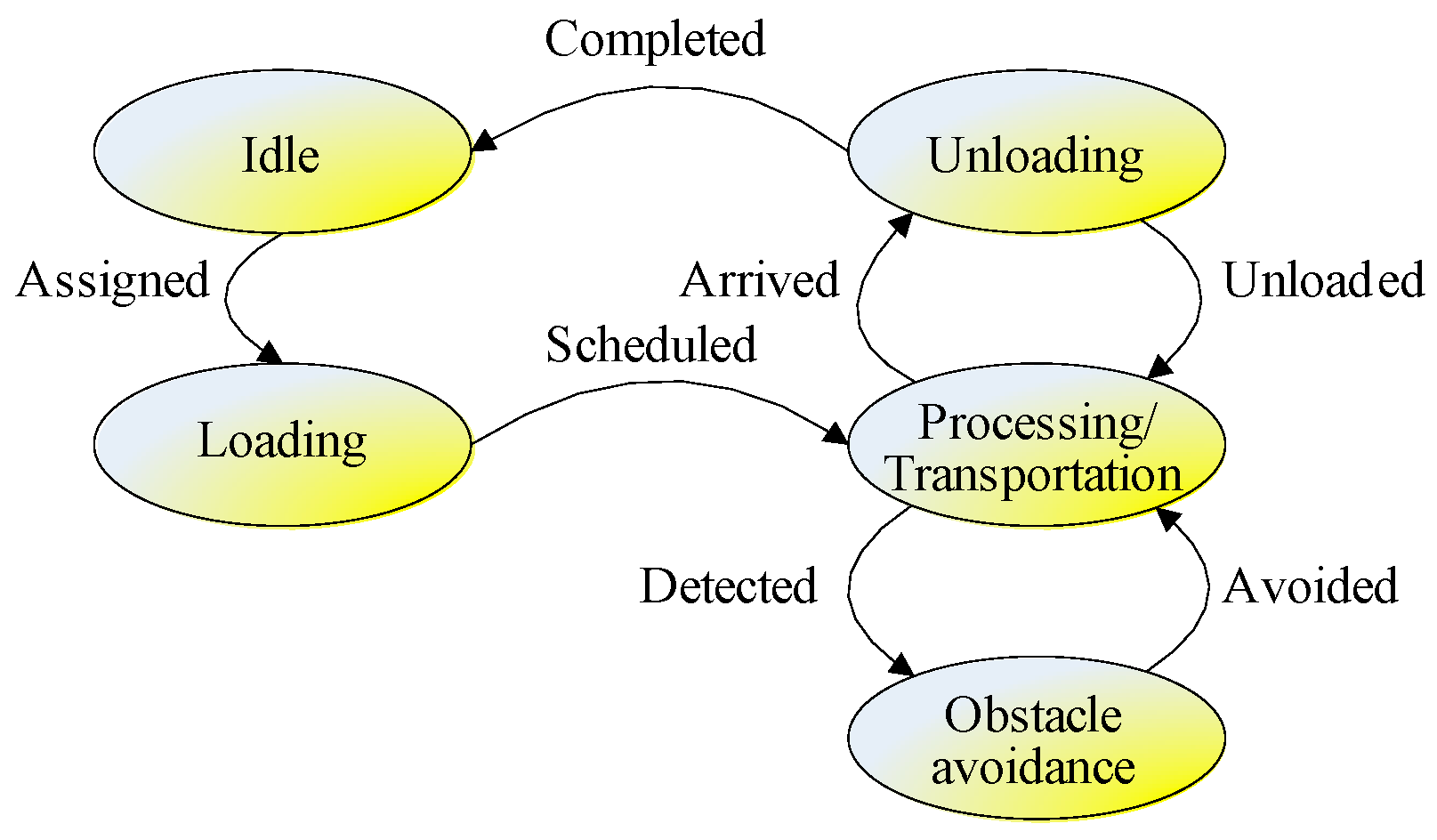
3.3. The State Transition Diagram for the POL
- Idle: This is an initial state where a machine/AGV is not assigned to any tasks. Only an idle machine/AGV can be assigned to a task;
- Loading: When a machine/AGV is assigned to a task, the idle machine/AGV is occupied and begins to load the cargo;
- Processing/Transportation: If a machine/AGV has loaded cargo for an assigned task, then it begins to process/transport the cargo;
- Obstacle avoidance: Whenever an obstacle is detected, the machine/AGV begins to adopt different strategies to avoid obstacles, including deceleration, acceleration, stop, and detour. When the obstacle is avoided, the machine/AGV will continue processing/transportation;
- Unloading: After the machine/AGV finishes processing/transportation, the machine/AGV will unload the cargo. If all cargo is unloaded and all tasks are completed, the machine/AGV will be in an idle state again and can be assigned to the next production task.
4. Problem Modeling
- All production tasks are assumed to be independent without considering their inter-relationships. There is no preference for the same production task on different machines or AGVs;
- All machines are assumed to be independent without considering their correlation with each other or their preferences for cargo;
- All AGVs are assumed to be independent without considering their correlation with each other or the differences in the loading of different cargo;
- The impact of the volume and shape of the cargo on processing and transportation time are not considered;
- The impact of working hours on the power changes in machines and AGVs are not considered. Sufficient power supply for machines and AGVs is assumed.
4.1. The Notations and Explanations
4.2. Task Planning in the VPL
4.3. AGV Optimization in the POL
5. APC-Based Edge Computing
5.1. Methodologies
5.2. Solution Steps of the APC
5.3. Algorithm Flow of the APC
| Algorithm 1: Solving the energy-efficient collision-free machine/AGV scheduling problem in the virtual planning layer | ||
| 1: | task state = new | |
| 2: | if AGV state = idle | |
| 3: | if assigned then task state = ready | |
| 4: | initialize the parameters of energy-efficient collision-free machine/AGV scheduling problem | |
| 5: | initialize the parameters of APC | |
| 6: | initialize the parameters of the solving system | |
| 7: | encode the APC individual by Equation (38) | |
| 8: | select fitness function by Equations (37) and (12) | |
| 9: | for ite = 1 to | |
| 10: | produce the random seeds by | |
| 11: | produce seeds from the previous fruits | |
| 12: | calculate fitness by Equations (37) and (12) | |
| 13: | choose the best solutions by | |
| 14: | choose the elite individual with the highest fitness | |
| 15: | choose a fruit through parthenogenesis | |
| 16: | produce fruits through social learning by | |
| 17: | end justification by | |
| 18: | end for | |
| 19: | output the optimal solution in the virtual planning layer | |
| 20: | if scheduled then task state = performing | |
| 21: | if interrupted then task state = waiting | |
| 22: | if completed then task state = exit | |
| Algorithm 2: Solving the energy-efficient collision-free machine/AGV scheduling problem in the physical optimization layer | ||
| 1: | if assigned then task state = optimization | |
| 2: | if machine/AGV state = idle | |
| 3: | input the best solution in the virtual planning layer | |
| 4: | initialize the parameters of energy-efficient collision-free machine/AGV scheduling problem | |
| 5: | initialize the parameters of APC | |
| 6: | initialize the parameters of the solving system | |
| 7: | encode the APC individual by Equation (39) | |
| 8: | select fitness function by Equations (37) and (28) | |
| 9: | for ite = 1 to | |
| 10: | produce the random seeds by | |
| 11: | produce seeds from the previous fruits | |
| 12: | calculate fitness by Equations (37) and (28) | |
| 13: | choose the best solutions by | |
| 14: | choose the elite individual with the highest fitness | |
| 15: | produce a fruit through parthenogenesis | |
| 16: | produce fruits through social learning by | |
| 17: | end justification by | |
| 18: | end for | |
| 19: | output the best solution in the physical optimization layer | |
| 20: | if scheduled then task state = performing | |
| 21: | if assigned then machine/AGV state = loading | |
| 22: | if scheduled then machine/AGV state = processing/transportation | |
| 23: | if detected then machine/AGV state = obstacle avoidance | |
| 24: | if detected then machine/AGV state = obstacle avoidance | |
| 25: | if avoided then machine/AGV state = processing/transportation | |
| 26: | if completed then machine/AGV state = idle | |
6. Benchmark Dataset and Tests
6.1. Benchmark Dataset
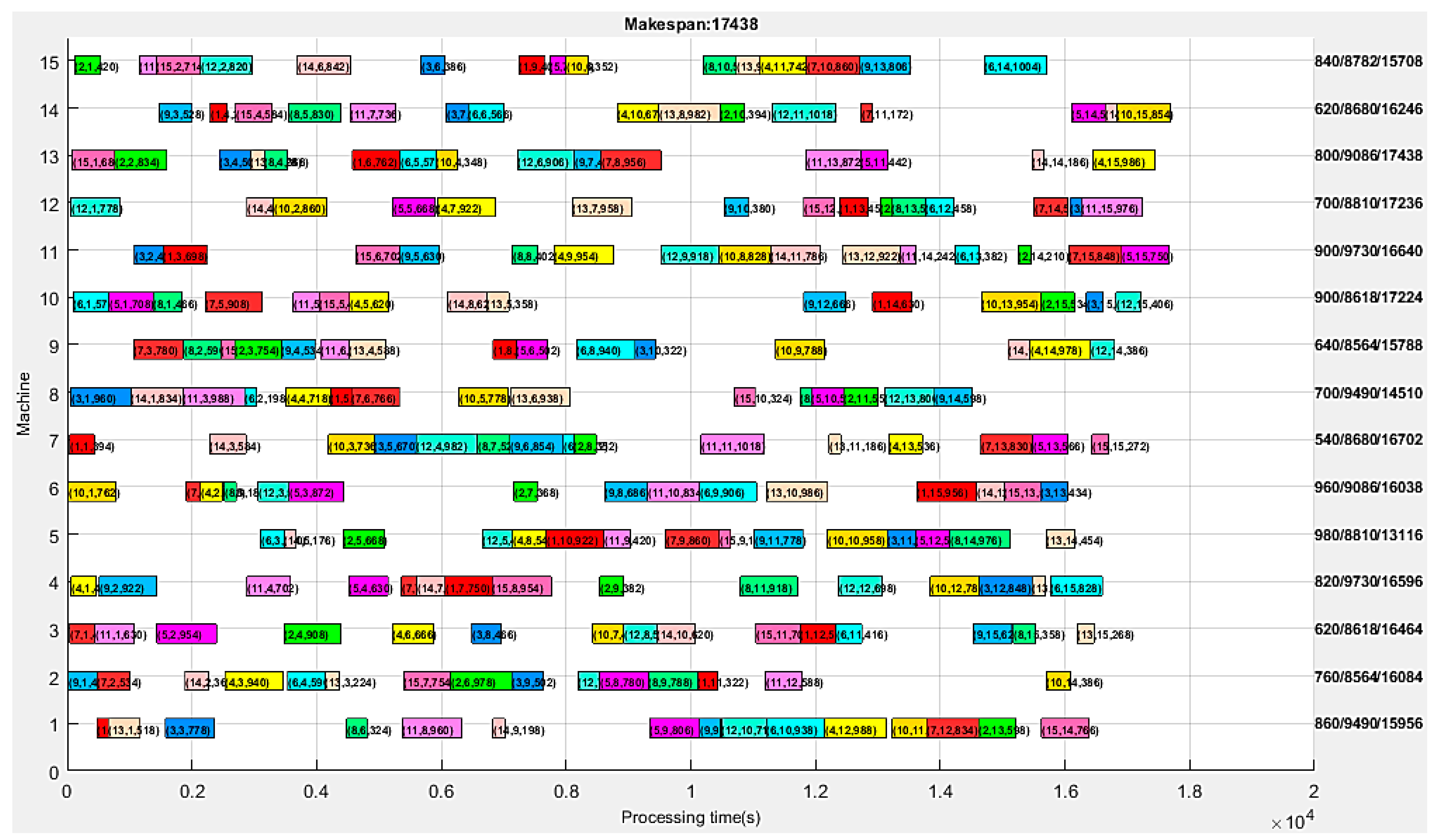
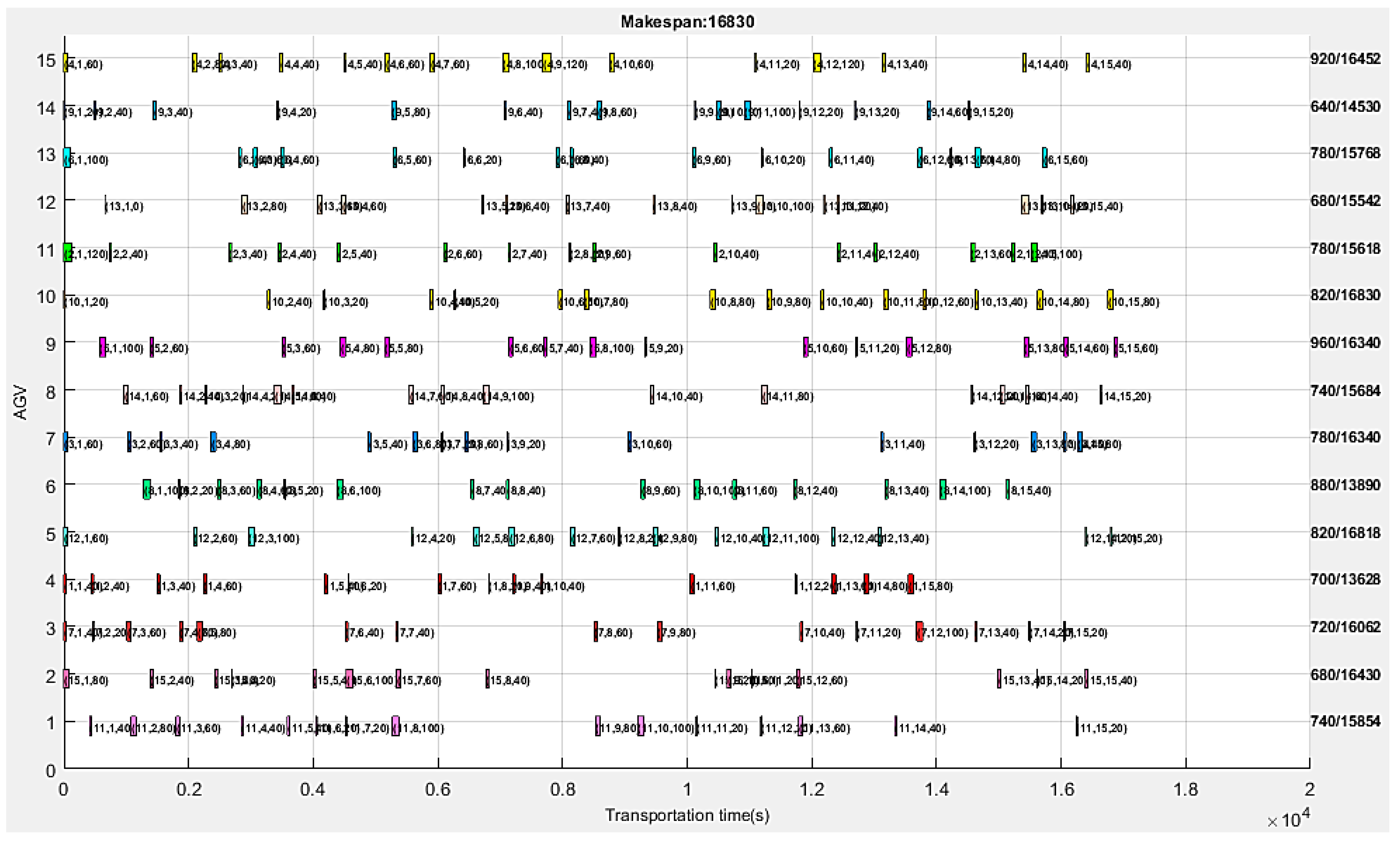
6.2. Numerical Experimental Results
6.3. Comparative Analysis
7. Conclusions
Author Contributions
Funding
Institutional Review Board Statement
Informed Consent Statement
Data Availability Statement
Acknowledgments
Conflicts of Interest
References
- Wang, Y.J.; Liu, X.Q.; Leng, J.Y.; Wang, J.J.; Meng, Q.N.; Zhou, M.J. Study on scheduling and path planning problems of multi-AGVs based on a heuristic algorithm in intelligent manufacturing workshop. Adv. Prod. Eng. Manag. 2022, 17, 505–513. [Google Scholar] [CrossRef]
- Chen, S.; Zhang, Q.; He, G.C.; Wu, Y.B. Multiple-AGV path planning method for two industrial links. Int. J. Pattern Recognit. Artif. Intell. 2022, 36, 2259029. [Google Scholar] [CrossRef]
- Lian, Y.; Yang, Q.; Xie, W.; Zhang, L. Cyber-physical system-based heuristic planning and scheduling method for multiple automatic guided vehicles in logistics systems. IEEE Trans. Ind. Inform. 2021, 17, 7882–7893. [Google Scholar] [CrossRef]
- Guo, Z.; Xia, Y.; Li, J.; Liu, J.; Xu, K. Hybrid optimization path planning method for AGV based on KGWO. Sensors 2024, 24, 5898. [Google Scholar] [CrossRef] [PubMed]
- Sanogo, K.; Benhafssa, A.M.; Sahnoun, M.; Bettayeb, B.; Abderrahim, M.; Bekrar, A. A multi-agent system simulation based approach for collision avoidance in integrated job-shop scheduling problem with transportation tasks. J. Manuf. Syst. 2023, 68, 209–226. [Google Scholar] [CrossRef]
- Goli, A.; Tirkolaee, E.B.; Aydin, N.S. Fuzzy integrated cell formation and production scheduling considering automated guided vehicles and human factors. IEEE Trans. Fuzzy Syst. 2021, 29, 3686–3695. [Google Scholar] [CrossRef]
- Cuan, Z.; Ding, D.W.; Wang, H.; Liu, Y.H.; Liu, Y.L. Simultaneous collision avoiding and target tracking for unmanned ground vehicle with velocity and heading rate constraints. Int. J. Control Autom. Syst. 2023, 21, 1222–1232. [Google Scholar] [CrossRef]
- Wang, J.; Li, S.; Li, B.; Zhao, C.; Cui, Y. An energy-efficient hierarchical algorithm of dynamic obstacle avoidance for unmanned surface vehicle. Int. J. Nav. Archit. Ocean. Eng. 2023, 15, 100528. [Google Scholar] [CrossRef]
- Cheng, W.; Meng, W. An efficient genetic algorithm for multi AGV scheduling problem about intelligent warehouse. Robot. Intell. Autom. 2023, 43, 382–393. [Google Scholar] [CrossRef]
- Luo, J.L.; Wan, Y.X.; Wu, W.M.; Li, Z.W. Optimal Petri-net controller for avoiding collisions in a class of automated guided vehicle systems. IEEE Trans. Intell. Transp. Syst. 2020, 21, 4526–4537. [Google Scholar] [CrossRef]
- Boufellouh, R.; Belkaid, F. Multi-objective optimization for energy-efficient flow shop scheduling problem with blocking and collision-free transportation constraints. Appl. Soft Comput. 2023, 148, 110884. [Google Scholar] [CrossRef]
- Deng, S.G.; Zhao, H.L.; Fang, W.J.; Yin, J.W.; Dustdar, S.; Zomaya, A.Y. Edge intelligence: The confluence of edge computing and artificial intelligence. IEEE Internet Things J. 2020, 7, 7457–7469. [Google Scholar] [CrossRef]
- Wang, J.; Li, Y.; Zhang, Z.; Wu, Z.; Wu, L.; Jia, S.; Peng, T. Dynamic integrated scheduling of production equipment and automated guided vehicles in a flexible job shop based on deep reinforcement learning. Processes 2024, 12, 2423. [Google Scholar] [CrossRef]
- Chen, Y.; Chen, M.; Yu, F.; Lin, H.; Yi, W. An improved ant colony algorithm with deep reinforcement learning for the robust multiobjective AGV routing problem in assembly workshops. Appl. Sci. 2024, 14, 7135. [Google Scholar] [CrossRef]
- Zhong, Z.; Guo, Y.; Zhang, J.; Yang, S. Energy-aware integrated scheduling for container terminals with conflict-free AGVs. J. Syst. Sci. Syst. Eng. 2023, 32, 413–443. [Google Scholar] [CrossRef]
- Zhang, L.; Kan, H.; Wang, Y. Privacy-Preserving AGV collision-resistance at the edge using location-based encryption. IEEE Trans. Serv. Comput. 2023, 16, 2868–2878. [Google Scholar] [CrossRef]
- Cai, Y.; Liu, H.; Li, M.; Ren, F. A method of dual-AGV-ganged path planning based on the genetic algorithm. Appl. Sci. 2024, 14, 7482. [Google Scholar] [CrossRef]
- Cai, Z.; Jiang, S.; Dong, J.; Tang, S. An artificial plant community algorithm for the accurate range-free positioning of wireless sensor networks. Sensors 2023, 23, 2804. [Google Scholar] [CrossRef] [PubMed]
- Cai, Z.; Ma, Z.; Zuo, Z.; Xiang, Y.; Wang, M. An image edge detection algorithm based on an artificial plant community. Appl. Sci. 2023, 13, 4159. [Google Scholar] [CrossRef]
- Sebem, R.; Leal, A.B.; Bertol, D.W.; da Silva, M.F.; Teles, M.G. Architecture for scalable and distributed control of connected and automated vehicles with reconfigurable path planning. IEEE Trans. Autom. Sci. Eng. 2024, 21, 5583–5598. [Google Scholar] [CrossRef]
- Xu, B.; Jie, D.; Li, J.; Zhou, Y.; Wang, H.; Fan, H. A hybrid dynamic method for conflict-free integrated schedule optimization in u-shaped automated container terminals. J. Mar. Sci. Eng. 2022, 10, 1187. [Google Scholar] [CrossRef]
- Liang, C.; Zhang, Y.; Dong, L. A three stage optimal scheduling algorithm for AGV route planning considering collision avoidance under speed control strategy. Mathematics 2023, 11, 138. [Google Scholar] [CrossRef]
- Li, C.; Zhang, L.; Zhang, L. A route and speed optimization model to find conflict-free routes for automated guided vehicles in large warehouses based on quick response code technology. Adv. Eng. Inform. 2022, 52, 101604. [Google Scholar] [CrossRef]
- Malopolski, W.; Zajac, J. AGVs collision and deadlock handling based on structural online control policy: A case study in a square topology. Appl. Sci. 2021, 11, 6494. [Google Scholar] [CrossRef]
- Zhou, B.; Lei, Y. The pickup and delivery hybrid-operations of AGV conflict-free scheduling problem with time constraint among multi-FMCs. Neural Comput. Appl. 2023, 35, 23125–23151. [Google Scholar] [CrossRef]
- Sun, J.; Xu, Z.; Yan, Z.; Liu, L.; Zhang, Y. An approach to integrated scheduling of flexible job-shop considering conflict-free routing problems. Sensors 2023, 23, 4526. [Google Scholar] [CrossRef] [PubMed]
- Li, P.; Yang, L. Conflict-free and energy-efficient path planning for multi-robots based on priority free ant colony optimization. Math. Biosci. Eng. 2023, 20, 3528–3565. [Google Scholar] [CrossRef] [PubMed]
- Iveta, K.; Jaroslava, K.; Dominik, B.; Dominika, K. Implementation of automated guided vehicles for the automation of selected processes and elimination of collisions between handling equipment and humans in the warehouse. Sensors 2024, 24, 1029. [Google Scholar] [CrossRef]
- Lin, S.; Liu, A.; Wang, J.; Kong, X. An intelligence-based hybrid PSO-SA for mobile robot path planning in warehouse. J. Comput. Sci. 2023, 67, 101938. [Google Scholar] [CrossRef]
- Lin, S.; Liu, A.; Wang, J.; Kong, X. An improved fault-tolerant cultural-PSO with probability for multi-AGV path planning. Expert Syst. Appl. 2024, 237, 121510. [Google Scholar] [CrossRef]
- Luo, L.; Zhao, N.; Zhu, Y.; Sun, Y. A* guiding DQN algorithm for automated guided vehicle pathfinding problem of robotic mobile fulfillment systems. Comput. Ind. Eng. 2023, 178, 109112. [Google Scholar] [CrossRef]
- Mugarza, I.; Carlos, M.J. A coloured petri net- and D* lite-based traffic controller for automated guided vehicles. Electronics 2021, 10, 2235. [Google Scholar] [CrossRef]
- Adamo, T.; Ghiani, G.; Guerriero, E. Recovering feasibility in real-time conflict-free vehicle routing. Comput. Ind. Eng. 2023, 183, 109437. [Google Scholar] [CrossRef]
- Zhou, Y.; Huang, N. Airport AGV path optimization model based on ant colony algorithm to optimize Dijkstra algorithm in urban systems. Sustain. Comput. Inform. Syst. 2022, 35, 100716. [Google Scholar] [CrossRef]
- Hu, L.; Zhao, X.; Liu, W.; Cai, W.; Xu, K.; Zhang, Z. Energy benchmark for energy-efficient path planning of the automated guided vehicle. Sci. Total Environ. 2023, 857, 159613. [Google Scholar] [CrossRef] [PubMed]
- He, L.; Chiong, R.; Li, W. Energy-efficient open-shop scheduling with multiple automated guided vehicles and deteriorating jobs. J. Ind. Inf. Integr. 2022, 30, 100387. [Google Scholar] [CrossRef]
- Nabovati, H.; Haleh, H.; Vahdani, B. Multi-objective invasive weeds optimisation algorithm for solving simultaneous scheduling of machines and multi-mode automated guided vehicles. Eur. J. Ind. Eng. 2020, 14, 165–188. [Google Scholar] [CrossRef]
- Zhang, L.; Yan, Y.; Hu, Y. Deep reinforcement learning for dynamic scheduling of energy-efficient automated guided vehicles. J. Intell. Manuf. 2024, 35, 3875–3888. [Google Scholar] [CrossRef]
- Cai, Z.; Li, G.Z.; Zhang, J.M.; Xiong, S.S. Using an artificial Physarum polycephalum colony for threshold image segmentation. Appl. Sci. 2023, 13, 11976. [Google Scholar] [CrossRef]
- Cai, Z.; Feng, Y.; Yang, S.; Yang, J. A state transition diagram and an artificial physarum polycephalum colony algorithm for the flexible job shop scheduling problem with transportation constraints. Processes 2023, 11, 2646. [Google Scholar] [CrossRef]
- Arash, A.; Erfan, B.T.; Vladimir, S.; Gerhard-Wilhelm, W. A parallel heuristic for hybrid job shop scheduling problem considering conflict-free AGV routing. Swarm Evol. Comput. 2023, 79, 101312. [Google Scholar]
- Aizat, M.; Qistina, N.; Rahiman, W. A comprehensive review of recent advances in automated guided vehicle technologies: Dynamic obstacle avoidance in complex environment toward autonomous capability. IEEE Trans. Instrum. Meas. 2024, 73, 8500125. [Google Scholar] [CrossRef]


| The Virtual Planning Layer | The Physical Optimization Layer | |
|---|---|---|
| Level | Top layer | Bottom layer |
| Definition | Virtual entity | Physical entity |
| Role | Edge servers | Edge AGVs |
| Attribute | Fixed | Mobile |
| Function | Pre-arrange | Real time |
| Architecture | Integrated | Distributed |
| Computational ability | Server level | Embedded platforms |
| Storage capacity | Server level | Embedded platforms |
| Notations | Explanation |
|---|---|
| A production task | |
| Time | |
| The objective function | |
| An arc set | |
| A set of machines | |
| A set of edges | |
| A set of cargo | |
| A set of AGVs | |
| The node number | |
| The AGV number | |
| The cargo number | |
| Total number of tasks | |
| Total number of machines | |
| Total number of cargoes | |
| Total number of AGVs | |
| An edge between the nodes and | |
| The distance between the two nodes | |
| The total load of all cargo in a task | |
| The load of cargo | |
| The load of AGV | |
| The maximum load capacity of AGV | |
| The load factor of AGV | |
| The maximum load factor of AGV | |
| The minimum load factor of AGV | |
| The route of AGV | |
| The total distance of route | |
| The route balance index of AGV | |
| A selection bit of AGV , . =1 if cargo is on AGV ; otherwise, =0. | |
| A selection bit of route , . =1 if is on route ; otherwise, =0. | |
| The start node of route | |
| The end node of route | |
| The driving speed of AGV | |
| The maximum driving speed of AGV | |
| The battery capacity of AGV | |
| The total energy consumption of a task | |
| The total energy consumption of AGV | |
| The total energy consumption of machine | |
| The energy consumption of AGV on edge | |
| The energy consumption of cargo on node | |
| The driving power of AGV | |
| The stop power of AGV | |
| The turning power of AGV | |
| The acceleration power of AGV | |
| The processing power when cargo is on node | |
| The driving force of AGV | |
| The stop force of AGV | |
| The turning force of AGV | |
| The acceleration force of AGV | |
| The unit time window of AGV on edge | |
| The total time cost (makespan) of a task | |
| The longest travel time of AGVs | |
| The total time cost of machine | |
| The total collision time on all nodes | |
| The time when AGV enters node | |
| The time when AGV leaves the current node | |
| The processing time when cargo is on node | |
| The collision time on node | |
| The stop time of AGV on edge | |
| The turning time of AGV on edge | |
| The acceleration time of AGV on edge |
| Machines | |||||||||||||||
|---|---|---|---|---|---|---|---|---|---|---|---|---|---|---|---|
| 0 | 20 | 40 | 60 | 80 | 20 | 40 | 60 | 80 | 100 | 40 | 60 | 80 | 100 | 120 | |
| 20 | 0 | 20 | 40 | 60 | 40 | 20 | 40 | 60 | 80 | 60 | 40 | 60 | 80 | 100 | |
| 40 | 20 | 0 | 20 | 40 | 60 | 40 | 20 | 40 | 60 | 80 | 60 | 40 | 60 | 80 | |
| 60 | 40 | 20 | 0 | 20 | 80 | 60 | 40 | 20 | 40 | 100 | 80 | 60 | 40 | 60 | |
| 80 | 60 | 40 | 20 | 0 | 100 | 80 | 60 | 40 | 20 | 120 | 100 | 80 | 60 | 40 | |
| 20 | 40 | 60 | 80 | 100 | 0 | 20 | 40 | 60 | 80 | 20 | 40 | 60 | 80 | 100 | |
| 40 | 20 | 40 | 60 | 80 | 20 | 0 | 20 | 40 | 60 | 40 | 20 | 40 | 60 | 80 | |
| 60 | 40 | 20 | 40 | 60 | 40 | 20 | 0 | 20 | 40 | 60 | 40 | 20 | 40 | 60 | |
| 80 | 60 | 40 | 20 | 40 | 60 | 40 | 20 | 0 | 20 | 80 | 60 | 40 | 20 | 40 | |
| 100 | 80 | 60 | 40 | 20 | 80 | 60 | 40 | 20 | 0 | 100 | 80 | 60 | 40 | 20 | |
| 40 | 60 | 80 | 100 | 120 | 20 | 40 | 60 | 80 | 100 | 0 | 20 | 40 | 60 | 80 | |
| 60 | 40 | 60 | 80 | 100 | 40 | 20 | 40 | 60 | 80 | 20 | 0 | 20 | 40 | 60 | |
| 80 | 60 | 40 | 60 | 80 | 60 | 40 | 20 | 40 | 60 | 40 | 20 | 0 | 20 | 40 | |
| 100 | 80 | 60 | 40 | 60 | 80 | 60 | 40 | 20 | 40 | 60 | 40 | 20 | 0 | 20 | |
| 120 | 100 | 80 | 60 | 40 | 100 | 80 | 60 | 40 | 20 | 80 | 60 | 40 | 20 | 0 |
| Cargo | |||||||||||||||
|---|---|---|---|---|---|---|---|---|---|---|---|---|---|---|---|
| 180 | 598 | 778 | 988 | 806 | 938 | 834 | 324 | 332 | 552 | 960 | 718 | 518 | 198 | 766 | |
| 322 | 978 | 502 | 940 | 780 | 596 | 534 | 788 | 456 | 386 | 588 | 348 | 224 | 368 | 754 | |
| 570 | 908 | 466 | 666 | 954 | 416 | 406 | 358 | 622 | 492 | 630 | 534 | 268 | 620 | 708 | |
| 750 | 382 | 848 | 402 | 630 | 828 | 242 | 918 | 922 | 786 | 702 | 698 | 210 | 458 | 954 | |
| 922 | 668 | 458 | 540 | 548 | 380 | 860 | 976 | 778 | 958 | 420 | 490 | 454 | 176 | 182 | |
| 956 | 368 | 434 | 348 | 872 | 906 | 228 | 186 | 686 | 762 | 834 | 500 | 986 | 442 | 578 | |
| 394 | 352 | 670 | 536 | 566 | 172 | 830 | 528 | 854 | 736 | 1018 | 982 | 186 | 584 | 272 | |
| 332 | 552 | 960 | 718 | 518 | 198 | 766 | 180 | 598 | 778 | 988 | 806 | 938 | 834 | 324 | |
| 368 | 754 | 322 | 978 | 502 | 940 | 780 | 596 | 534 | 788 | 456 | 386 | 588 | 348 | 224 | |
| 630 | 534 | 268 | 620 | 708 | 570 | 908 | 466 | 666 | 954 | 416 | 406 | 358 | 622 | 492 | |
| 698 | 210 | 458 | 954 | 750 | 382 | 848 | 402 | 630 | 828 | 242 | 918 | 922 | 786 | 702 | |
| 454 | 176 | 182 | 922 | 668 | 458 | 540 | 548 | 380 | 860 | 976 | 778 | 958 | 420 | 490 | |
| 762 | 834 | 500 | 986 | 442 | 578 | 956 | 368 | 434 | 348 | 872 | 906 | 228 | 186 | 686 | |
| 272 | 394 | 352 | 670 | 536 | 566 | 172 | 830 | 528 | 854 | 736 | 1018 | 982 | 186 | 584 | |
| 406 | 420 | 386 | 742 | 254 | 1004 | 860 | 526 | 806 | 352 | 270 | 820 | 380 | 842 | 714 |
| Rate | 1 | 2 | 3 | 4 | 5 |
|---|---|---|---|---|---|
| Speed (m/s) | 0.4 | 0.5 | 0.67 | 1.0 | 2.0 |
| Power consumption (W) | 60.4 | 82.8 | 119.2 | 191.2 | 405.8 |
| The load factor, | 1.0 | 1.0 | 1.0 | 0.9 | 0.8 |
| 1.22 | 1.22 | 1.03 | 1.03 | 1.14 | 1.14 | 1.01 | 1.01 | 1.12 | 1.12 | 1.21 | 1.21 | 1.10 | 1.10 | 0.90 |
| Process | 1 | 2 | 3 | 4 | 5 | 6 | 7 | 8 | 9 | 10 | 11 | 12 | 13 | 14 | 15 | |
|---|---|---|---|---|---|---|---|---|---|---|---|---|---|---|---|---|
| Machine | ||||||||||||||||
| 15 | (2, 1, 420) | (11, 2, 270) | (15, 2, 714) | (12, 2, 820) | (14, 6, 842) | (3, 6, 386) | (1, 9, 406) | (5, 7, 254) | (10, 6, 352) | (8, 10, 526) | (13, 9, 380) | (4, 11, 742) | (7, 10, 860) | (9, 13, 806) | (6, 14, 1004) | |
| 14 | (9, 3, 528) | (1, 4, 272) | (15, 4, 584) | (8, 5, 830) | (11, 7, 736) | (3, 7, 352) | (6, 6, 566) | (4, 10, 670) | (13, 8, 982) | (2, 10, 394) | (12, 11, 1018) | (7, 11, 172) | (5, 14, 536) | (14, 15, 186) | (10, 15, 854) | |
| 13 | (15, 1, 686) | (2, 2, 834) | (3, 4, 500) | (13, 2, 228) | (8, 4, 368) | (1, 6, 762) | (6, 5, 578) | (10, 4, 348) | (12, 6, 906) | (9, 7, 434) | (7, 8, 956) | (11, 13, 872) | (5, 11, 442) | (14, 14, 186) | (4, 15, 986) | |
| 12 | (12, 1, 778) | (14, 4, 420) | (10, 2, 860) | (5, 5, 668) | (4, 7, 922) | (13, 7, 958) | (9, 10, 380) | (15, 12, 490) | (1, 13, 454) | (2, 12, 176) | (8, 13, 548) | (6, 12, 458) | (7, 14, 540) | (3, 14, 182) | (11, 15, 976) | |
| 11 | (3, 2, 458) | (1, 3, 698) | (15, 6, 702) | (9, 5, 630) | (8, 8, 402) | (4, 9, 954) | (12, 9, 918) | (10, 8, 828) | (14, 11, 786) | (13, 12, 922) | (11, 14, 242) | (6, 13, 382) | (2, 14, 210) | (7, 15, 848) | (5, 15, 750) | |
| 10 | (6, 1, 570) | (5, 1, 708) | (8, 1, 466) | (7, 5, 908) | (11, 5, 416) | (15, 5, 492) | (4, 5, 620) | (14, 8, 622) | (13, 5, 358) | (9, 12, 666) | (1, 14, 630) | (10, 13, 954) | (2, 15, 534) | (3, 15, 268) | (12, 15, 406) | |
| 9 | (7, 3, 780) | (8, 2, 596) | (15, 3, 224) | (2, 3, 754) | (9, 4, 534) | (11, 6, 456) | (13, 4, 588) | (1, 8, 368) | (5, 6, 502) | (6, 8, 940) | (3, 10, 322) | (10, 9, 788) | (14, 13, 348) | (4, 14, 978) | (12, 14, 386) | |
| 8 | (3, 1, 960) | (14, 1, 834) | (11, 3, 988) | (6, 2, 198) | (4, 4, 718) | (1, 5, 332) | (7, 6, 766) | (10, 5, 778) | (13, 6, 938) | (15, 10, 324) | (8, 12, 180) | (5, 10, 518) | (2, 11, 552) | (12, 13, 806) | (9, 14, 598) | |
| 7 | (1, 1, 394) | (14, 3, 584) | (10, 3, 736) | (3, 5, 670) | (12, 4, 982) | (8, 7, 528) | (9, 6, 854) | (6, 7, 172) | (2, 8, 352) | (11, 11, 1018) | (13, 11, 186) | (4, 13, 536) | (7, 13, 830) | (5, 13, 566) | (15, 15, 272) | |
| 6 | (10, 1, 762) | (7, 4, 228) | (4, 2, 348) | (8, 3, 186) | (12, 3, 500) | (5, 3, 872) | (2, 7, 368) | (9, 8, 686) | (11, 10, 834) | (6, 9, 906) | (13, 10, 986) | (1, 15, 956) | (14, 12, 442) | (15, 13, 578) | (3, 13, 434) | |
| 5 | (6, 3, 380) | (14, 5, 176) | (2, 5, 668) | (12, 5, 490) | (4, 8, 540) | (1, 10, 922) | (11, 9, 420) | (7, 9, 860) | (15, 9, 182) | (9, 11, 778) | (10, 10, 958) | (3, 11, 458) | (5, 12, 548) | (8, 14, 976) | (13, 14, 454) | |
| 4 | (4, 1, 402) | (9, 2, 922) | (11, 4, 702) | (5, 4, 630) | (7, 7, 242) | (14, 7, 458) | (1, 7, 750) | (15, 8, 954) | (2, 9, 382) | (8, 11, 918) | (12, 12, 698) | (10, 12, 786) | (3, 12, 848) | (13, 13, 210) | (6, 15, 828) | |
| 3 | (7, 1, 406) | (11, 1, 630) | (5, 2, 954) | (2, 4, 908) | (4, 6, 666) | (3, 8, 466) | (10, 7, 492) | (12, 8, 534) | (14, 10, 620) | (15, 11, 708) | (1, 12, 570) | (6, 11, 416) | (9, 15, 622) | (8, 15, 358) | (13, 15, 268) | |
| 2 | (9, 1, 456) | (7, 2, 534) | (14, 2, 368) | (4, 3, 940) | (6, 4, 596) | (13, 3, 224) | (15, 7, 754) | (2, 6, 978) | (3, 9, 502) | (12, 7, 348) | (5, 8, 780) | (8, 9, 788) | (1, 11, 322) | (11, 12, 588) | (10, 14, 386) | |
| 1 | (1, 2, 180) | (13, 1, 518) | (3, 3, 778) | (8, 6, 324) | (11, 8, 960) | (14, 9, 198) | (5, 9, 806) | (9, 9, 332) | (12, 10, 718) | (6, 10, 938) | (4, 12, 988) | (10, 11, 552) | (7, 12, 834) | (2, 13, 598) | (15, 14, 766) | |
| Transportation | 1 | 2 | 3 | 4 | 5 | 6 | 7 | 8 | 9 | 10 | 11 | 12 | 13 | 14 | 15 | |
|---|---|---|---|---|---|---|---|---|---|---|---|---|---|---|---|---|
| AGV | ||||||||||||||||
| 15 | (4, 1, 60) | (4, 2, 80) | (4, 3, 40) | (4, 4, 40) | (4, 5, 40) | (4, 6, 60) | (4, 7, 60) | (4, 8, 100) | (4, 9, 120) | (4, 10, 60) | (4, 11, 20) | (4, 12, 120) | (4, 13, 40) | (4, 14, 40) | (4, 15, 40) | |
| 14 | (9, 1, 20) | (9, 2, 40) | (9, 3, 40) | (9, 4, 20) | (9, 5, 80) | (9, 6, 40) | (9, 7, 40) | (9, 8, 60) | (9, 9, 20) | (9, 10, 60) | (9, 11, 100) | (9, 12, 20) | (9, 13, 20) | (9, 14, 60) | (9, 15, 20) | |
| 13 | (6, 1, 100) | (6, 2, 40) | (6, 3, 60) | (6, 4, 60) | (6, 5, 60) | (6, 6, 20) | (6, 7, 60) | (6, 8, 40) | (6, 9, 60) | (6, 10, 20) | (6, 11, 40) | (6, 12, 60) | (6, 13, 20) | (6, 14, 80) | (6, 15, 60) | |
| 12 | (13, 1, 0) | (13, 2, 80) | (13, 3, 60) | (13, 4, 60) | (13, 5, 20) | (13, 6, 40) | (13, 7, 40) | (13, 8, 40) | (13, 9, 20) | (13, 10, 100) | (13, 11, 20) | (13, 12, 40) | (13, 13, 100) | (13, 14, 20) | (13, 15, 40) | |
| 11 | (2, 1, 120) | (2, 2, 40) | (2, 3, 40) | (2, 4, 40) | (2, 5, 40) | (2, 6, 60) | (2, 7, 40) | (2, 8, 20) | (2, 9, 60) | (2, 10, 40) | (2, 11, 40) | (2, 12, 40) | (2, 13, 60) | (2, 14, 40) | (2, 15, 100) | |
| 10 | (10, 1, 20) | (10, 2, 40) | (10, 3, 20) | (10, 4, 40) | (10, 5, 20) | (10, 6, 60) | (10, 7, 80) | (10, 8, 80) | (10, 9, 80) | (10, 10, 40) | (10, 11, 80) | (10, 12, 60) | (10, 13, 40) | (10, 14, 80) | (10, 15, 80) | |
| 9 | (5, 1, 100) | (5, 2, 60) | (5, 3, 60) | (5, 4, 80) | (5, 5, 80) | (5, 6, 60) | (5, 7, 40) | (5, 8, 100) | (5, 9, 20) | (5, 10, 60) | (5, 11, 20) | (5, 12, 80) | (5, 13, 80) | (5, 14, 60) | (5, 15, 60) | |
| 8 | (14, 1, 60) | (14, 2, 40) | (14, 3, 20) | (14, 4, 20) | (14, 5, 100) | (14, 6, 40) | (14, 7, 60) | (14, 8, 40) | (14, 9, 100) | (14, 10, 40) | (14, 11, 80) | (14, 12, 20) | (14, 13, 60) | (14, 14, 40) | (14, 15, 20) | |
| 7 | (3, 1, 60) | (3, 2, 60) | (3, 3, 40) | (3, 4, 80) | (3, 5, 40) | (3, 6, 80) | (3, 7, 20) | (3, 8, 60) | (3, 9, 20) | (3, 10, 60) | (3, 11, 40) | (3, 12, 20) | (3, 13, 80) | (3, 14, 40) | (3, 15, 80) | |
| 6 | (8, 1, 100) | (8, 2, 20) | (8, 3, 60) | (8, 4, 60) | (8, 5, 20) | (8, 6, 100) | (8, 7, 40) | (8, 8, 40) | (8, 9, 60) | (8, 10, 100) | (8, 11, 60) | (8, 12, 40) | (8, 13, 40) | (8, 14, 100) | (8, 15, 40) | |
| 5 | (12, 1, 60) | (12, 2, 60) | (12, 3, 100) | (12, 4, 20) | (12, 5, 80) | (12, 6, 80) | (12, 7, 60) | (12, 8, 20) | (12, 9, 80) | (12, 10, 40) | (12, 11, 100) | (12, 12, 40) | (12, 13, 40) | (12, 14, 20) | (12, 15, 20) | |
| 4 | (1, 1, 40) | (1, 2, 40) | (1, 3, 40) | (1, 4, 60) | (1, 5, 40) | (1, 6, 20) | (1, 7, 60) | (1, 8, 20) | (1, 9, 40) | (1, 10, 40) | (1, 11, 60) | (1, 12, 20) | (1, 13, 60) | (1, 14, 80) | (1, 15, 80) | |
| 3 | (7, 1, 40) | (7, 2, 20) | (7, 3, 60) | (7, 4, 60) | (7, 5, 80) | (7, 6, 40) | (7, 7, 40) | (7, 8, 60) | (7, 9, 80) | (7, 10, 40) | (7, 11, 20) | (7, 12, 100) | (7, 13, 40) | (7, 14, 20) | (7, 15, 20) | |
| 2 | (15, 1, 80) | (15, 2, 40) | (15, 3, 40) | (15, 4, 20) | (15, 5, 40) | (15, 6, 100) | (15, 7, 60) | (15, 8, 40) | (15, 9, 20) | (15, 10, 60) | (15, 11, 20) | (15, 12, 60) | (15, 13, 40) | (15, 14, 20) | (15, 15, 40) | |
| 1 | (11, 1, 40) | (11, 2, 80) | (11, 3, 60) | (11, 4, 40) | (11, 5, 40) | (11, 6, 20) | (11, 7, 20) | (11, 8, 100) | (11, 9, 80) | (11, 10, 100) | (11, 11, 20) | (11, 12, 20) | (11, 13, 60) | (11, 14, 40) | (11, 15, 20) | |
| Indicator | Solutions | ||
|---|---|---|---|
| Minimum | Average | Maximum | |
| The makespan of a task (s) | 17,438 | 18,455.5 | 20,016 |
| The total energy consumption of a task (kWh) | 41.952 | 41.975 | 41.989 |
| The total collision time on all nodes (s) | 0.00 | 0.00 | 0.00 |
| The route balance index of AGV (m) | 280 | 320 | 360 |
| The longest travel time of AGV (s) | 920 | 965 | 1000 |
| Total processing energy (kWh) | 41.334 | 41.334 | 41.334 |
| Total AGV energy consumption (kWh) | 0.618 | 0.642 | 0.655 |
| Total traveled distance (m) | 11,640 | 12,085 | 12,340 |
| The lowest AGV speed (m/s) | 1.0 | 1.0 | 1.0 |
| Method | Number of Machines | Mean | ||||||||
|---|---|---|---|---|---|---|---|---|---|---|
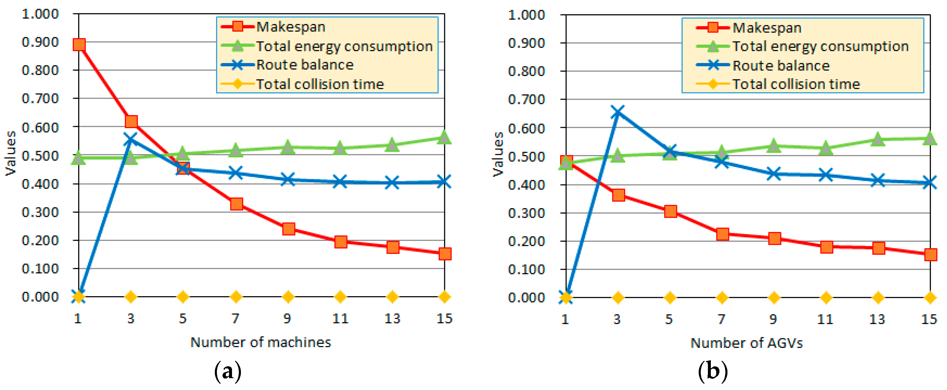
| APC | Makespan | 0.893 | 0.622 | 0.455 | 0.329 | 0.241 | 0.197 | 0.176 | 0.154 | 0.383 |
| Total energy consumption | 0.489 | 0.491 | 0.506 | 0.516 | 0.528 | 0.523 | 0.537 | 0.563 | 0.519 | |
| Total collision time | 0.000 | 0.000 | 0.000 | 0.000 | 0.000 | 0.000 | 0.000 | 0.000 | 0.000 | |
| Route balance index | 0.000 | 0.557 | 0.453 | 0.438 | 0.415 | 0.405 | 0.402 | 0.407 | 0.385 | |
| Solution time (s) | 412 | 405 | 428 | 433 | 447 | 446 | 459 | 461 | 436.375 | |
| GA | Makespan | 0.922 | 0.639 | 0.504 | 0.353 | 0.240 | 0.245 | 0.212 | 0.172 | 0.411 |
| Total energy consumption | 0.494 | 0.503 | 0.519 | 0.532 | 0.536 | 0.521 | 0.547 | 0.575 | 0.528 | |
| Total collision time | 0.000 | 0.000 | 0.000 | 0.000 | 0.000 | 0.000 | 0.000 | 0.000 | 0.000 | |
| Route balance index | 0.000 | 0.568 | 0.457 | 0.447 | 0.412 | 0.421 | 0.409 | 0.413 | 0.391 | |
| Solution time (s) | 401 | 396 | 438 | 436 | 443 | 454 | 450 | 459 | 434.625 | |
| ACO | Makespan | 0.928 | 0.657 | 0.472 | 0.366 | 0.260 | 0.253 | 0.209 | 0.166 | 0.414 |
| Total energy consumption | 0.498 | 0.507 | 0.522 | 0.539 | 0.541 | 0.546 | 0.544 | 0.568 | 0.533 | |
| Total collision time | 0.000 | 0.000 | 0.000 | 0.000 | 0.000 | 0.000 | 0.000 | 0.000 | 0.000 | |
| Route balance index | 0.000 | 0.563 | 0.466 | 0.434 | 0.426 | 0.418 | 0.411 | 0.422 | 0.393 | |
| Solution time (s) | 396 | 414 | 413 | 431 | 439 | 422 | 445 | 475 | 429.375 | |
| PSO | Makespan | 0.934 | 0.660 | 0.491 | 0.372 | 0.274 | 0.228 | 0.223 | 0.174 | 0.420 |
| Total energy consumption | 0.505 | 0.496 | 0.511 | 0.530 | 0.534 | 0.539 | 0.552 | 0.580 | 0.531 | |
| Total collision time | 0.000 | 0.000 | 0.000 | 0.000 | 0.000 | 0.000 | 0.000 | 0.000 | 0.000 | |
| Route balance index | 0.000 | 0.549 | 0.475 | 0.460 | 0.423 | 0.412 | 0.415 | 0.420 | 0.394 | |
| Solution time (s) | 419 | 398 | 411 | 425 | 442 | 453 | 447 | 472 | 433.375 | |
| DQN | Makespan | 0.916 | 0.620 | 0.458 | 0.331 | 0.256 | 0.195 | 0.189 | 0.160 | 0.391 |
| Total energy consumption | 0.493 | 0.518 | 0.497 | 0.514 | 0.529 | 0.532 | 0.535 | 0.564 | 0.523 | |
| Total collision time | 0.000 | 0.000 | 0.000 | 0.000 | 0.000 | 0.000 | 0.000 | 0.000 | 0.000 | |
| Route balance index | 0.000 | 0.559 | 0.454 | 0.449 | 0.418 | 0.406 | 0.405 | 0.407 | 0.387 | |
| Solution time (s) | 1845 | 1967 | 2084 | 2008 | 2016 | 2120 | 2171 | 2163 | 2046.75 | |
| Method | Number of AGVs | Mean | ||||||||
|---|---|---|---|---|---|---|---|---|---|---|
| APC | Makespan | 0.481 | 0.364 | 0.307 | 0.226 | 0.212 | 0.179 | 0.176 | 0.154 | 0.262 |
| Total energy consumption | 0.475 | 0.502 | 0.508 | 0.514 | 0.537 | 0.530 | 0.558 | 0.563 | 0.523 | |
| Total collision time | 0.000 | 0.000 | 0.000 | 0.000 | 0.000 | 0.000 | 0.000 | 0.000 | 0.000 | |
| Route balance index | 0.000 | 0.653 | 0.518 | 0.479 | 0.436 | 0.433 | 0.415 | 0.407 | 0.418 | |
| Solution time (s) | 410 | 415 | 426 | 427 | 435 | 442 | 454 | 461 | 433.750 | |
| GA | Makespan | 0.534 | 0.387 | 0.315 | 0.258 | 0.241 | 0.196 | 0.173 | 0.172 | 0.285 |
| Total energy consumption | 0.492 | 0.495 | 0.514 | 0.519 | 0.523 | 0.547 | 0.548 | 0.575 | 0.527 | |
| Total collision time | 0.000 | 0.000 | 0.000 | 0.000 | 0.000 | 0.000 | 0.000 | 0.000 | 0.000 | |
| Route balance index | 0.000 | 0.664 | 0.545 | 0.512 | 0.476 | 0.441 | 0.437 | 0.413 | 0.436 | |
| Solution time (s) | 416 | 411 | 413 | 425 | 434 | 458 | 451 | 459 | 433.375 | |
| ACO | Makespan | 0.523 | 0.389 | 0.331 | 0.247 | 0.240 | 0.195 | 0.184 | 0.166 | 0.284 |
| Total energy consumption | 0.488 | 0.496 | 0.512 | 0.526 | 0.519 | 0.540 | 0.551 | 0.568 | 0.525 | |
| Total collision time | 0.000 | 0.000 | 0.000 | 0.000 | 0.000 | 0.000 | 0.000 | 0.000 | 0.000 | |
| Route balance index | 0.000 | 0.670 | 0.550 | 0.489 | 0.452 | 0.467 | 0.433 | 0.422 | 0.435 | |
| Solution time (s) | 409 | 402 | 424 | 431 | 428 | 433 | 467 | 475 | 433.625 | |
| PSO | Makespan | 0.517 | 0.398 | 0.342 | 0.250 | 0.245 | 0.186 | 0.189 | 0.174 | 0.288 |
| Total energy consumption | 0.499 | 0.507 | 0.524 | 0.528 | 0.536 | 0.554 | 0.563 | 0.580 | 0.536 | |
| Total collision time | 0.000 | 0.000 | 0.000 | 0.000 | 0.000 | 0.000 | 0.000 | 0.000 | 0.000 | |
| Route balance index | 0.000 | 0.662 | 0.537 | 0.476 | 0.459 | 0.430 | 0.418 | 0.420 | 0.425 | |
| Solution time (s) | 410 | 429 | 436 | 443 | 447 | 451 | 445 | 472 | 441.625 | |
| DQN | Makespan | 0.475 | 0.371 | 0.319 | 0.223 | 0.227 | 0.183 | 0.182 | 0.160 | 0.268 |
| Total energy consumption | 0.483 | 0.519 | 0.517 | 0.521 | 0.525 | 0.526 | 0.552 | 0.564 | 0.526 | |
| Total collision time | 0.000 | 0.000 | 0.000 | 0.000 | 0.000 | 0.000 | 0.000 | 0.000 | 0.000 | |
| Route balance index | 0.000 | 0.655 | 0.514 | 0.483 | 0.460 | 0.451 | 0.428 | 0.407 | 0.425 | |
| Solution time (s) | 1842 | 1977 | 2085 | 2114 | 2026 | 2129 | 2288 | 2163 | 2078.000 | |
Disclaimer/Publisher’s Note: The statements, opinions and data contained in all publications are solely those of the individual author(s) and contributor(s) and not of MDPI and/or the editor(s). MDPI and/or the editor(s) disclaim responsibility for any injury to people or property resulting from any ideas, methods, instructions or products referred to in the content. |
© 2024 by the authors. Licensee MDPI, Basel, Switzerland. This article is an open access article distributed under the terms and conditions of the Creative Commons Attribution (CC BY) license (https://creativecommons.org/licenses/by/4.0/).
Share and Cite
Cai, Z.; Du, J.; Huang, T.; Lu, Z.; Liu, Z.; Gong, G. Energy-Efficient Collision-Free Machine/AGV Scheduling Using Vehicle Edge Intelligence. Sensors 2024, 24, 8044. https://doi.org/10.3390/s24248044
Cai Z, Du J, Huang T, Lu Z, Liu Z, Gong G. Energy-Efficient Collision-Free Machine/AGV Scheduling Using Vehicle Edge Intelligence. Sensors. 2024; 24(24):8044. https://doi.org/10.3390/s24248044
Chicago/Turabian StyleCai, Zhengying, Jingshu Du, Tianhao Huang, Zhuimeng Lu, Zeya Liu, and Guoqiang Gong. 2024. "Energy-Efficient Collision-Free Machine/AGV Scheduling Using Vehicle Edge Intelligence" Sensors 24, no. 24: 8044. https://doi.org/10.3390/s24248044
APA StyleCai, Z., Du, J., Huang, T., Lu, Z., Liu, Z., & Gong, G. (2024). Energy-Efficient Collision-Free Machine/AGV Scheduling Using Vehicle Edge Intelligence. Sensors, 24(24), 8044. https://doi.org/10.3390/s24248044