Calibration Method for Relativistic Navigation System Using Parallel Q-Learning Extended Kalman Filter


Abstract
1. Introduction
2. Relativistic Navigation System Model
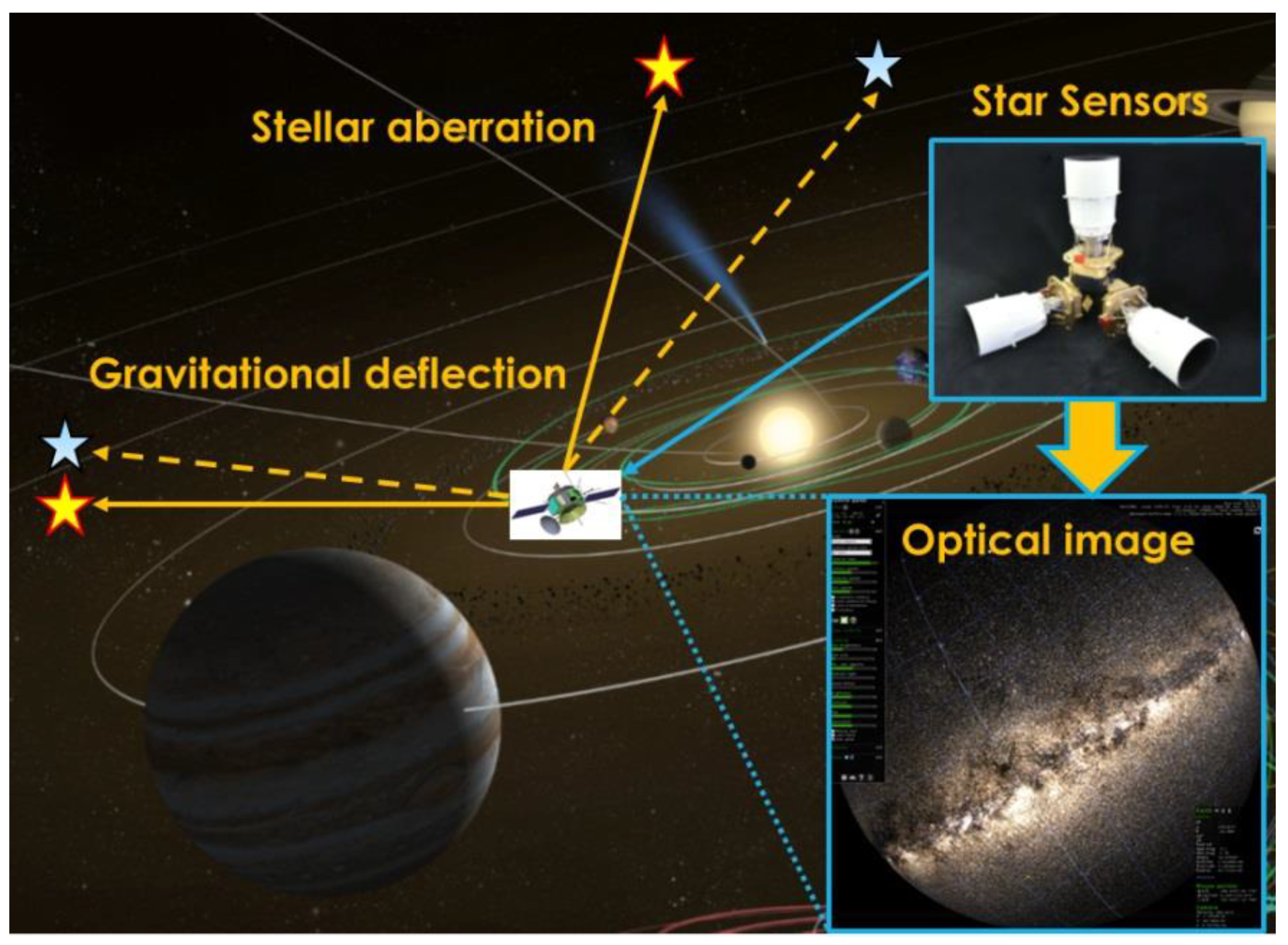
2.1. Basic Principle of Relativistic Navigation
2.2. Dynamic Model
2.3. Measurement Model
3. Navigation Filtering Algorithm
3.1. Extended Kalman Filter
| Algorithm 1: Extended Kalman filter. |
| prediction |
| update |
| 9: end function |
3.2. Q-Learning Approach
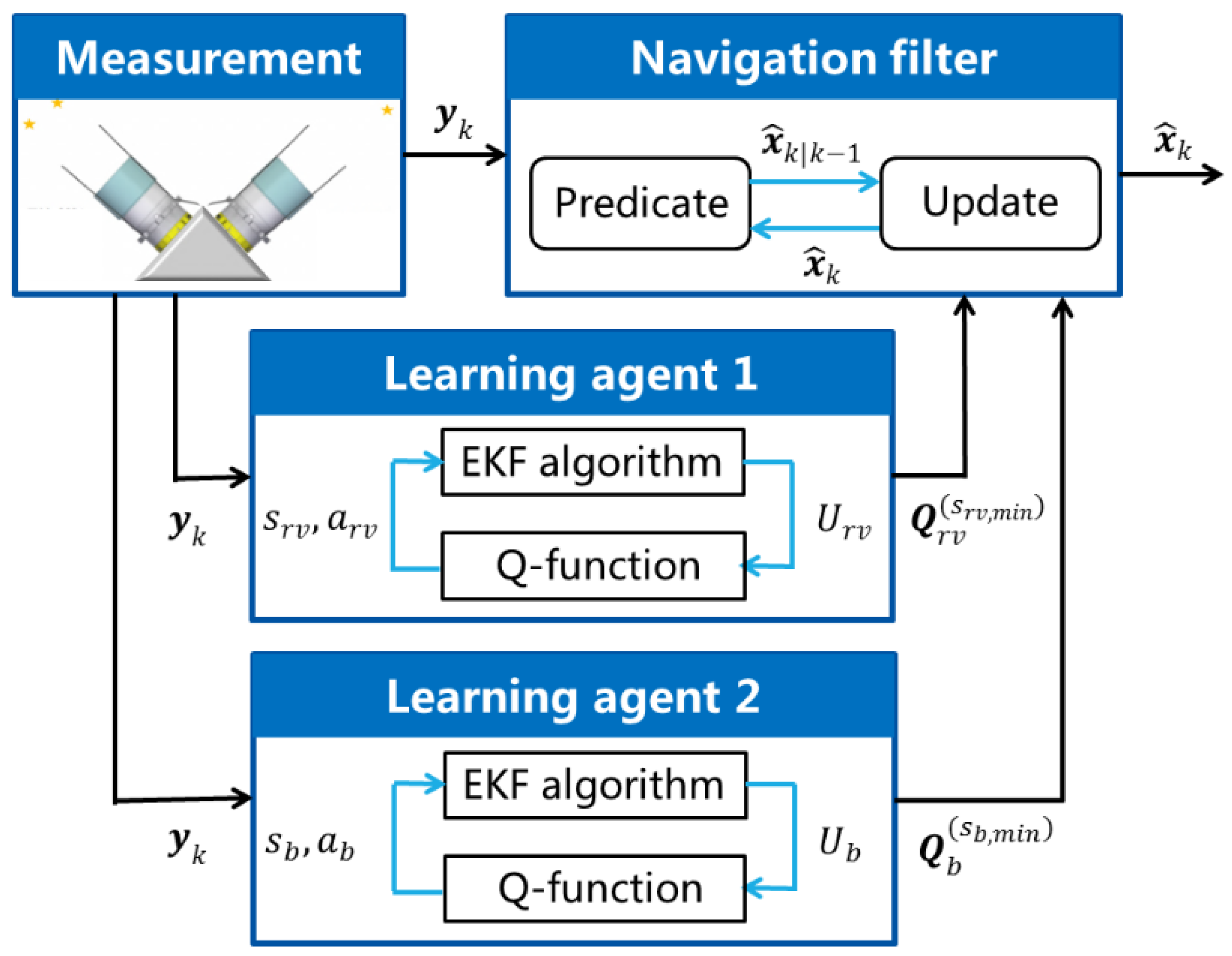
3.3. Parallel Q-Learning Extended Kalman Filter
| Algorithm 2: Parallel Q-learning extended Kalman filter. |
| Input and initial Q-functions and |
| Output |
| , do |
| 4: end |
| , do |
| 8: end |
| , do |
| 14: end |
| 17: end |
| , do |
| 23: end |
| 26: end |
| 30: end |
4. Simulations
4.1. Simulation Conditions
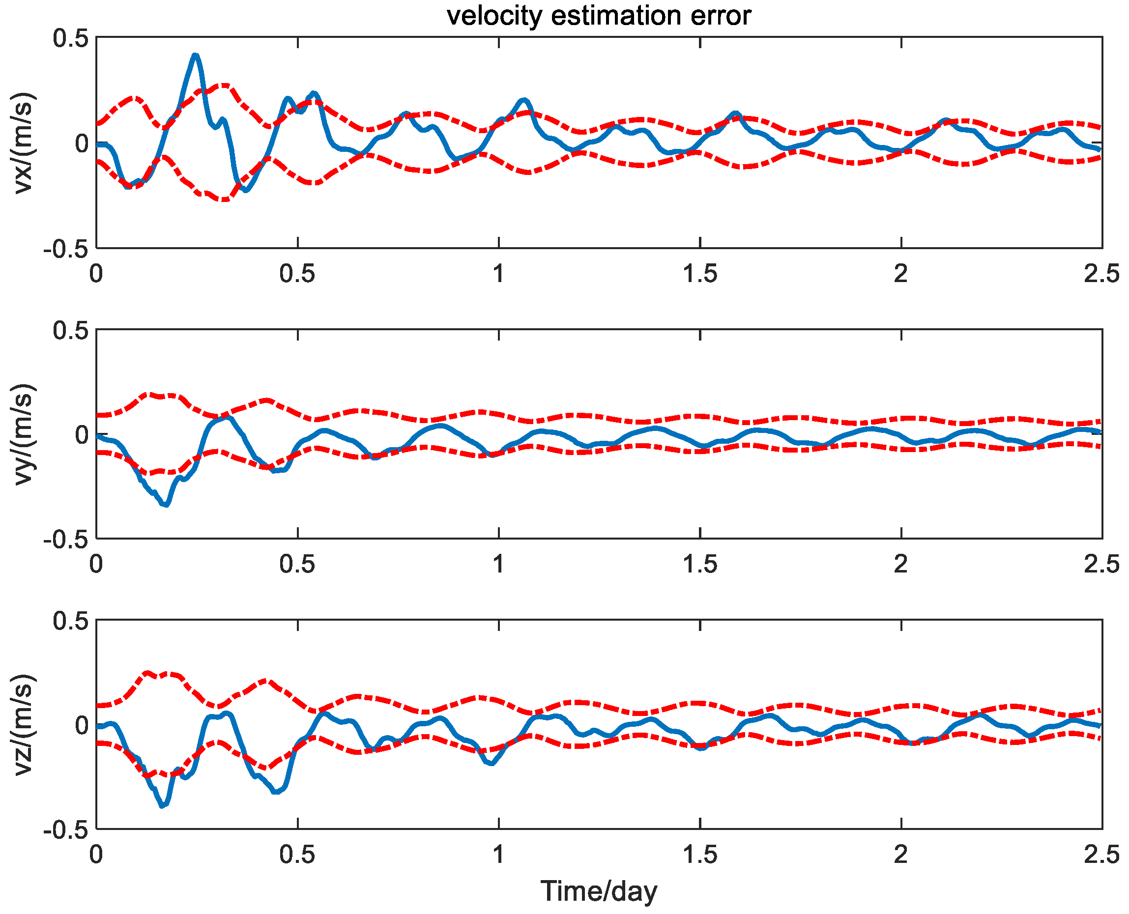
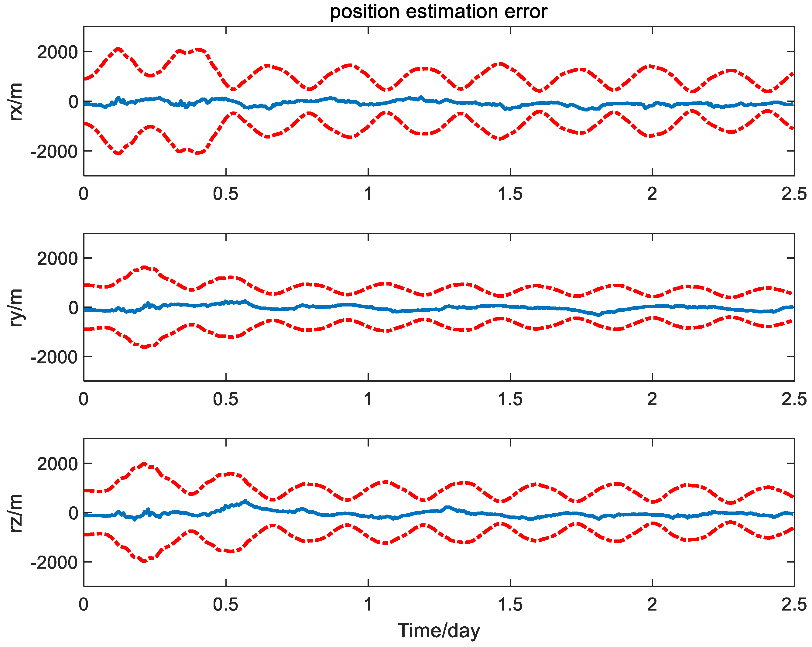
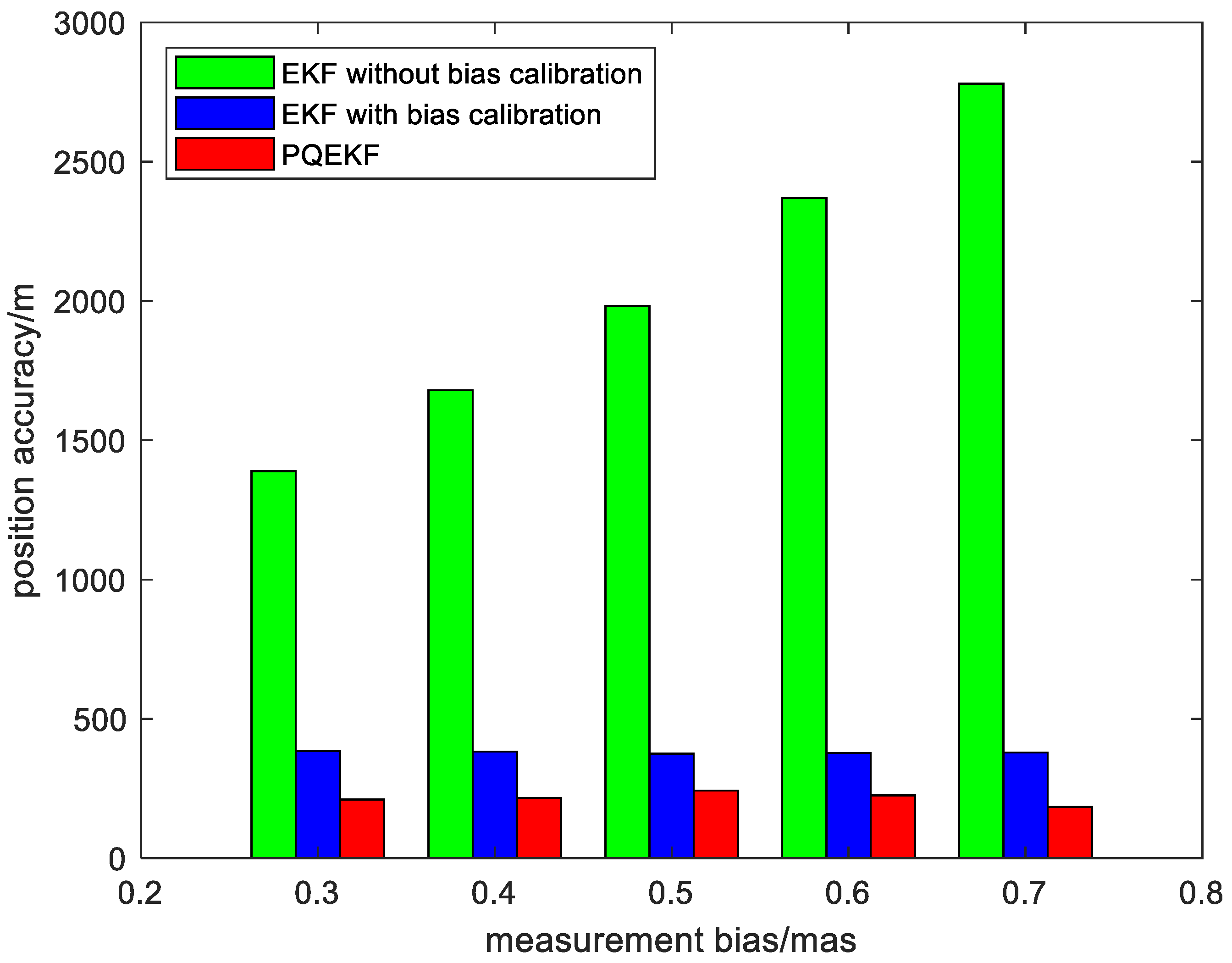
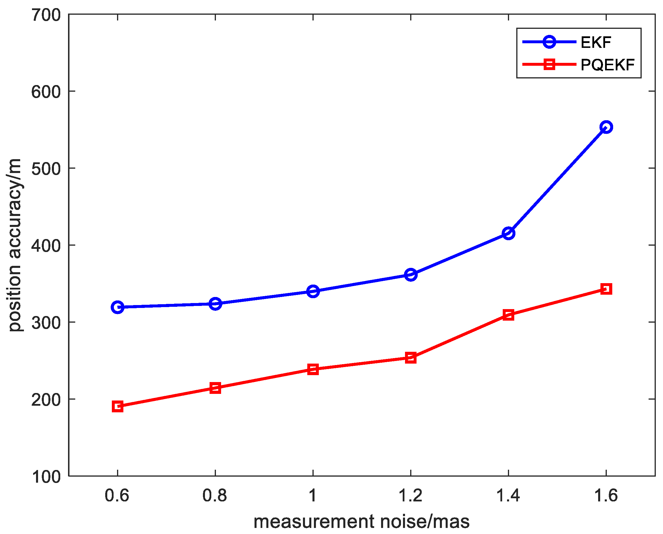
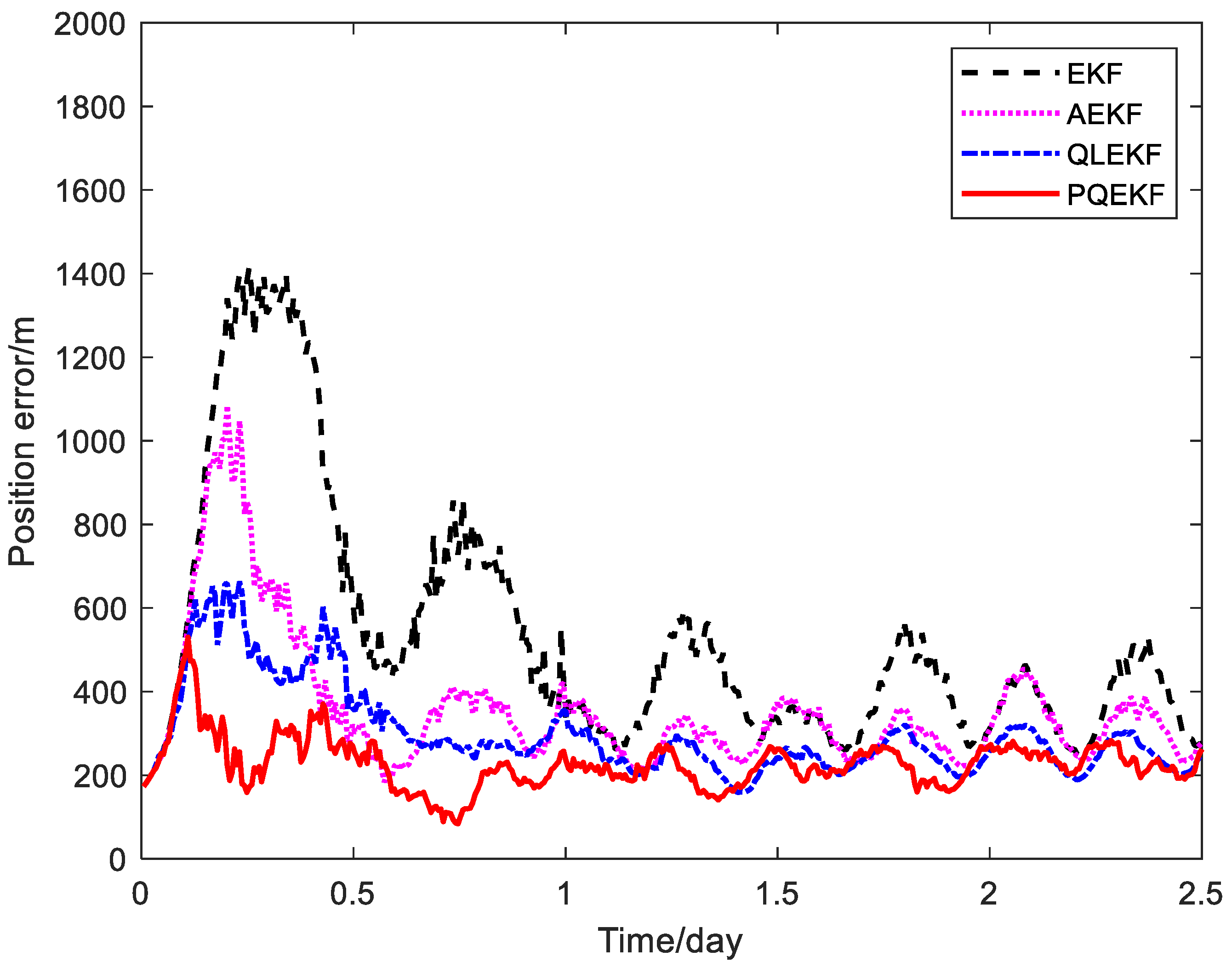
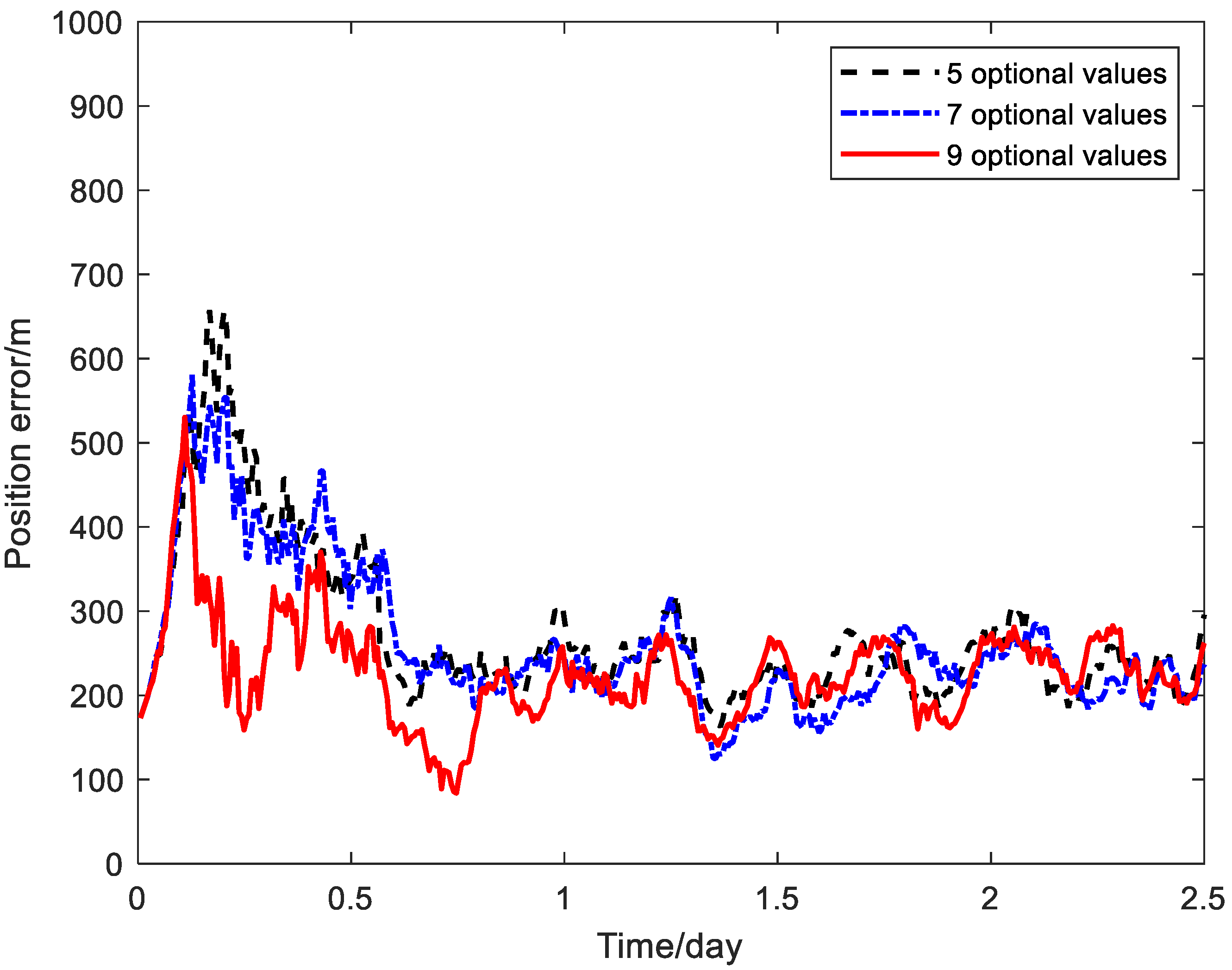
4.2. Simulation Results
5. Conclusions
Author Contributions
Funding
Institutional Review Board Statement
Informed Consent Statement
Data Availability Statement
Conflicts of Interest
Appendix A
Appendix B
Appendix C
Appendix D
Appendix E
References
- Huang, J.; Yang, R.; Zhan, X. Constraint Navigation Filter for Space Vehicle Autonomous Positioning with Deficient GNSS Measurements. Aerosp. Sci. Technol. 2022, 120, 107291. [Google Scholar] [CrossRef]
- Ely, T.A.; Seubert, J.; Bradley, N.; Drain, T.; Bhaskaran, S. Radiometric Autonomous Navigation Fused with Optical for Deep Space Exploration. J. Astronaut. Sci. 2021, 68, 300–325. [Google Scholar] [CrossRef]
- Gallo, E.; Barrientos, A. Reduction of GNSS-Denied Inertial Navigation Errors for Fixed Wing Autonomous Unmanned Air Vehicles. Aerosp. Sci. Technol. 2022, 120, 107237. [Google Scholar] [CrossRef]
- Hu, J.; Liu, J.; Wang, Y.; Ning, X. INS/CNS/DNS/XNAV Deep Integrated Navigation in a Highly Dynamic Environment. Aircr. Eng. Aerosp. Technol. 2023, 95, 180–189. [Google Scholar] [CrossRef]
- Yang, Y.; Han, X.; Song, N.; Wang, Z. A New Method to Improve the Measurement Accuracy of Autonomous Astronomical Navigation. J. Math. 2022, 2022, 3649662. [Google Scholar] [CrossRef]
- Wang, Y.; Yan, T.; Wang, L. Development Situation and Trend of Space Intelligent Navigation Technology. Aerosp. Control Appl. 2022, 48, 9–17. [Google Scholar]
- Zhou, B.; Li, Y.; Zhang, A.; Cui, S. Observability Analysis of Satellite Autonomous Orbit Determination with Modeling and Measurement Errors. Chin. Space Sci. Technol. 2023, 43, 25–34. [Google Scholar]
- Christian, J.A. Optical Navigation Using Planet’s Centroid and Apparent Diameter in Image. J. Guid. Control. Dyn. 2015, 38, 192–204. [Google Scholar] [CrossRef]
- Hou, B.; Wang, J.; Zhou, H.; He, Z.; Li, D.; Liu, X. Guidepost-based Autonomous Orbit Determination Method for GEO Satellite. Adv. Space Res. 2021, 67, 1090–1113. [Google Scholar] [CrossRef]
- Turan, E.; Speretta, S.; Gill, E. Autonomous navigation for deep space small satellites: Scientific and technological advances. Acta Astronaut. 2022, 193, 56–74. [Google Scholar] [CrossRef]
- Sheikh, S.I.; Pines, D.J. Spacecraft Navigation Using X-Ray Pulsars. J. Guid. Control. Dyn. 2006, 29, 49–63. [Google Scholar] [CrossRef]
- Wang, Y.; Zheng, W.; Ge, M.; Zheng, S.; Zhang, S. Use of Statistical Linearization for Nonlinear Least-Squares Problems in Pulsar Navigation. J. Guid. Control. Dyn. 2023, 46, 1850–1855. [Google Scholar] [CrossRef]
- Zoccarato, P.; Larese, S.; Naletto, G.; Zampieri, L.; Brotto, F. Deep Space Navigation by Optical Pulsars. J. Guid. Control. Dyn. 2023, 46, 1501–1511. [Google Scholar] [CrossRef]
- Zhang, W. A Study of the Navigation Technology and Application Based on Astronomical Spectral Velocity Measurement. Navig. Control 2020, 19, 64–73. [Google Scholar]
- Liu, J.; Wang, T.; Ning, X.; Kang, Z. Modelling and analysis of celestial Doppler difference velocimetry navigation considering solar characteristics. IET Radar Sonar Navig. 2020, 14, 1897–1904. [Google Scholar] [CrossRef]
- Gui, M.; Yang, H.; Ning, X.; Ye, W.; Wei, C. A Novel Sun Direction/Solar Disk Velocity Difference Integrated Navigation Method Against Installation Error of Spectrometer Array. IEEE Sens. J. 2023, 23, 17480–17490. [Google Scholar] [CrossRef]
- Christian, J.A. StarNAV: Autonomous Optical Navigation of a Spacecraft by the Relativistic Perturbation of Starlight. Sensors 2019, 19, 4064. [Google Scholar] [CrossRef]
- Bailer-Jones, C.A.L. Lost in Space? Relativistic Interstellar Navigation using an Astrometric Star Catalog. Publ. Astron. Soc. Pac. 2021, 133, 074502. [Google Scholar] [CrossRef]
- McKee, P.; Kowalski, J.; Christian, J. Navigation and star identification for an interstellar mission. Acta Astronaut. 2022, 192, 390–401. [Google Scholar] [CrossRef]
- Klioner, S. A Practical Relativistic Model for Microarcsecond Astrometry in Space. Astron. J. 2003, 125, 1580–1597. [Google Scholar] [CrossRef]
- McKee, P.; Nguyen, H.; Kudenov, M.W.; Christian, J.A. StarNAV with a wide field-of-view optical sensor. Acta Astron. 2022, 197, 220–234. [Google Scholar] [CrossRef]
- Yucalan, D.; Peck, M. Autonomous Navigation of Relativistic Spacecraft in Interstellar Space. J. Guid. Control Dyn. 2021, 44, 1106–1115. [Google Scholar] [CrossRef]
- Xiong, K.; Wei, C. Integrated Celestial Navigation for Spacecraft Using Interferometer and Earth Sensor. Proc. Inst. Mech. Eng. Part G: J. Aerosp. Eng. 2020, 234, 2248–2262. [Google Scholar] [CrossRef]
- Xiong, K.; Wei, C.; Zhou, P. Integrated Autonomous Optical Navigation Using Q-Learning Extended Kalman Filter. Aircr. Eng. Aerosp. Technol. 2022, 94, 848–861. [Google Scholar] [CrossRef]
- Gui, M.; Wei, Y.; Ning, X. Celestial angle measurement navigation for Mars probe considering relativistic effect. J. Deep Space Explor. 2023, 10, 126–132. [Google Scholar]
- Liu, F.; Li, M.; Peng, Y.; Sun, J.; Liu, J. An autonomous navigation method for spacecraft in cislunar space using stellar aberration observation. J. Deep Space Explor. 2023, 10, 159–168. [Google Scholar]
- Ullah, I.; Fayaz, M.; Naveed, N.; Kim, D. ANN Based Learning to Kalman Filter Algorithm for Indoor Environment Prediction in Smart Greenhouse. IEEE Access 2020, 8, 159371–159388. [Google Scholar] [CrossRef]
- Or, B.; Klein, I. A Hybrid Model and Learning-Based Adaptive Navigation Filter. IEEE Trans. Instrum. Meas. 2022, 71, 1–11. [Google Scholar] [CrossRef]
- Ning, X.; Li, Z.; Wu, W.; Yang, Y.; Fang, J.; Liu, G. Recursive Adaptive Filter Using Current Innovation for Celestial Navigation During the Mars Approach Phase. Sci. China-Inf. Sci. 2017, 60, 032205. [Google Scholar] [CrossRef]
- Li, W.; Sun, S.; Jia, Y.; Du, J. Robust unscented Kalman filter with adaptation of process and measurement noise covariances. Digit. Signal Process. 2016, 48, 93–103. [Google Scholar] [CrossRef]
- Jia, W.; Tian, Y.; Duan, H.; Luo, R.; Lian, J.; Ruan, C.; Zhao, D.; Li, C. Autonomous Navigation Control Based on Improved Adaptive Filtering for Agricultural Robot. Int. J. Adv. Robot. Syst. 2020, 17, 1729881420925357. [Google Scholar] [CrossRef]
- Xiong, K.; Zhou, P.; Wei, C. Autonomous Navigation of Unmanned Aircraft Using Space Target LOS Measurements and QLEKF. Sensors 2022, 22, 6992. [Google Scholar] [CrossRef] [PubMed]
- Tao, W.; Zhang, J.; Hu, H.; Zhang, J.; Sun, H.; Zeng, Z.; Song, J.; Wang, J. Intelligent Navigation for the Cruise Phase of Solar System Boundary Exploration Based on Q-learning EKF. Complex Intell. Syst. 2024, 2, 2653–2672. [Google Scholar] [CrossRef]
- Xiong, K.; Wei, C.; Zhang, H. Q-learning for noise covariance adaptation in extended Kalman filter. Asian J. Control. 2021, 23, 1803–1816. [Google Scholar] [CrossRef]
- Chen, C.; Wu, X.; Bo, Y.; Chen, Y.; Liu, Y.; Alsaadi, F.E. SARSA in extended Kalman Filter for complex urban environments positioning. Int. J. Syst. Sci. 2021, 52, 3044–3059. [Google Scholar] [CrossRef]
- Yin, Y.; Li, S.E.; Tang, K.; Cao, W.; Wu, W.; Li, H. Approximate optimal filter design for vehicle system through Actor-Critic reinforcement learning. Automot. Innov. 2022, 5, 415–426. [Google Scholar] [CrossRef]
- Crassidis, J.L.; Markley, F.L.; Cheng, Y. Survey of Nonlinear Attitude Estimation Methods. J. Guid. Control. Dyn. 2007, 30, 12–28. [Google Scholar] [CrossRef]
- Hu, Z.; Gong, W. Constrained Evolutionary Optimization Based on Reinforcement Learning Using the Objective Function and Constraints. Knowl.-Based Syst. 2022, 237, 107731. [Google Scholar] [CrossRef]
- Jang, B.; Kim, M.; Harerimana, G.; Kim, J.W. Q-learning Algorithms: A Comprehensive Classification and Applications. IEEE Access 2019, 7, 133653–133667. [Google Scholar] [CrossRef]
- Li, Y.; Yang, C.; Hou, Z.; Feng, Y.; Yin, C. Data-driven approximate Q-learning stabilization with optimality error bound analysis. Automatica 2019, 103, 435–442. [Google Scholar] [CrossRef]
- Shi, H.; Li, X.; Hwang, K.; Pan, W.; Xu, G. Decoupled Visual Servoing with Fuzzy Q-learning. IEEE Trans. Ind. Inform. 2018, 14, 241–252. [Google Scholar] [CrossRef]
- Wu, G. UAV-Based Interference Source Localization: A Multi-model Q-learning Approach. IEEE Access 2019, 7, 137982–137991. [Google Scholar] [CrossRef]
- Maia, R.; Mendes, J.; Araujo, R.; Silva, M.; Nunes, U. Regenerative Braking System Modeling by Fuzzy Q-Learning. Eng. Appl. Artif. Intell. 2020, 93, 103712. [Google Scholar] [CrossRef]
- Wei, Q.; Lewis, F.L.; Sun, Q.; Yan, P.; Song, R. Discrete-time Deterministic Q-learning: A Novel Convergence Analysis. IEEE Trans. Cybern. 2017, 47, 1224–1237. [Google Scholar] [CrossRef]


| Simulation conditions | Duration of simulation | 2.5 days |
| Measurement noise standard deviation | 1 mas | |
| Measurement bias | 0.3 mas | |
| Update frequency | 0.1 Hz | |
| EKF parameters | Initial estimation error covariance | |
| Process noise covariance | ||
| Measurement noise covariance | ||
| PQEKF parameters | State space for agent 1 | |
| State space for agent 2 | ||
| Window size | ||
| Discounted factor |
| Calibration Method | Average RMS Error | ||
|---|---|---|---|
| Position (m) | Velocity (m/s) | Measurement Bias (mas) | |
| EKF | 609.8 | 0.073 | 0.275 |
| AEKF | 371.1 | 0.045 | 0.187 |
| QLEKF | 328.3 | 0.036 | 0.088 |
| PQEKF | 215.5 | 0.025 | 0.055 |
Disclaimer/Publisher’s Note: The statements, opinions and data contained in all publications are solely those of the individual author(s) and contributor(s) and not of MDPI and/or the editor(s). MDPI and/or the editor(s) disclaim responsibility for any injury to people or property resulting from any ideas, methods, instructions or products referred to in the content. |
© 2024 by the authors. Licensee MDPI, Basel, Switzerland. This article is an open access article distributed under the terms and conditions of the Creative Commons Attribution (CC BY) license (https://creativecommons.org/licenses/by/4.0/).
Share and Cite
Xiong, K.; Zhao, Q.; Yuan, L. Calibration Method for Relativistic Navigation System Using Parallel Q-Learning Extended Kalman Filter. Sensors 2024, 24, 6186. https://doi.org/10.3390/s24196186
Xiong K, Zhao Q, Yuan L. Calibration Method for Relativistic Navigation System Using Parallel Q-Learning Extended Kalman Filter. Sensors. 2024; 24(19):6186. https://doi.org/10.3390/s24196186
Chicago/Turabian StyleXiong, Kai, Qin Zhao, and Li Yuan. 2024. "Calibration Method for Relativistic Navigation System Using Parallel Q-Learning Extended Kalman Filter" Sensors 24, no. 19: 6186. https://doi.org/10.3390/s24196186
APA StyleXiong, K., Zhao, Q., & Yuan, L. (2024). Calibration Method for Relativistic Navigation System Using Parallel Q-Learning Extended Kalman Filter. Sensors, 24(19), 6186. https://doi.org/10.3390/s24196186