Figure 1.
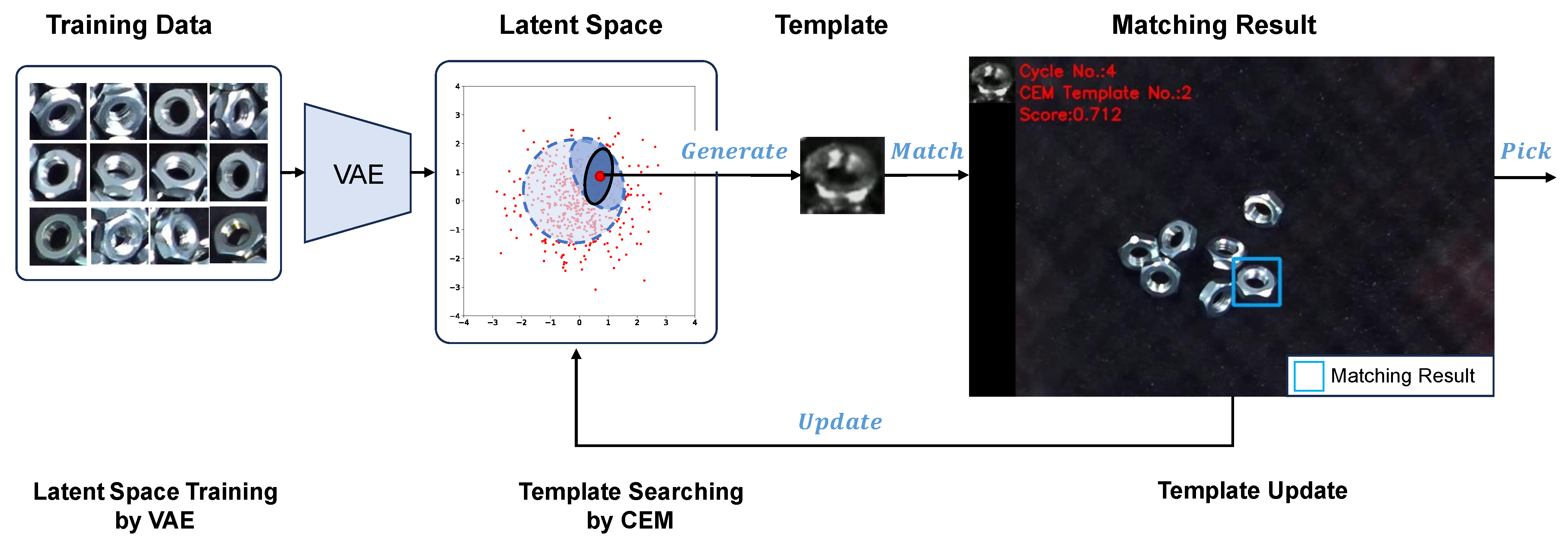
The framework of a variational template generation control system. Firstly, utilizing a VAE to train a low-dimensional latent space to represent the templates’ feature map of the training data. Then, employing a CEM to identify an adaptive template within the latent space. Lastly, updating the template based on its matching performance feedback. In the bin-picking task, the image changes after each object is picked. If the current template’s matching performance falls below a predefined threshold, the template will be updated based on the current camera’s frame.
Figure 1.
The framework of a variational template generation control system. Firstly, utilizing a VAE to train a low-dimensional latent space to represent the templates’ feature map of the training data. Then, employing a CEM to identify an adaptive template within the latent space. Lastly, updating the template based on its matching performance feedback. In the bin-picking task, the image changes after each object is picked. If the current template’s matching performance falls below a predefined threshold, the template will be updated based on the current camera’s frame.
Figure 2.
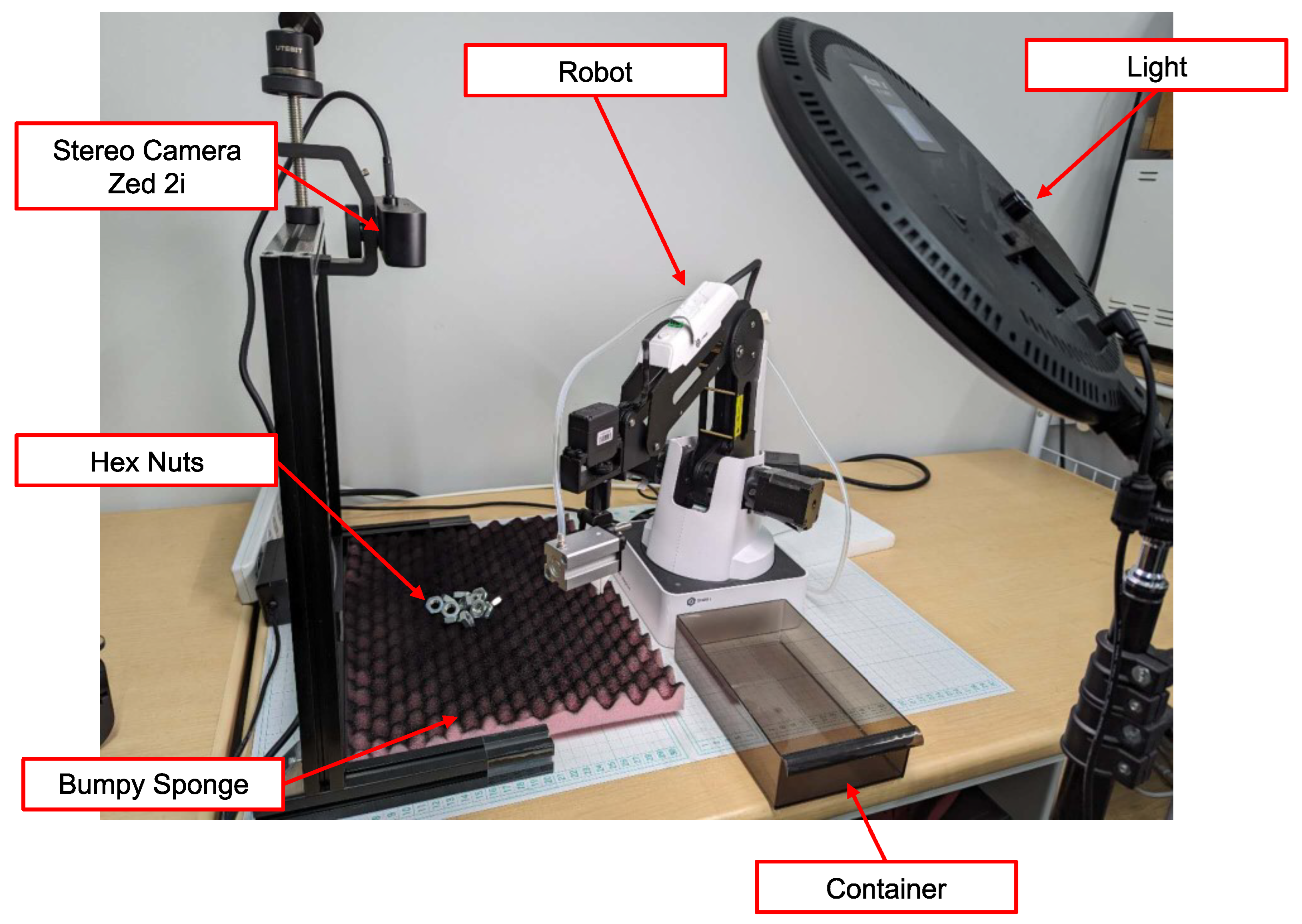
Environmental setup. Hex nuts were utilized as the research subject of the study. To demonstrate various poses, a bumpy sponge served as the foundation. Image capture and depth detection were facilitated by a stereo camera system. The lux level of the workspace was set as 1200 lux.
Figure 2.
Environmental setup. Hex nuts were utilized as the research subject of the study. To demonstrate various poses, a bumpy sponge served as the foundation. Image capture and depth detection were facilitated by a stereo camera system. The lux level of the workspace was set as 1200 lux.
Figure 3.
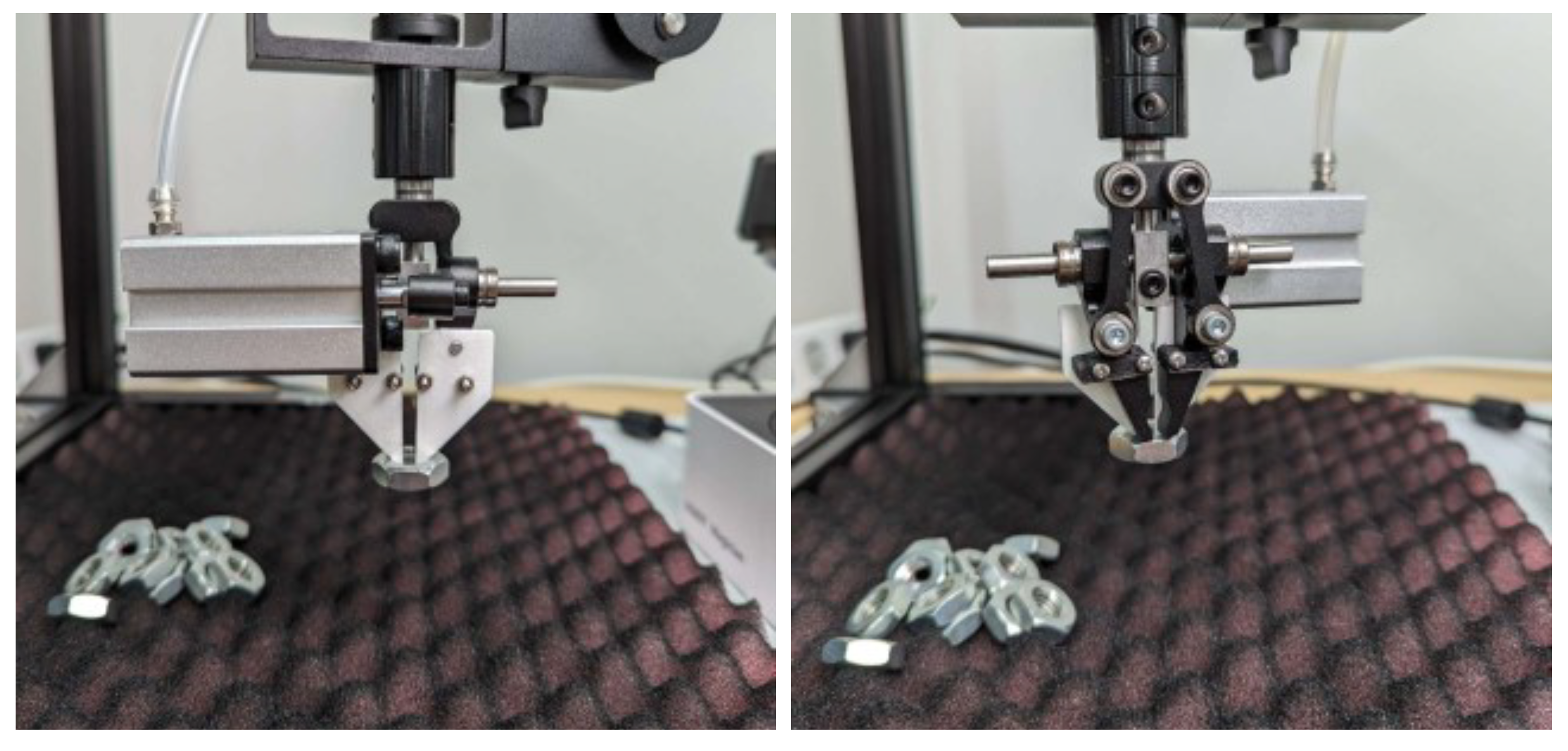
Grippers designed for nut grasping.
Figure 3.
Grippers designed for nut grasping.
Figure 4.
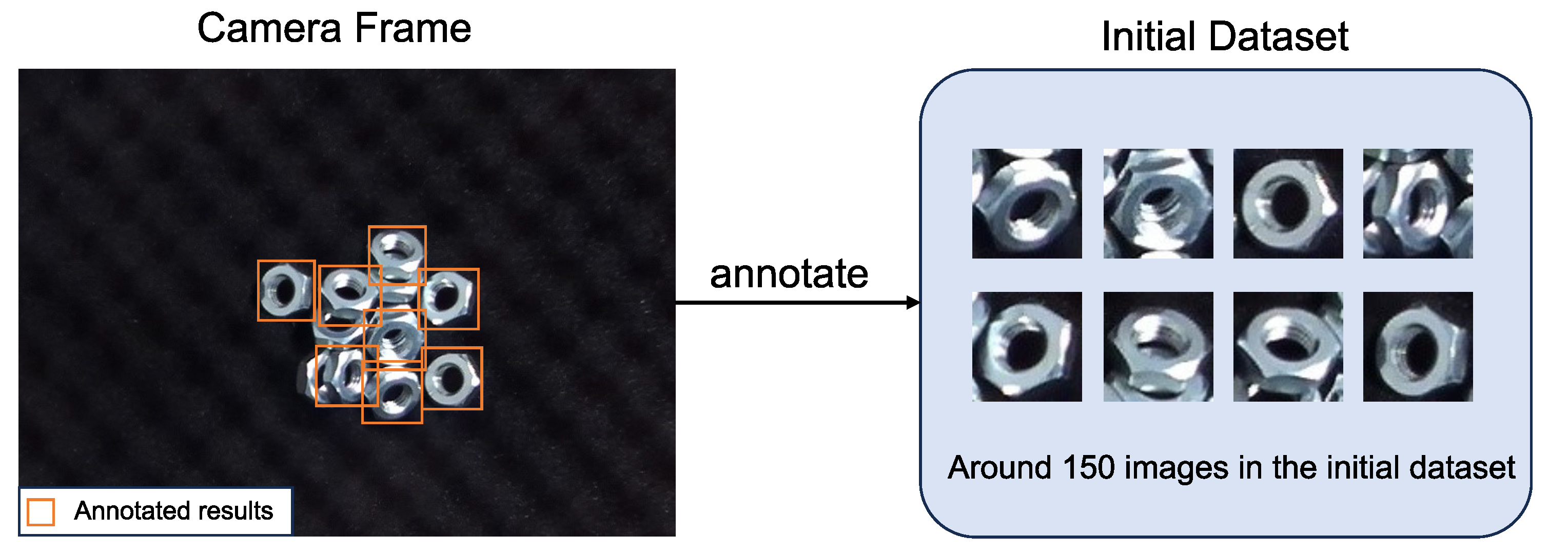
Assisted-manual data collection stage. In this stage, operators are directly involved in annotating objects in the initial dataset. An object that can be grasped by the robot will be annotated. Additionally, when the model fails to detect objects in certain scenes, manual annotation is used to collect data for those instances.
Figure 4.
Assisted-manual data collection stage. In this stage, operators are directly involved in annotating objects in the initial dataset. An object that can be grasped by the robot will be annotated. Additionally, when the model fails to detect objects in certain scenes, manual annotation is used to collect data for those instances.
Figure 5.
Semi-automatic data collection stage. In this stage, the model is deployed to automatically detect objects. However, due to potential limitations in the model’s performance, human verification is required to confirm the accuracy of the detected objects. Any discrepancies or inaccuracies identified during this process are annotated and corrected to ensure the quality of the training dataset.
Figure 6.
The architecture of a VAE training model. Input: grayscale image. Encoder: 5 convolutional layers with ReLU activation, and the last convolutional layer is flattened as a 2048-neuron fc layer. Latent vector z is 4-dimensional, obtained by 2 fc layers representing mean and variance using the reparameterization trick. Decoder: Latent vector mapped to a 2048-neuron fc layer, then reshaped to size by using the “view” function of the Pytorch. Followed by 5 deconvolutional layers with ReLU activation. The last deconvolutional layer is activated by Sigmoid to obtain the output image. Output: grayscale image.
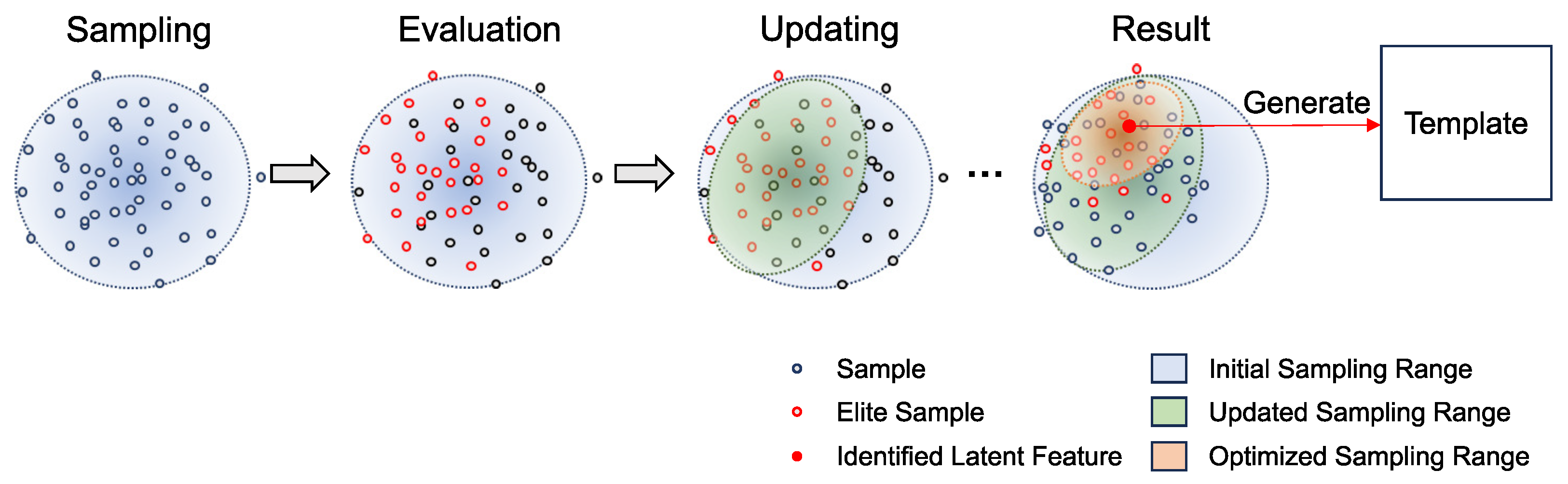
Figure 7.
The template searching process by CEM. The search process by CEM involves sampling, evaluation, and updating. Sampling: samples are drawn from a Gaussian distribution. Evaluation: each sample point is evaluated, and elite samples are selected based on their evaluation results. Updating: the sampling range is updated based on the elite samples. This process is repeated until the sampling range becomes smaller than a predefined threshold. The mean of the optimized sampling range is then used as the identified latent feature to generate the template for matching.
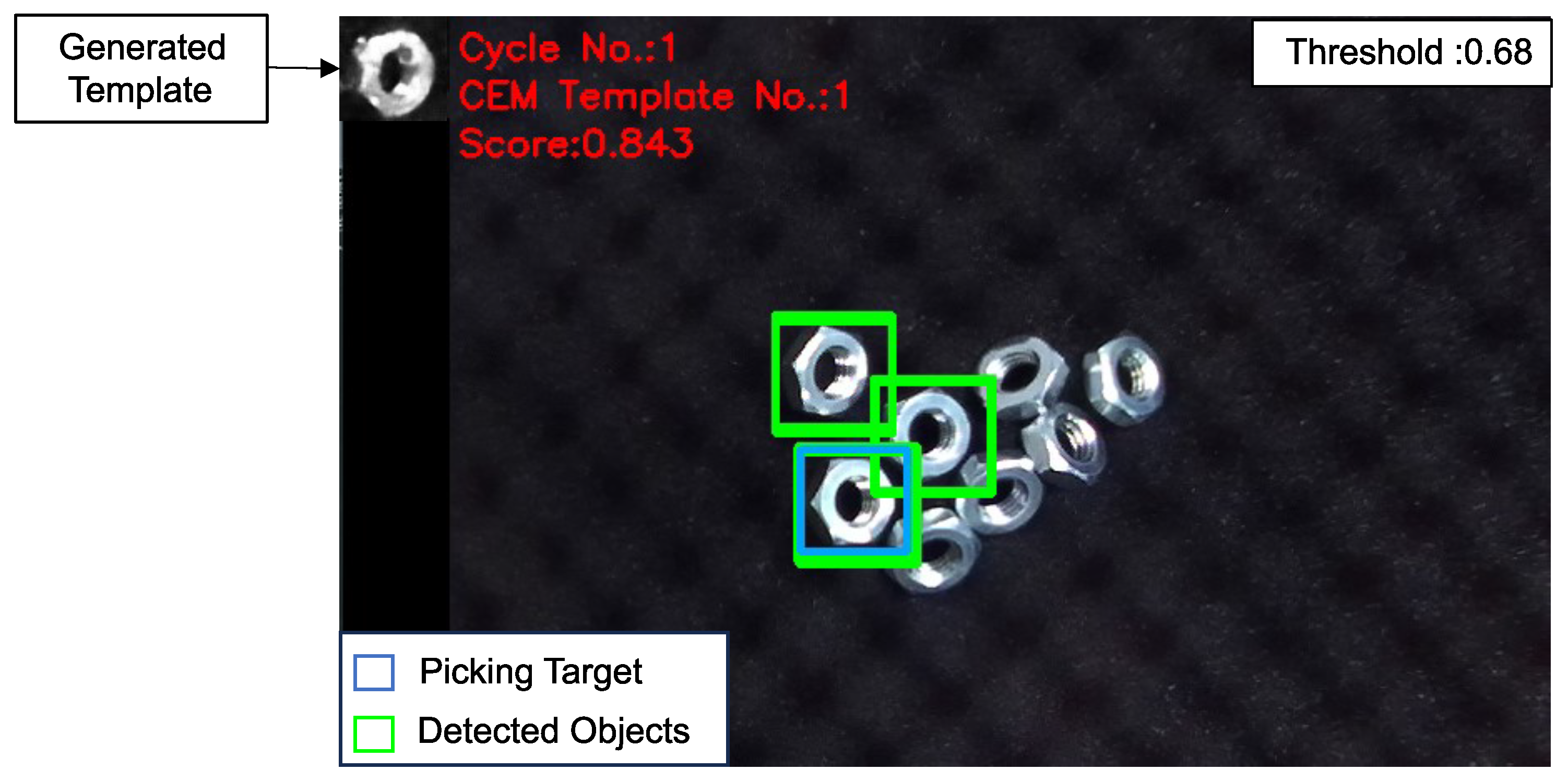
Figure 8.
Generated template and its matching result. The green windows indicate the detected objects with a matching score above the threshold of 0.68. Meanwhile, the blue window highlights the location with the highest matching score, serving as the picking target for the robot.
Figure 8.
Generated template and its matching result. The green windows indicate the detected objects with a matching score above the threshold of 0.68. Meanwhile, the blue window highlights the location with the highest matching score, serving as the picking target for the robot.
Figure 9.
Searching process in latent space. In the figure, represents each dimension of the latent space, the green point shows the start, and the red star shows the finish.
Figure 9.
Searching process in latent space. In the figure, represents each dimension of the latent space, the green point shows the start, and the red star shows the finish.
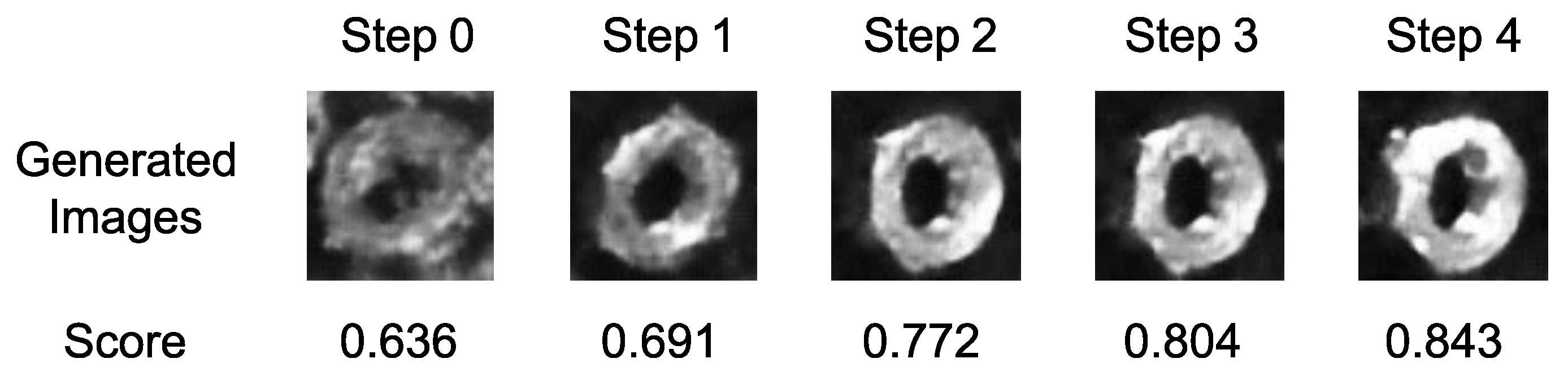
Figure 10.
The series of generated templates and their corresponding matching scores at each searching step. Initially, the start latent vector produces an image of the nut with unclear features. As the CEM progresses, the generated image evolves, and its matching score increases.
Figure 10.
The series of generated templates and their corresponding matching scores at each searching step. Initially, the start latent vector produces an image of the nut with unclear features. As the CEM progresses, the generated image evolves, and its matching score increases.
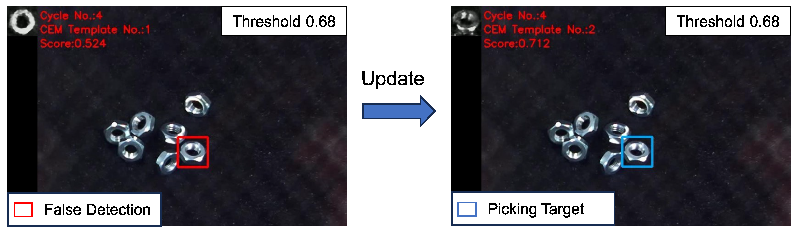
Figure 11.
Example of template updating during robot bin-picking. The previous template was generated as planned, but the objects in the image were all tilted, resulting in false-negative detection (the matching score was 0.524, smaller than the threshold of 0.68). After the template was updated using the CEM method, the matching performance improved significantly, with a matching score of 0.712, indicating successful object detection.
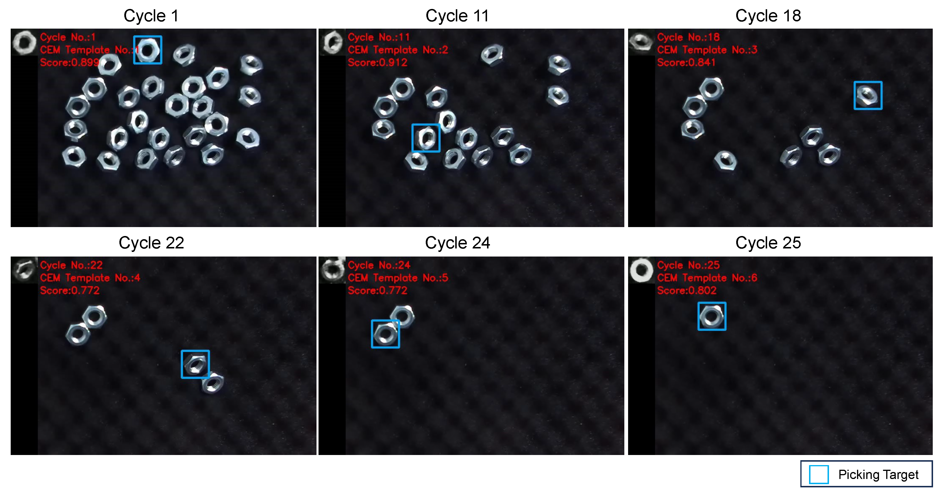
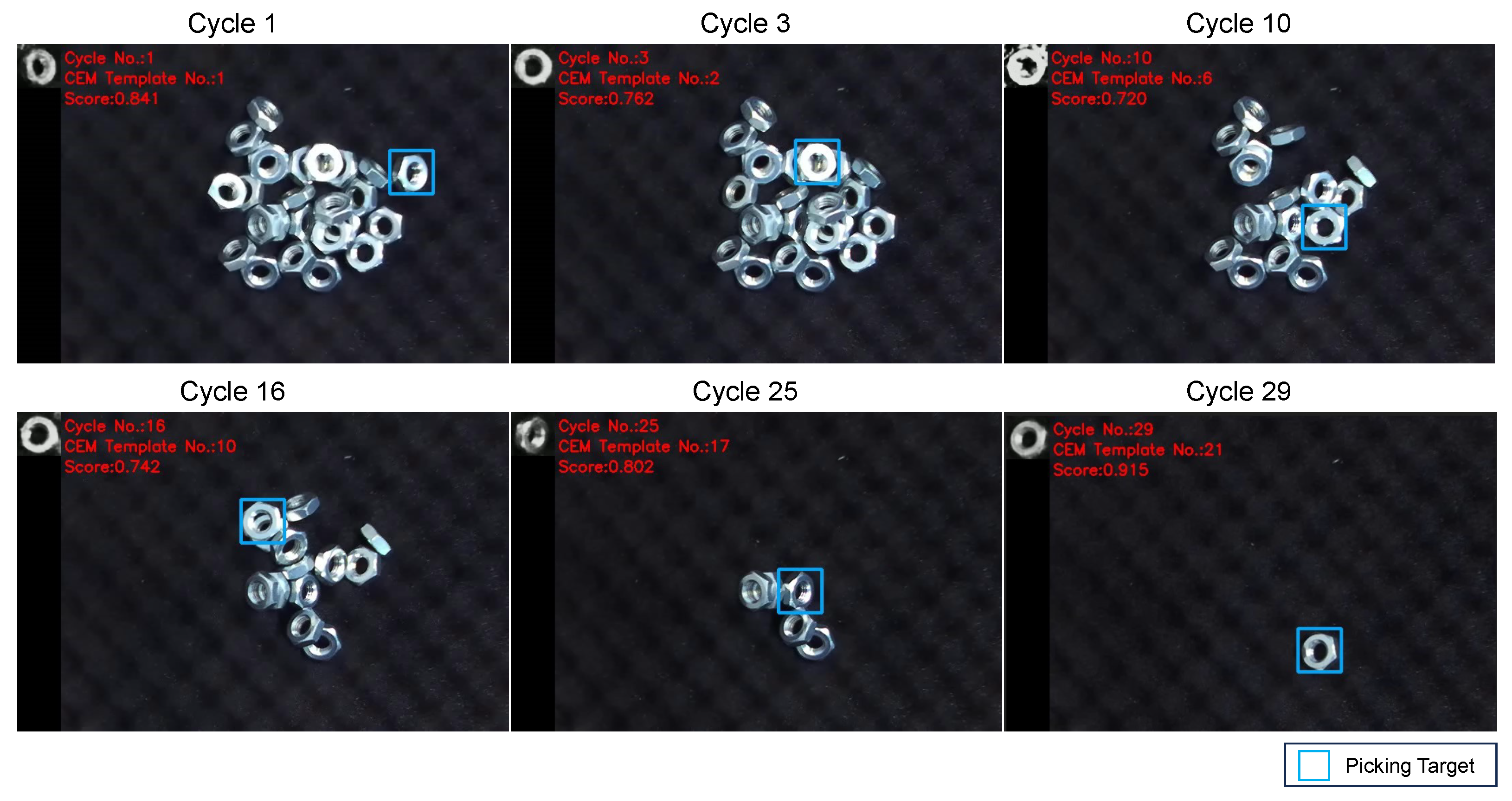
Figure 12.
Snapshots of the experiment with different object’s poses. In the experiment, all the objects were successfully detected and picked up.
Figure 12.
Snapshots of the experiment with different object’s poses. In the experiment, all the objects were successfully detected and picked up.
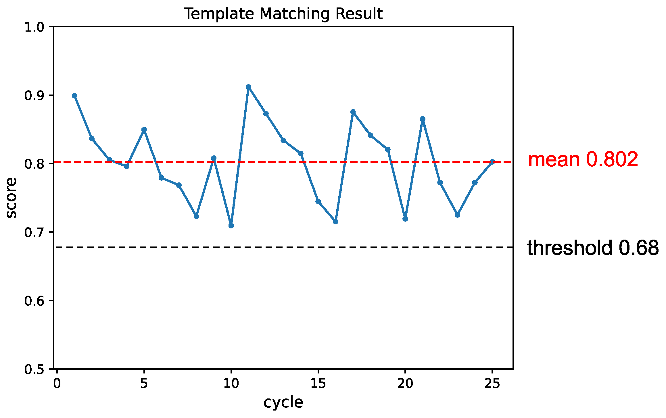
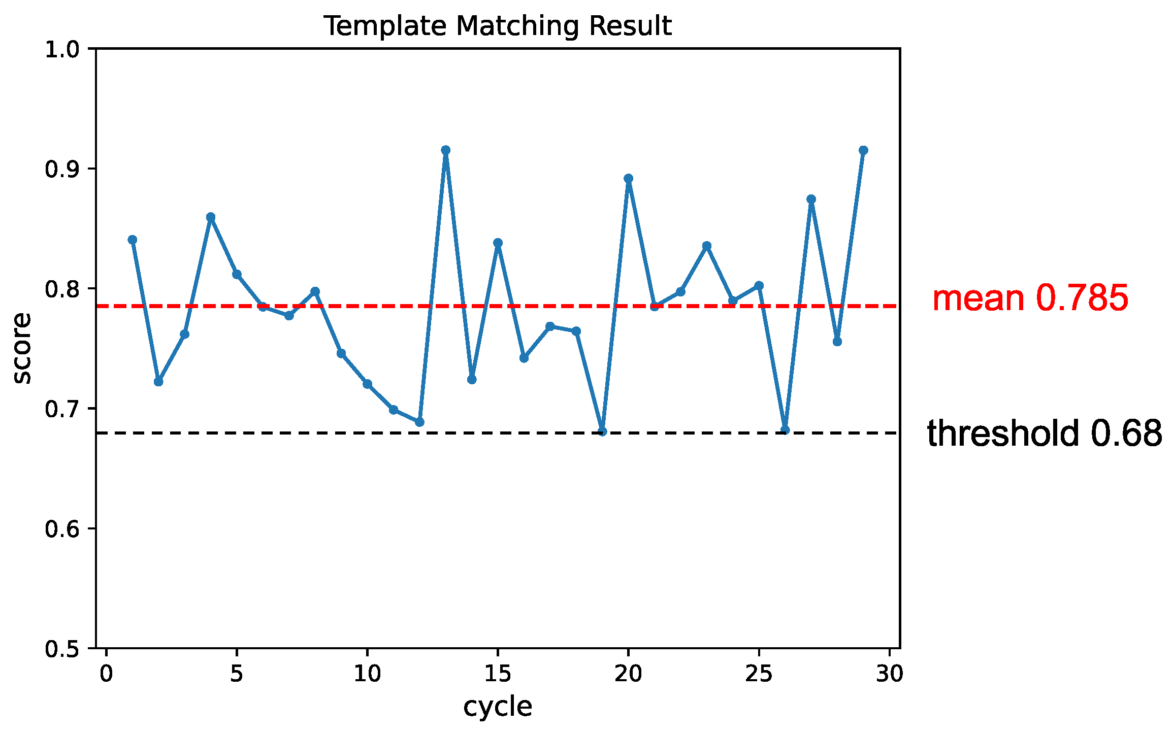
Figure 13.
The change in matching score throughout the experiment. Each instance where an object was detected and picked up was considered one cycle. The template was updated whenever the matching score fell below the threshold, leading to a subsequent recovery in the matching result.
Figure 13.
The change in matching score throughout the experiment. Each instance where an object was detected and picked up was considered one cycle. The template was updated whenever the matching score fell below the threshold, leading to a subsequent recovery in the matching result.
Figure 14.
Snapshots of the experiment with varying background appearances. The significant variations in each window candidate necessitated frequent updates to the template.
Figure 14.
Snapshots of the experiment with varying background appearances. The significant variations in each window candidate necessitated frequent updates to the template.
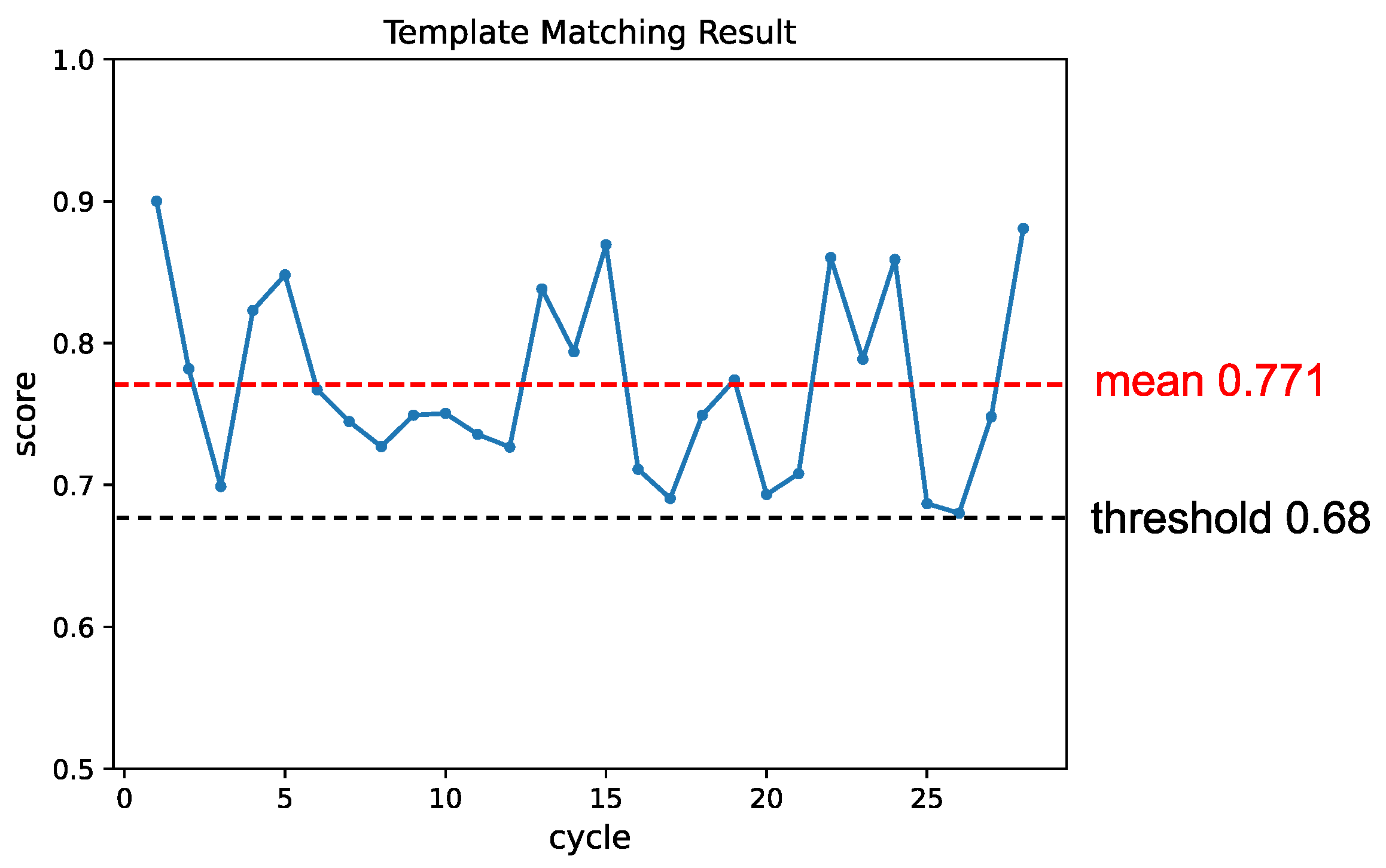
Figure 15.
The change in matching score throughout the experiment in varying background appearance conditions. Similarly to the pose condition experiment, the template was updated whenever the matching score dropped below the threshold, resulting in subsequent improvements in the matching results.
Figure 15.
The change in matching score throughout the experiment in varying background appearance conditions. Similarly to the pose condition experiment, the template was updated whenever the matching score dropped below the threshold, resulting in subsequent improvements in the matching results.
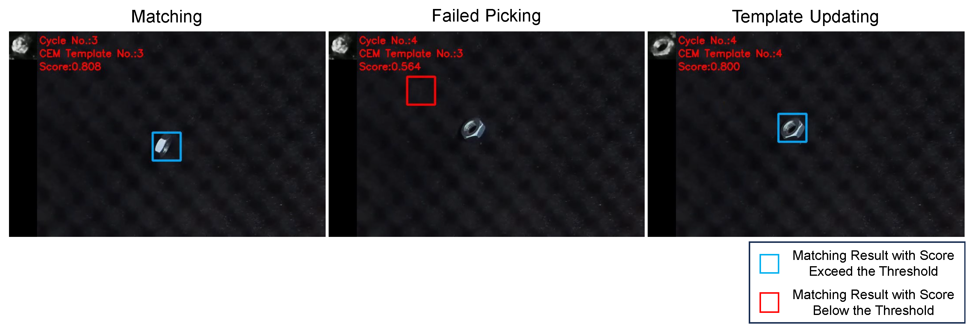
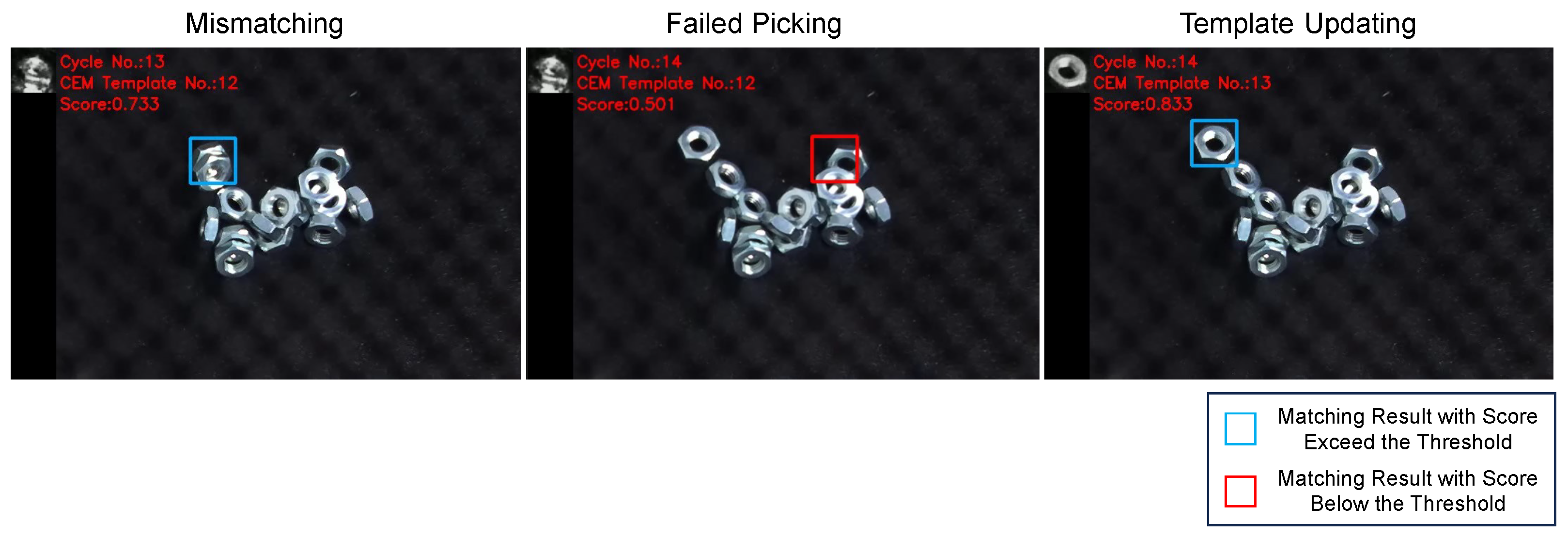
Figure 16.
Snapshots of object detection and picking process in a vertical pose. Matching: As the vertical pose was untrained, the proposed method generated templates with similar features but did not accurately resemble the shape of a nut. Despite this discrepancy, the template detected the object. Failed Picking: Due to the limitation of the robot’s gripper, the robot knocked down the nut. Template Updating: Since the object’s pose changed and the matching score fell below the threshold, the template was updated accordingly, and the robot proceeded to pick up the nut.
Figure 17.
A failed grasping attempt case by low-precision matching result. Mismatching: The NCC similarity measure does not effectively capture the spatial relationships between objects and led to failure. Failed Picking: The robot failed to grasp the nut accurately, causing it to move. Template Updating: The template was updated, improving the matching result.
Figure 18.
Experimental setup with additional lighting source. In addition to the existing lighting conditions, we introduced an additional light source. Furthermore, we altered the color of this additional light to provide a variation from the training environment. The lux level was increased to 1500.
Figure 19.
Snapshots of the experiment with an additional lighting source. Despite the change in lighting condition, the object was successfully detected and grasped.
Figure 19.
Snapshots of the experiment with an additional lighting source. Despite the change in lighting condition, the object was successfully detected and grasped.
Figure 20.
The change in matching score throughout the experiment of lighting condition. Similar to the conditions of pose and background, the template was updated whenever the matching score fell below the threshold, resulting in a subsequent recovery in the matching result.
Figure 20.
The change in matching score throughout the experiment of lighting condition. Similar to the conditions of pose and background, the template was updated whenever the matching score fell below the threshold, resulting in a subsequent recovery in the matching result.
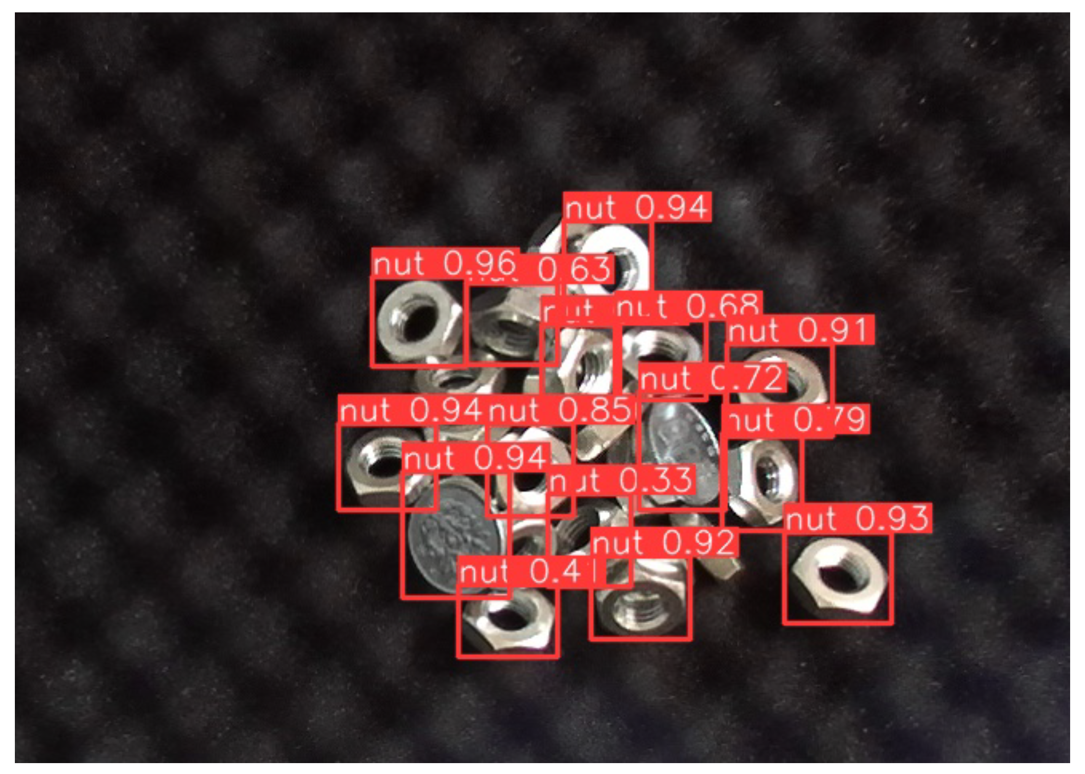
Figure 21.
YOLO’s detection results with 100-yen coin. Coins were mistakenly identified as nuts, with confidence scores exceeding 0.90, even higher than those for actual nuts. Additionally, for some nuts, the model failed to achieve a confidence score above the 0.5 threshold.
Figure 21.
YOLO’s detection results with 100-yen coin. Coins were mistakenly identified as nuts, with confidence scores exceeding 0.90, even higher than those for actual nuts. Additionally, for some nuts, the model failed to achieve a confidence score above the 0.5 threshold.
Figure 22.
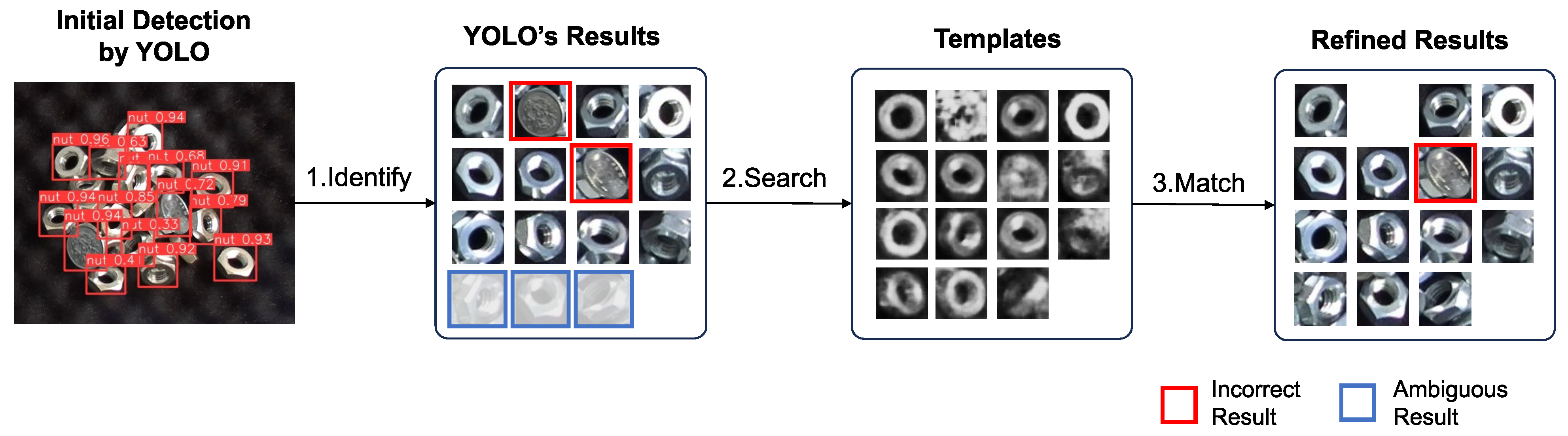
YOLO’s detection results refining process by templates generated via latent space searching. The process involves three steps: (1) Initial detection by YOLO: YOLO identifies potential detection target windows. Incorrect results and ambiguous results which the confidence score under the threshold were observed. (2) Template search based on YOLO’s results: for each potential target, a corresponding template is searched in the trained latent space. (3) Matching with templates: YOLO’s results were refined by template matching. Matches with scores below the threshold are filtered out. Although one different object could not be filtered out by the threshold, its YOLO detection result with a confidence score of 0.717 was refined to a template matching score of 0.567, bringing it closer to the ground truth.
Figure 22.
YOLO’s detection results refining process by templates generated via latent space searching. The process involves three steps: (1) Initial detection by YOLO: YOLO identifies potential detection target windows. Incorrect results and ambiguous results which the confidence score under the threshold were observed. (2) Template search based on YOLO’s results: for each potential target, a corresponding template is searched in the trained latent space. (3) Matching with templates: YOLO’s results were refined by template matching. Matches with scores below the threshold are filtered out. Although one different object could not be filtered out by the threshold, its YOLO detection result with a confidence score of 0.717 was refined to a template matching score of 0.567, bringing it closer to the ground truth.
Figure 23.
Template searching process in latent space by CEM. Each CEM optimization step consists of three processes: sampling, evaluation, and updating. After several CEM optimization steps, if no template is found that results in a template matching score exceeding the threshold the input image can be considered as not the target object.
Figure 24.
Precision–recall curves of two methods. The precision–recall curves of the two methods show that YOLO achieved an AP of 0.629, while our hybrid method achieved an AP of 0.944. The hybrid method achieved higher precision and recall than YOLO, demonstrating its better performance compared to YOLO.
Figure 25.
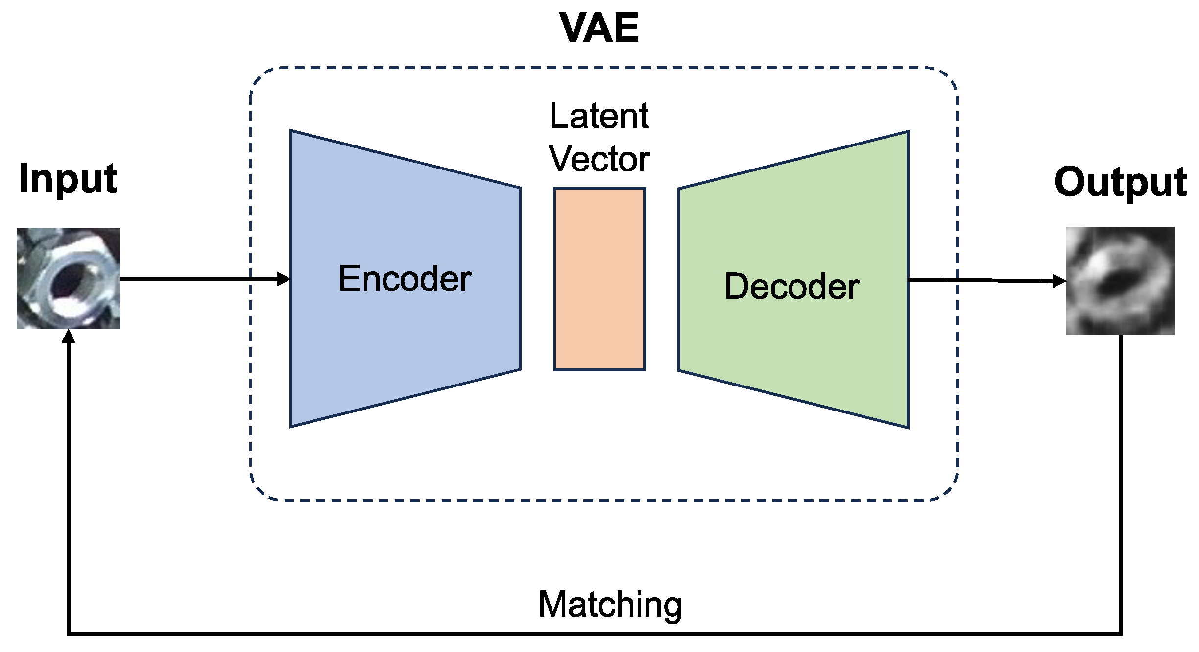
The VAE reconstruction approach for abnormal detection. An untrained input can be reconstructed to resemble the VAE’s training data. By matching the input and the output, it can be determined whether the input belongs to the training domain or not. However, an object with an untrained factor combination can also cause a lower matching score, which may affect detection performance. In the figure, the matching score is 0.410, which is below the threshold of 0.5.
Figure 25.
The VAE reconstruction approach for abnormal detection. An untrained input can be reconstructed to resemble the VAE’s training data. By matching the input and the output, it can be determined whether the input belongs to the training domain or not. However, an object with an untrained factor combination can also cause a lower matching score, which may affect detection performance. In the figure, the matching score is 0.410, which is below the threshold of 0.5.
Figure 26.
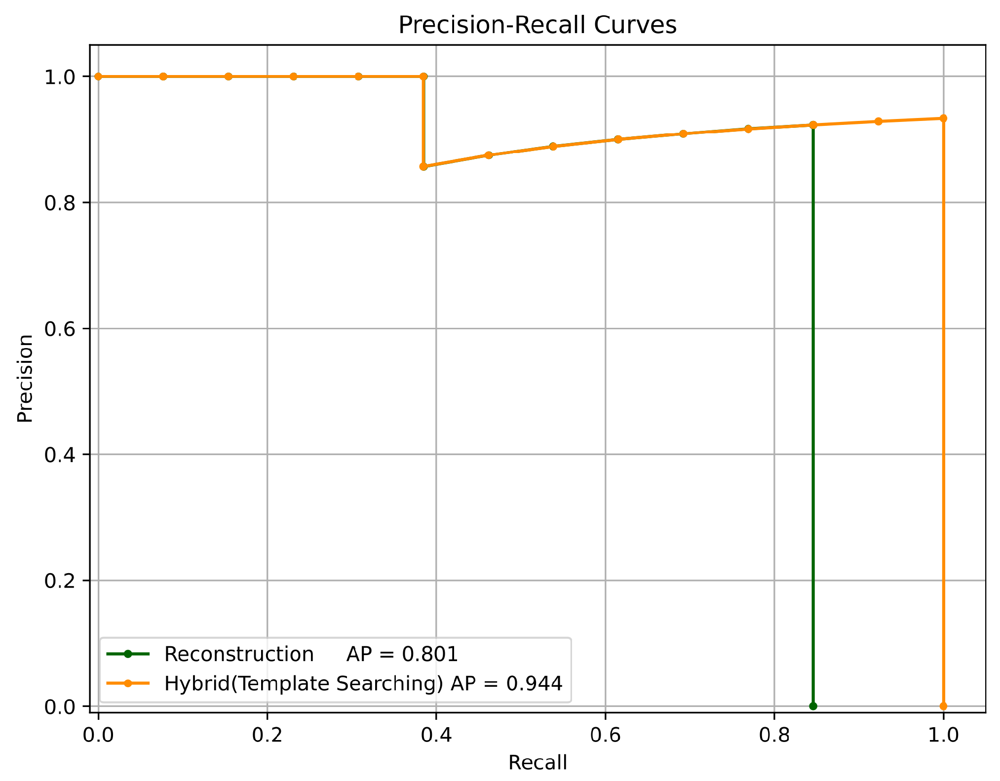
Precision–recall curves of two template generation approaches. The reconstruction approach achieved an AP of 0.801, while the proposed searching method reached an AP of 0.944.
Figure 26.
Precision–recall curves of two template generation approaches. The reconstruction approach achieved an AP of 0.801, while the proposed searching method reached an AP of 0.944.
Figure 27.
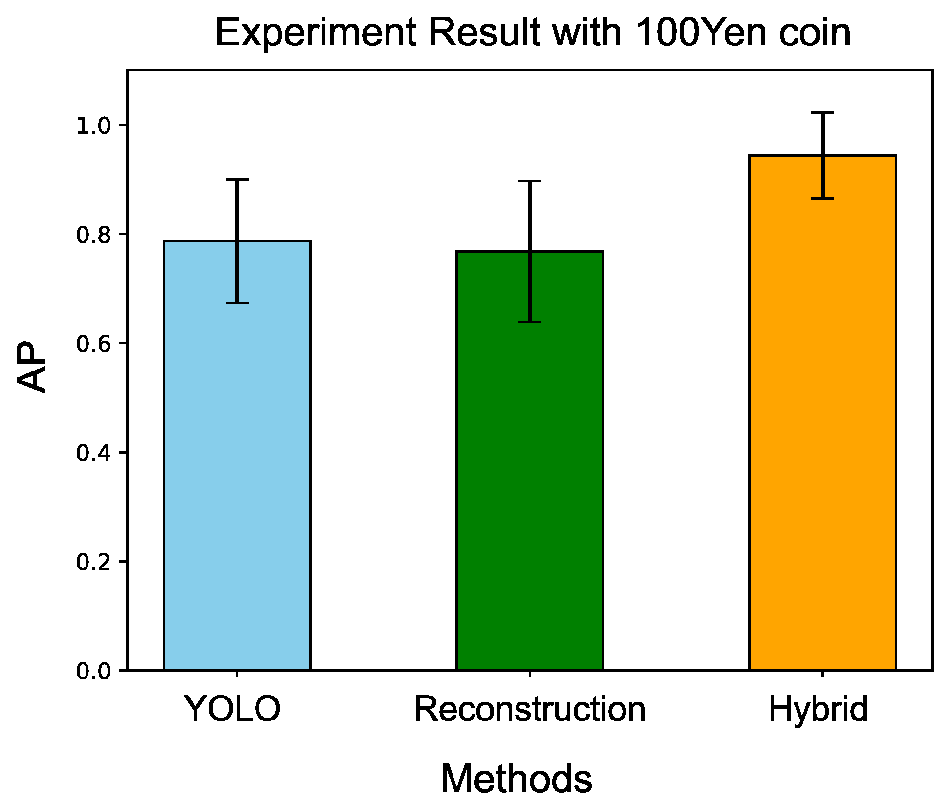
Comparison with three different methods. Our proposed hybrid method demonstrates the best performance among the compared methods.
Figure 27.
Comparison with three different methods. Our proposed hybrid method demonstrates the best performance among the compared methods.
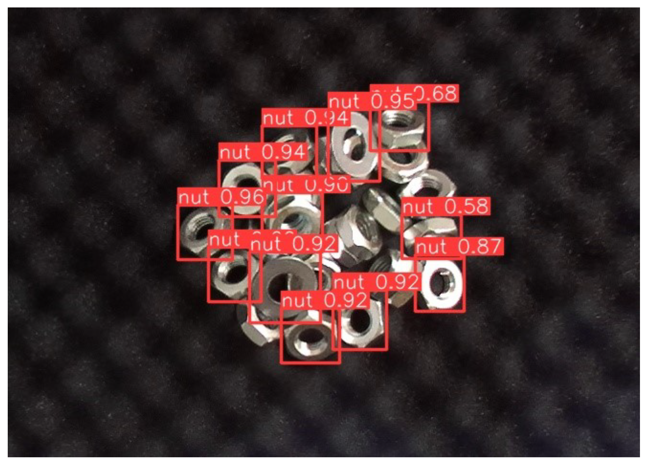
Figure 28.
YOLO’s detection result with the washer. The washers achieved confidence scores exceeding 0.90, which were even higher than those for the nuts.
Figure 28.
YOLO’s detection result with the washer. The washers achieved confidence scores exceeding 0.90, which were even higher than those for the nuts.
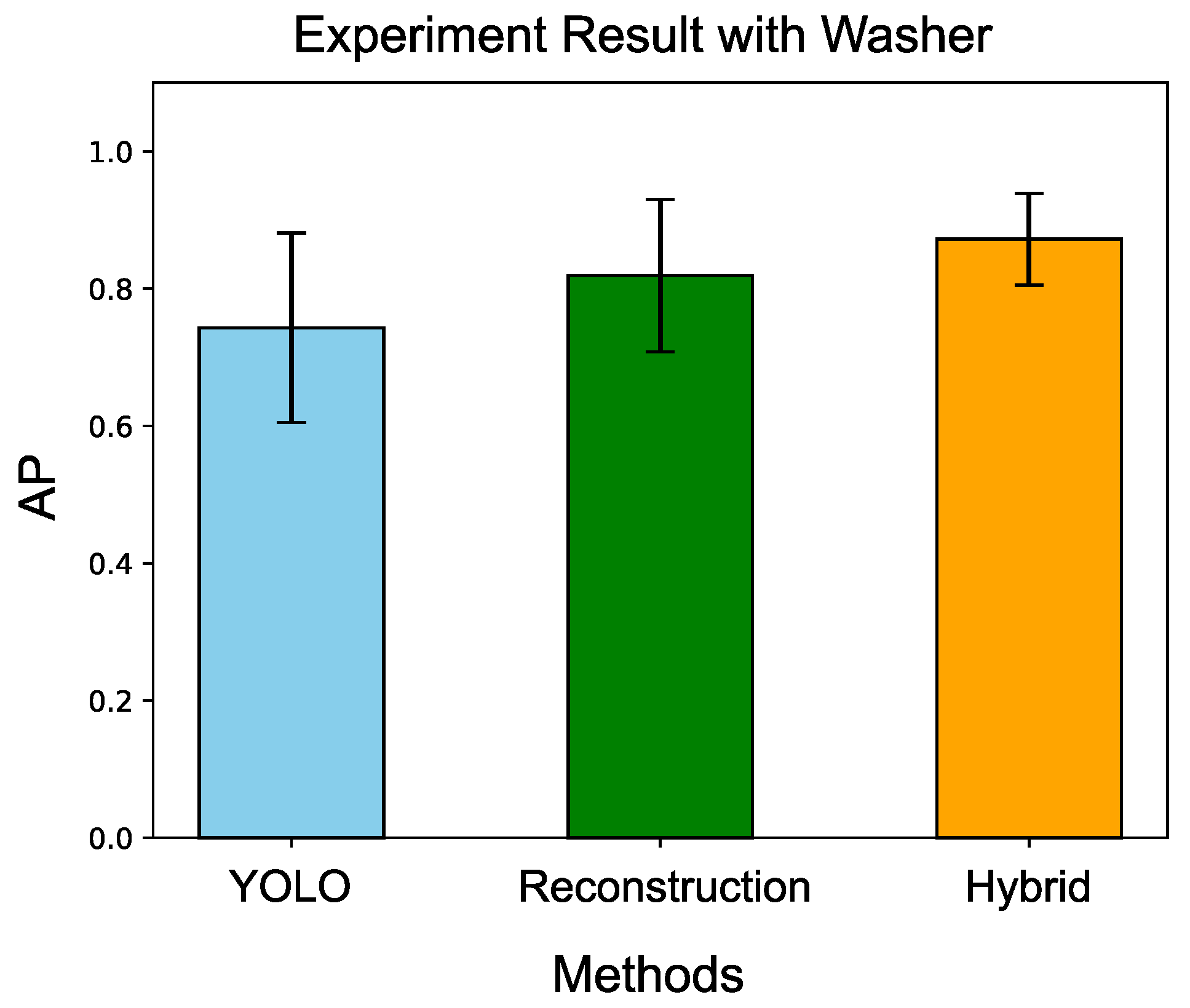
Figure 29.
Comparison with three different methods. Our proposed hybrid method demonstrates the best performance among the compared methods.
Figure 29.
Comparison with three different methods. Our proposed hybrid method demonstrates the best performance among the compared methods.
Figure 30.
Matching performance improvement after additional learning.
Figure 30.
Matching performance improvement after additional learning.
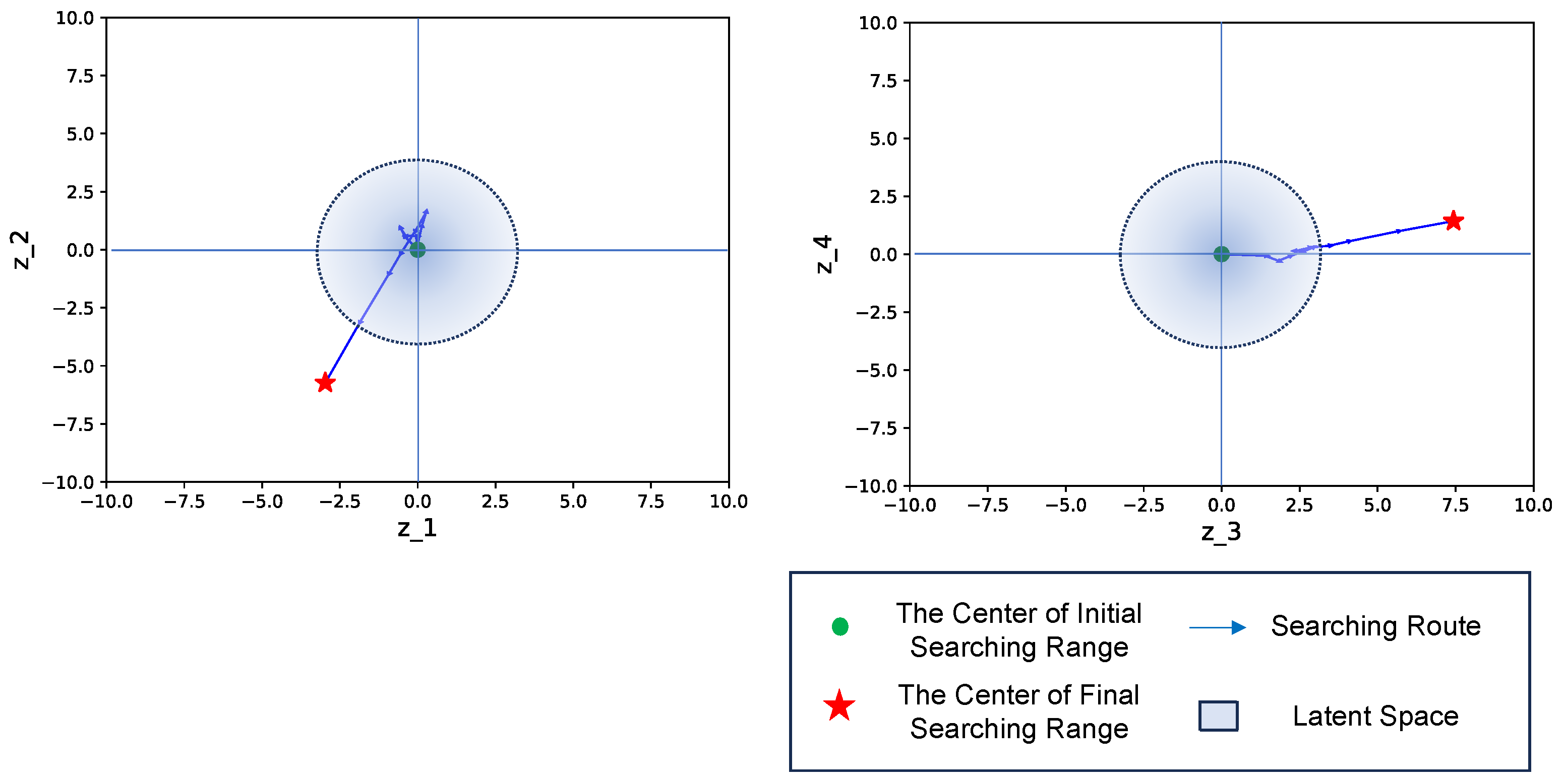
Figure 31.
The searching process before additional learning. An untrained situation resulted in the expected latent feature outside the trained latent space, leading to the generation of an unexpected template.
Figure 31.
The searching process before additional learning. An untrained situation resulted in the expected latent feature outside the trained latent space, leading to the generation of an unexpected template.
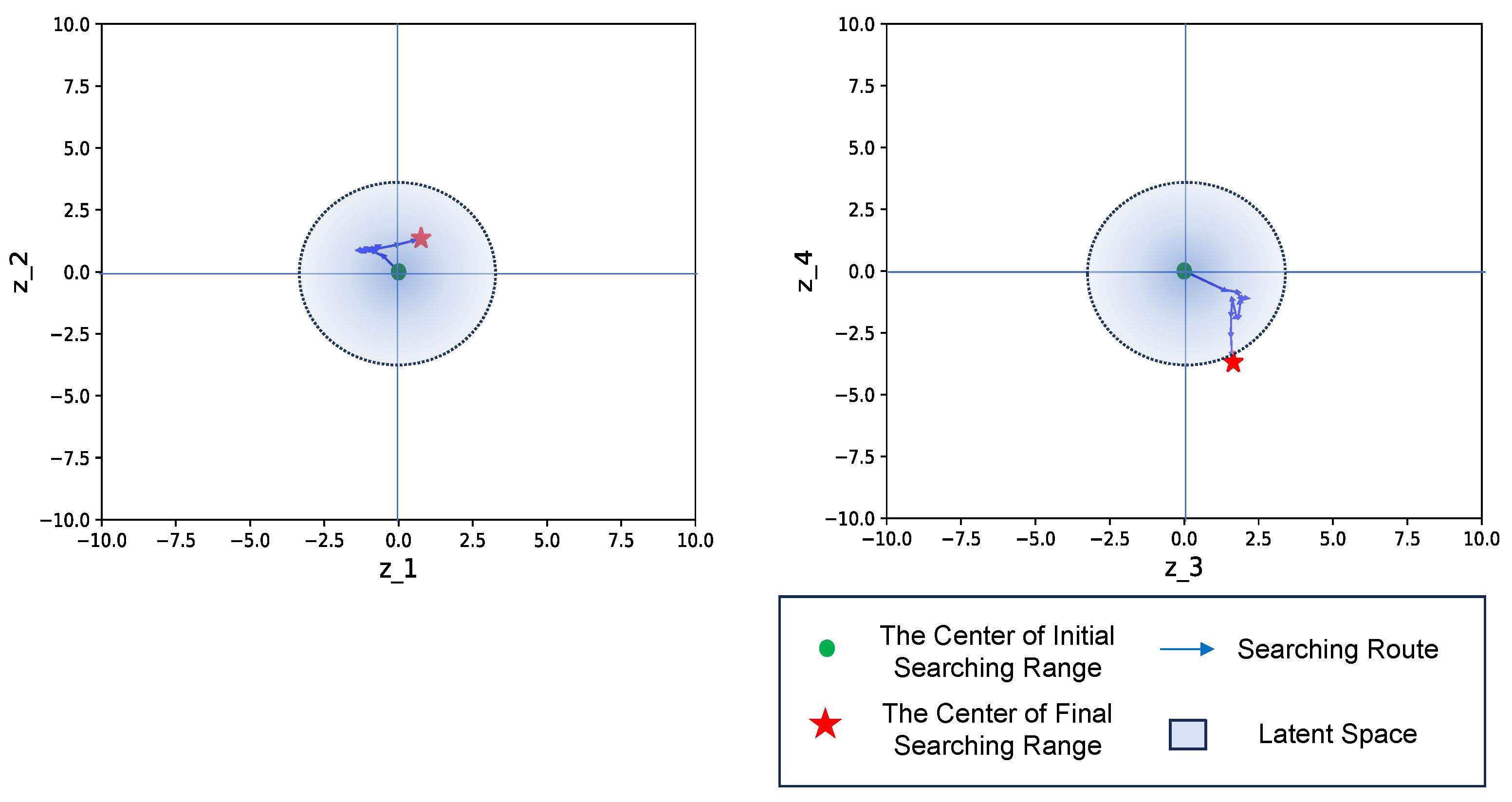
Figure 32.
The searching process after additional learning. After incorporating the annotated result, the search trajectory of the latent feature shifted closer to the retrained latent space. Consequently, the generated template exhibited improved matching performance.
Figure 32.
The searching process after additional learning. After incorporating the annotated result, the search trajectory of the latent feature shifted closer to the retrained latent space. Consequently, the generated template exhibited improved matching performance.
Figure 33.
Templates and their latent vectors generated by various approach. Based on YOLO’s results, corresponding templates were generated by template searching and the VAE reconstruction approaches. The results indicate that both the input factors and their combinations are critical.
Figure 33.
Templates and their latent vectors generated by various approach. Based on YOLO’s results, corresponding templates were generated by template searching and the VAE reconstruction approaches. The results indicate that both the input factors and their combinations are critical.
Table 1.
Template update time consumption for each strategy.
Table 1.
Template update time consumption for each strategy.
| Strategy | Time (second) |
|---|
| 150 templates | |
| 300 templates | |
| 600 templates | |
| 1500 templates | |
| Ours | |
Table 2.
Experiment results for different object’s poses using our proposed method.
Table 2.
Experiment results for different object’s poses using our proposed method.
| Trial | Success (%) | % Cleared | PPH |
|---|
| 1 | 100 | 100 | 220 |
| 2 | 100 | 100 | 223 |
| 3 | 100 | 100 | 221 |
| 4 | 100 | 100 | 224 |
| 5 | 100 | 100 | 224 |
Table 3.
Experiment results by different strategies.
Table 3.
Experiment results by different strategies.
| Strategy | Success (%) | % Cleared | PPH |
|---|
| 150 Templates | 100 | 99.2 | 238 |
| 300 Templates | 100 | 100 | 239 |
| 600 Templates | 100 | 100 | 219 |
| 1500 Templates | 100 | 100 | 209 |
| Ours | 100 | 100 | 222 |
Table 4.
Experiment results for varying background appearances by proposed method.
Table 4.
Experiment results for varying background appearances by proposed method.
| Trial | Success (%) | % Cleared | PPH |
|---|
| 1 | 92.8 | 100 | 206 |
| 2 | 90.9 | 100 | 204 |
| 3 | 92.6 | 100 | 207 |
| 4 | 90.3 | 100 | 211 |
| 5 | 90.0 | 100 | 208 |
Table 5.
Comparison with different strategies in varying background appearances condition.
Table 5.
Comparison with different strategies in varying background appearances condition.
| Strategy | Success (%) | % Cleared | PPH |
|---|
| 150 Templates | 92.7 | 44.8 | 203 |
| 300 Templates | 88.9 | 45.0 | 194 |
| 600 Templates | 89.5 | 98.0 | 180 |
| 1500 Templates | 92.8 | 100 | 147 |
| Ours | 91.3 | 100 | 207 |
Table 6.
Experiment results for additional lighting source.
Table 6.
Experiment results for additional lighting source.
| Trial | Success (%) | % Cleared | PPH |
|---|
| 1 | 92.6 | 100 | 213 |
| 2 | 92.6 | 100 | 211 |
| 3 | 89.6 | 100 | 199 |
| 4 | 90.3 | 100 | 206 |
| 5 | 93.3 | 100 | 228 |
Table 7.
Experiment results by different strategies in additional lighting source condition.
Table 7.
Experiment results by different strategies in additional lighting source condition.
| Strategy | Success (%) | % Cleared | PPH |
|---|
| 150 Templates | 80.1 | 32.8 | 171 |
| 300 Templates | 80.4 | 37.0 | 177 |
| 600 Templates | 84.4 | 80.0 | 172 |
| 1500 Templates | 90.9 | 100.0 | 142 |
| Ours | 91.7 | 100.0 | 211 |
Table 8.
Experiment results with 100-yen Coin.
Table 8.
Experiment results with 100-yen Coin.
| Trial | | |
|---|
| 1 | 0.890 | 1.000 |
| 2 | 0.748 | 0.917 |
| 3 | 0.919 | 1.000 |
| 4 | 0.807 | 0.743 |
| 5 | 0.878 | 0.878 |
| 6 | 0.762 | 0.944 |
| 7 | 0.629 | 0.944 |
| 8 | 0.620 | 1.000 |
| 9 | 0.701 | 1.000 |
| 10 | 0.911 | 0.983 |
Table 9.
Experiment results with different template generation approaches.
Table 9.
Experiment results with different template generation approaches.
| Trial | | |
|---|
| 1 | 0.900 | 1.000 |
| 2 | 0.497 | 0.917 |
| 3 | 0.827 | 1.000 |
| 4 | 0.666 | 0.743 |
| 5 | 0.680 | 0.878 |
| 6 | 0.747 | 0.944 |
| 7 | 0.801 | 0.944 |
| 8 | 0.889 | 1.000 |
| 9 | 0.762 | 1.000 |
| 10 | 0.911 | 0.983 |
Table 10.
Experiment results with washer by three different approaches.
Table 10.
Experiment results with washer by three different approaches.
| Trial | | | |
|---|
| 1 | 0.854 | 0.771 | 0.854 |
| 2 | 0.568 | 0.766 | 0.766 |
| 3 | 0.604 | 0.861 | 0.849 |
| 4 | 0.662 | 0.831 | 0.831 |
| 5 | 0.869 | 0.935 | 0.935 |
| 6 | 0.786 | 0.935 | 0.935 |
| 7 | 0.895 | 0.589 | 0.795 |
| 8 | 0.536 | 0.889 | 0.918 |
| 9 | 0.778 | 0.900 | 0.860 |
| 10 | 0.877 | 0.711 | 0.977 |


