

A Detection Transformer-Based Intelligent Identification Method for Multiple Types of Road Traffic Safety Facilities

Abstract
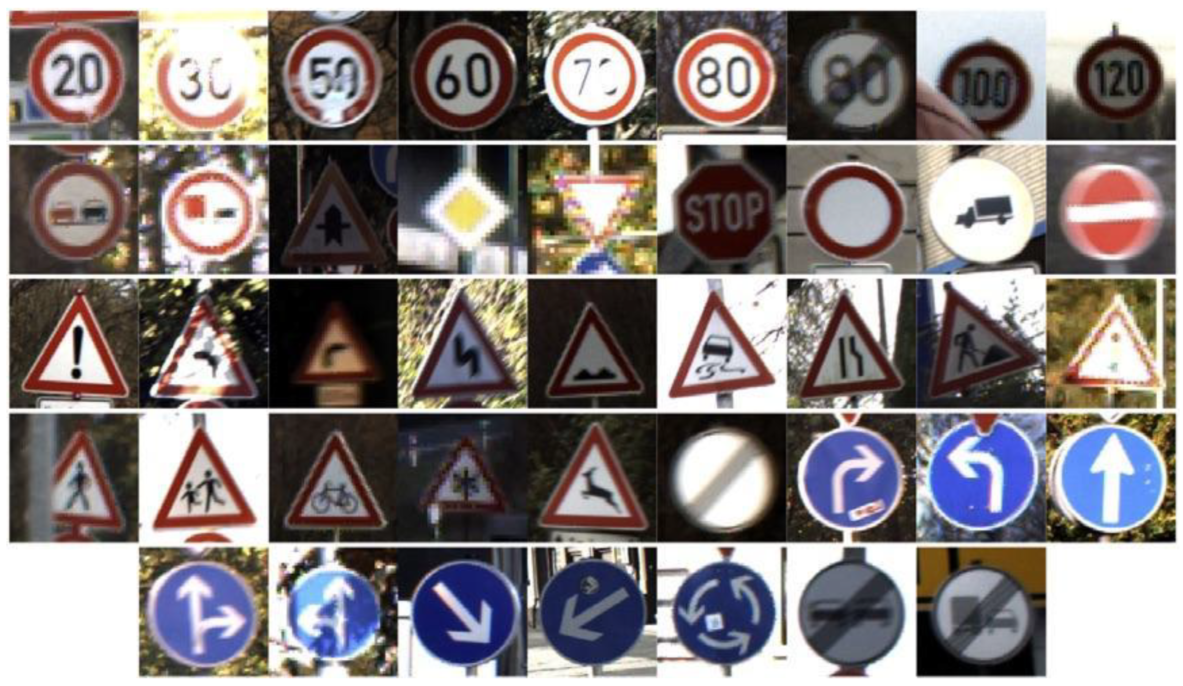
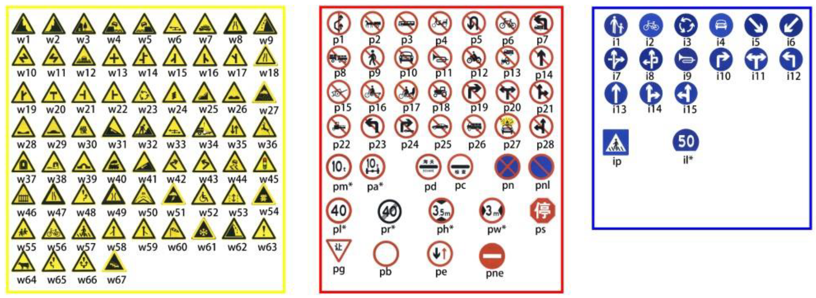
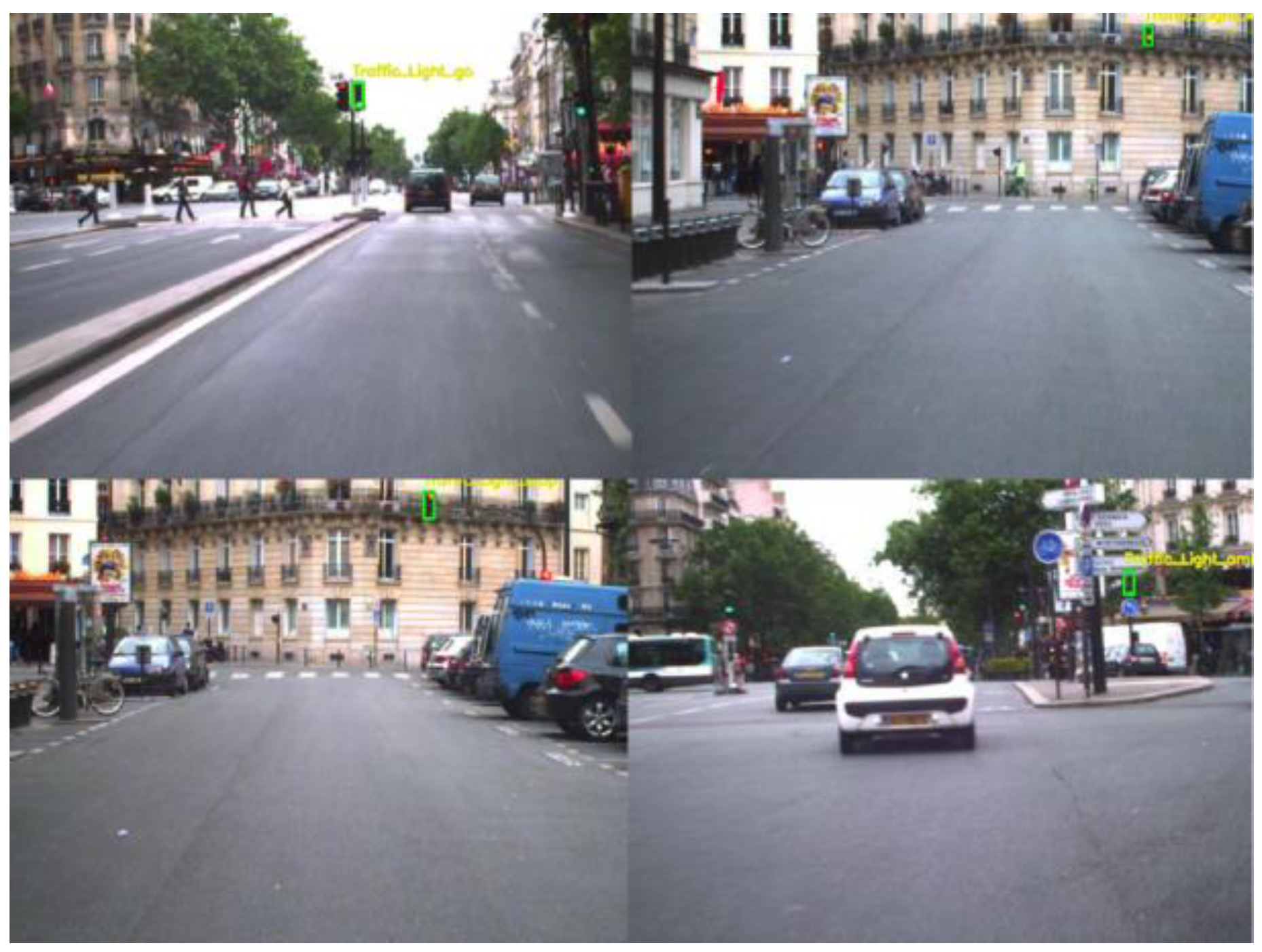
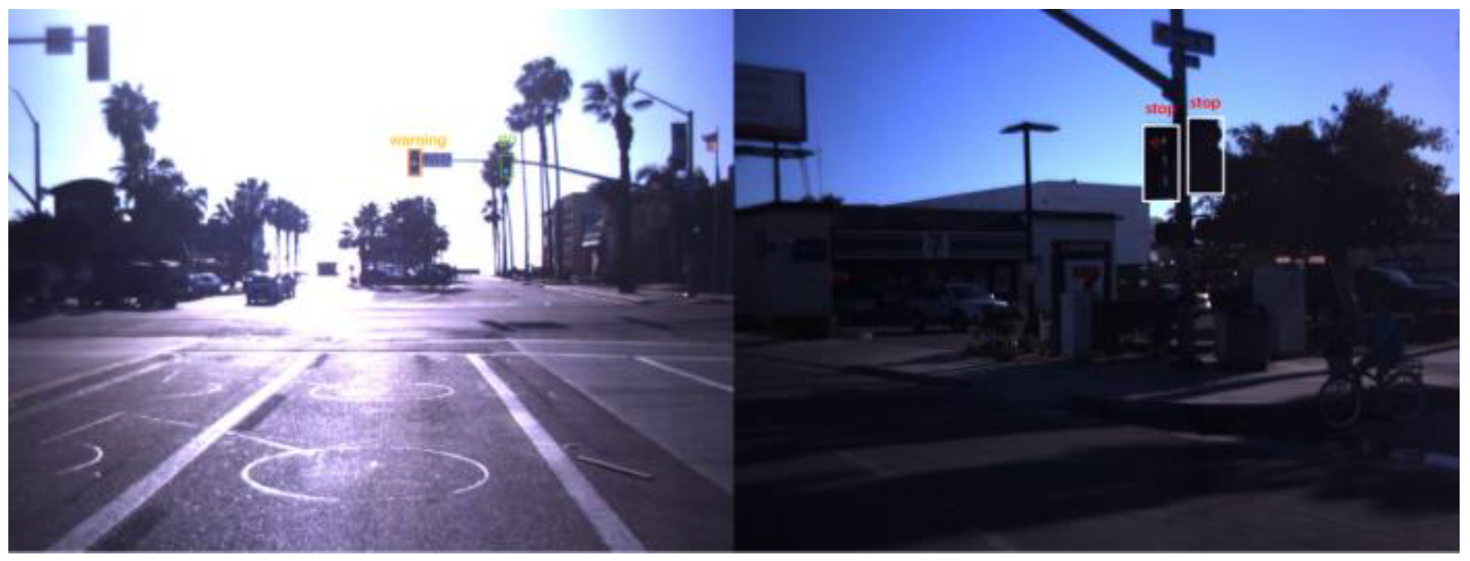
1. Introduction
2. Methodology
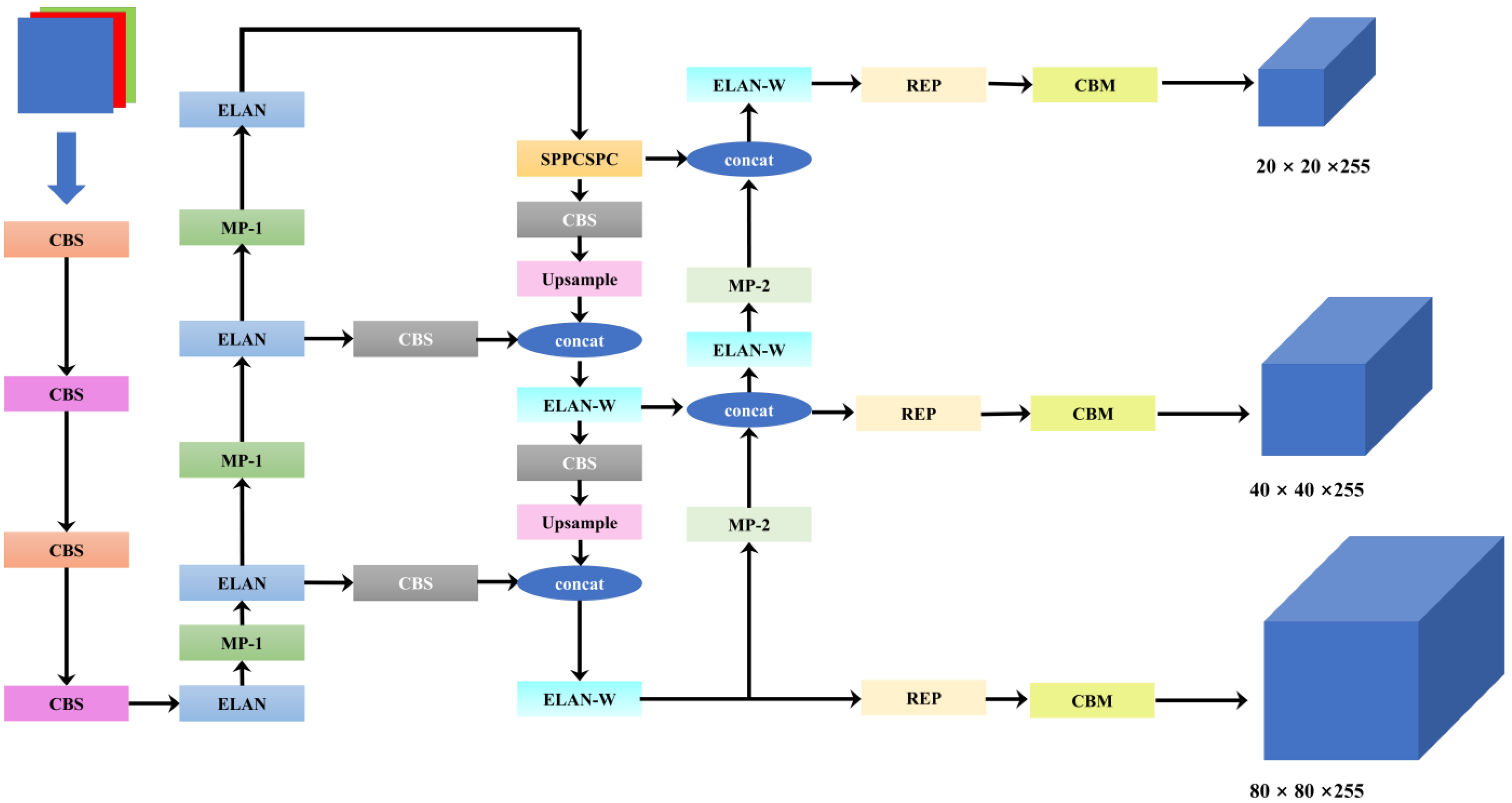
2.1. YOLOv7
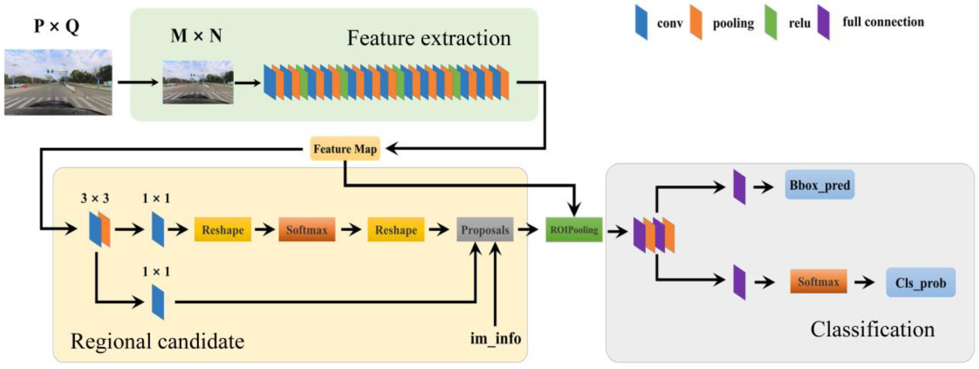
2.2. Faster-RCNN
2.3. DN-DETR and DINO
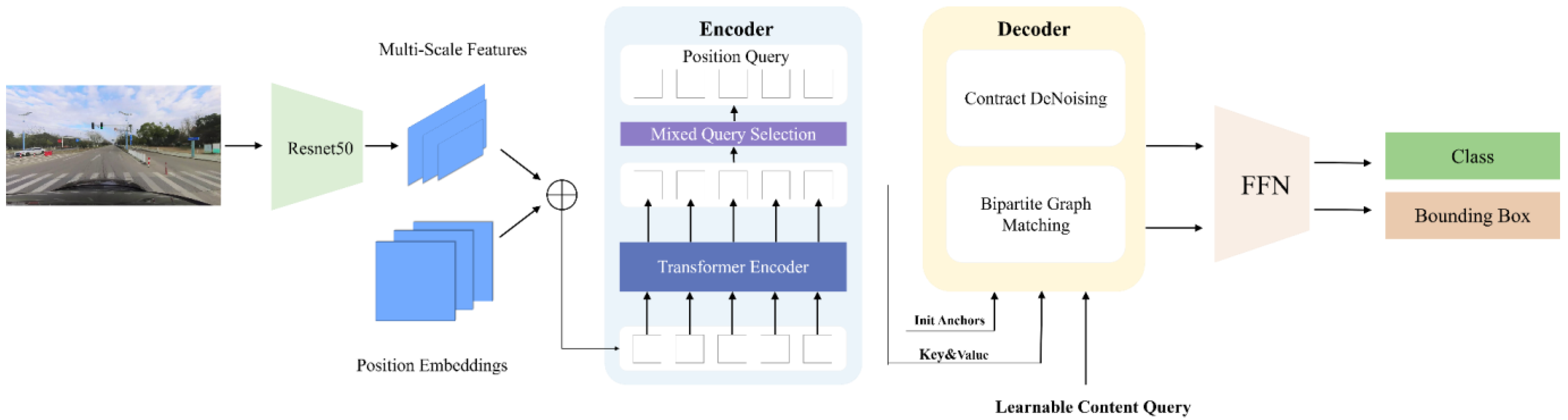
2.3.1. Introduction of the DINO Model
2.3.2. Contrastive DeNoising Approach
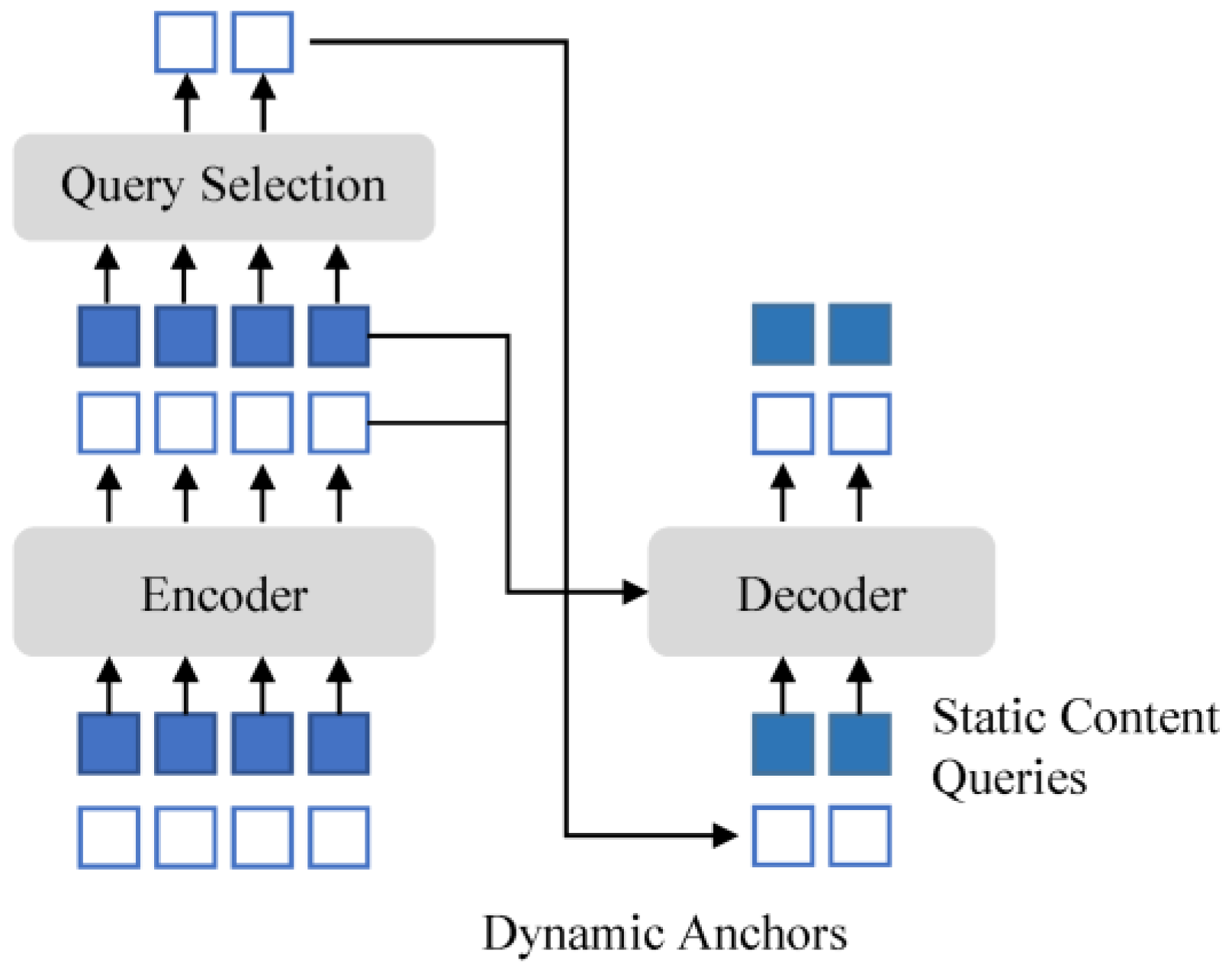
2.3.3. Mixed Query Selection
2.3.4. Look-Forward Twice Mechanism
3. Experiment
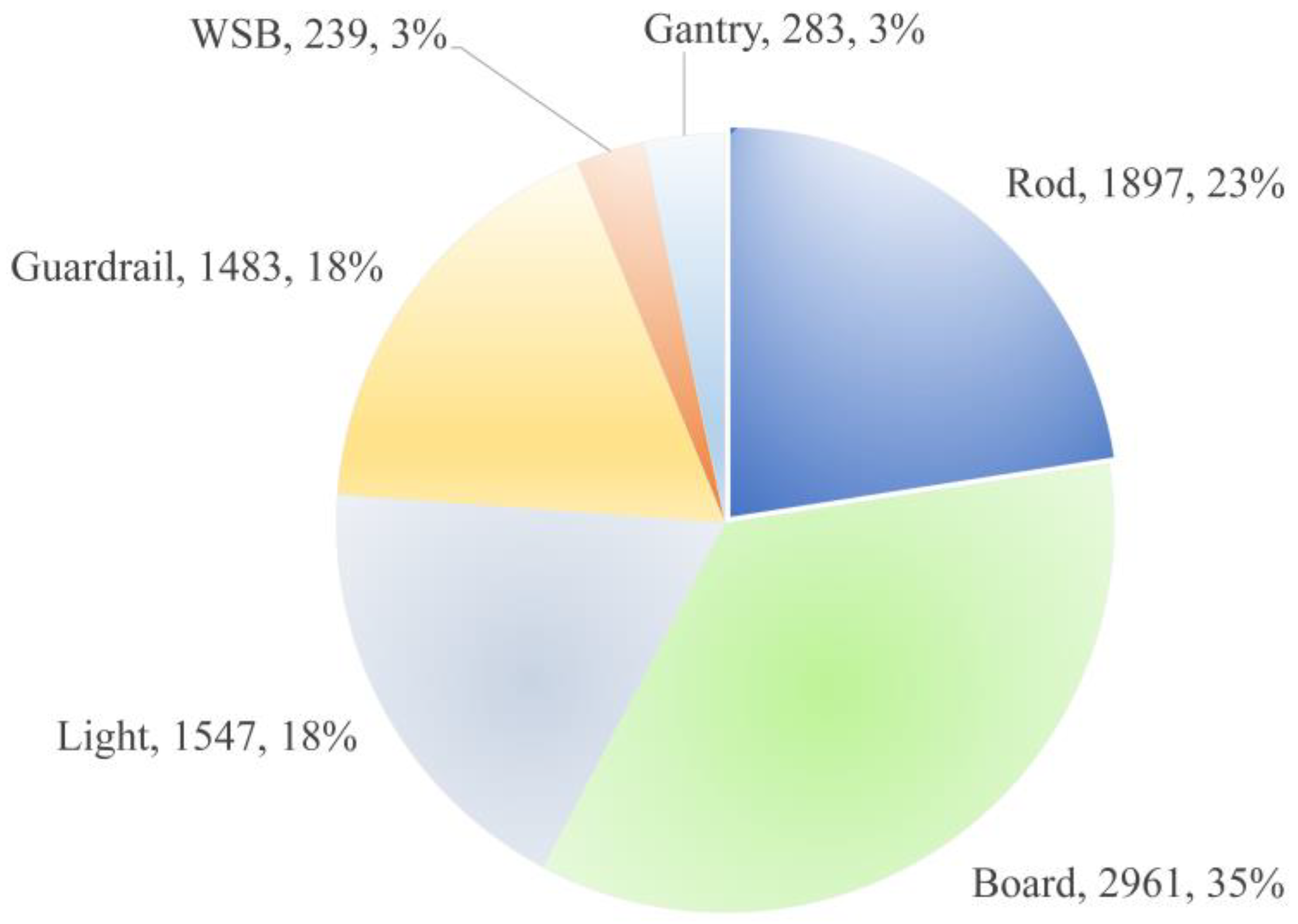
3.1. TSF-CQU Dataset
3.2. Evaluation Metrics
3.3. Experimental Setup and Model Training
3.4. Ablation Experiment of DINO Components
4. Results and Discussion
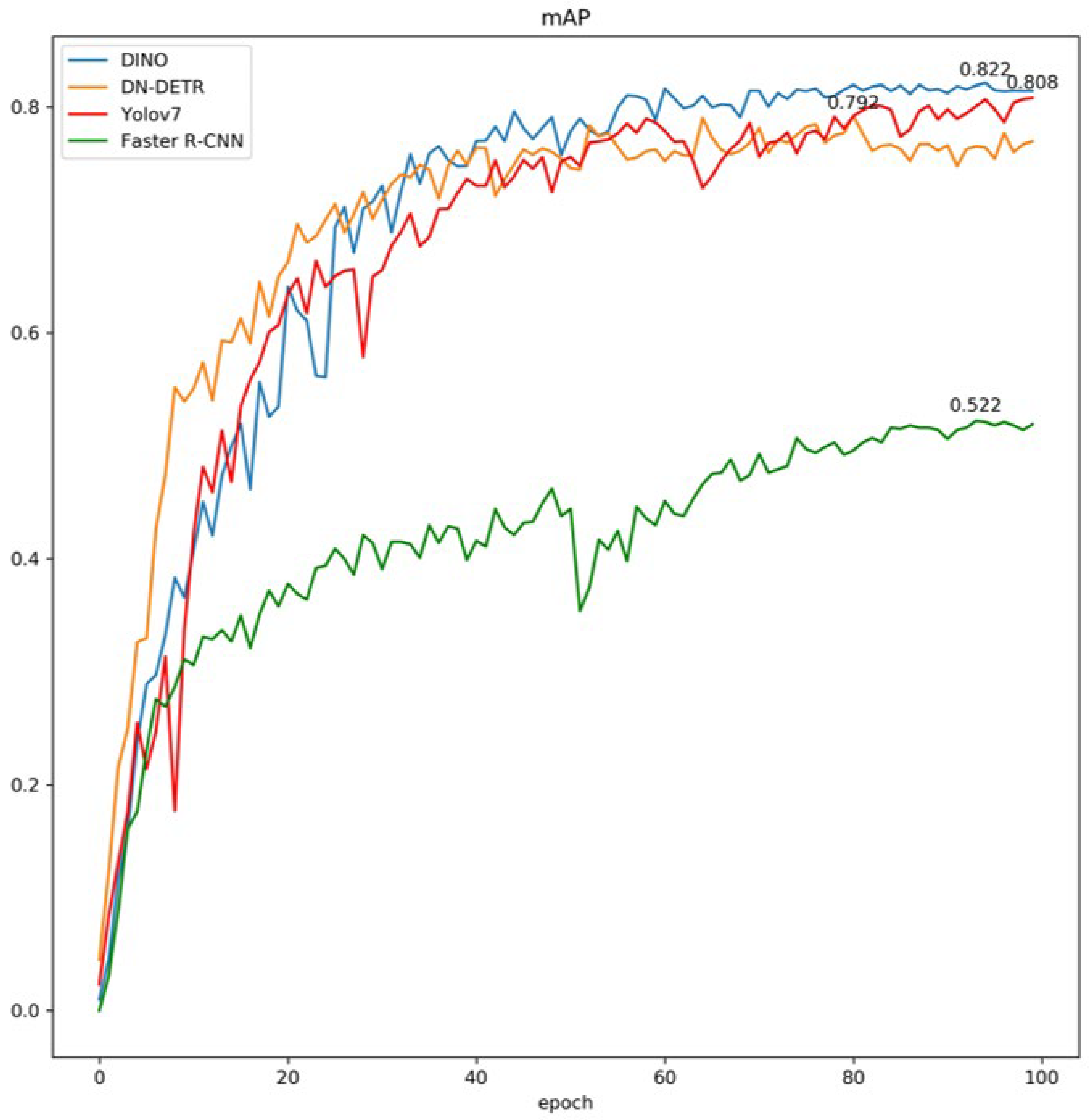
4.1. The Training Process of DINO
4.2. Comparison of Models
4.2.1. Training Results
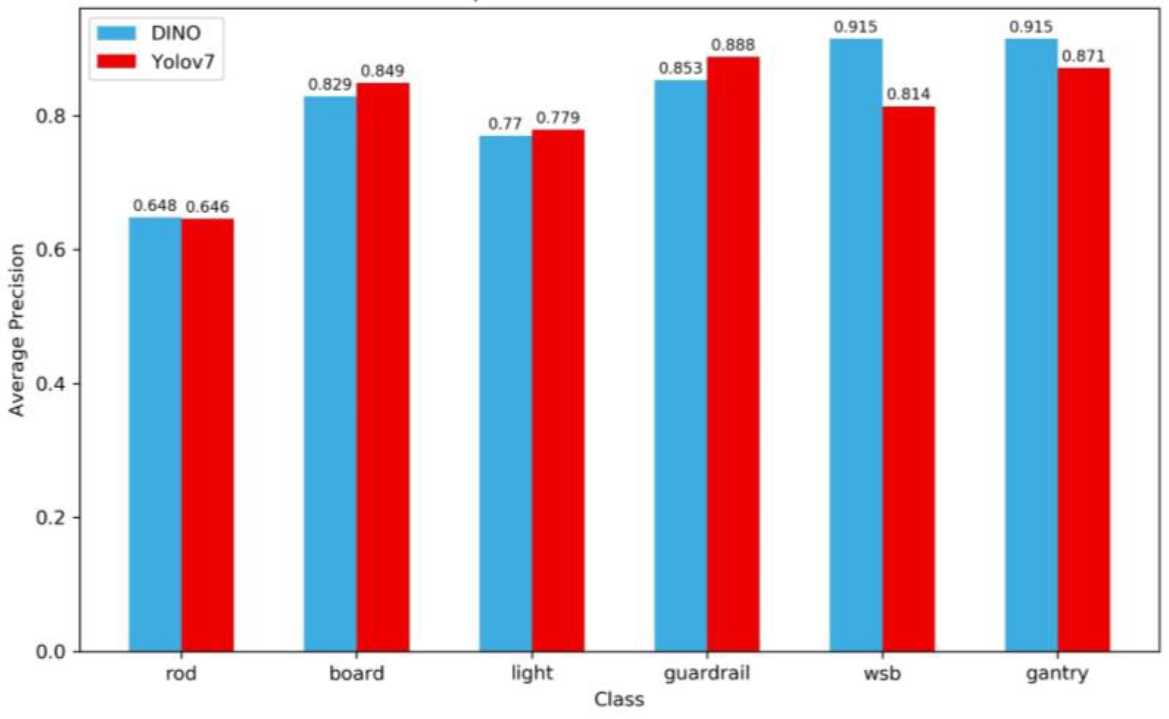
4.2.2. Comparison of Detection Precision of DINO and Yolov7 for Each Category
4.3. Ablation Experiment Results
4.3.1. Comparison of the Overall Training Results
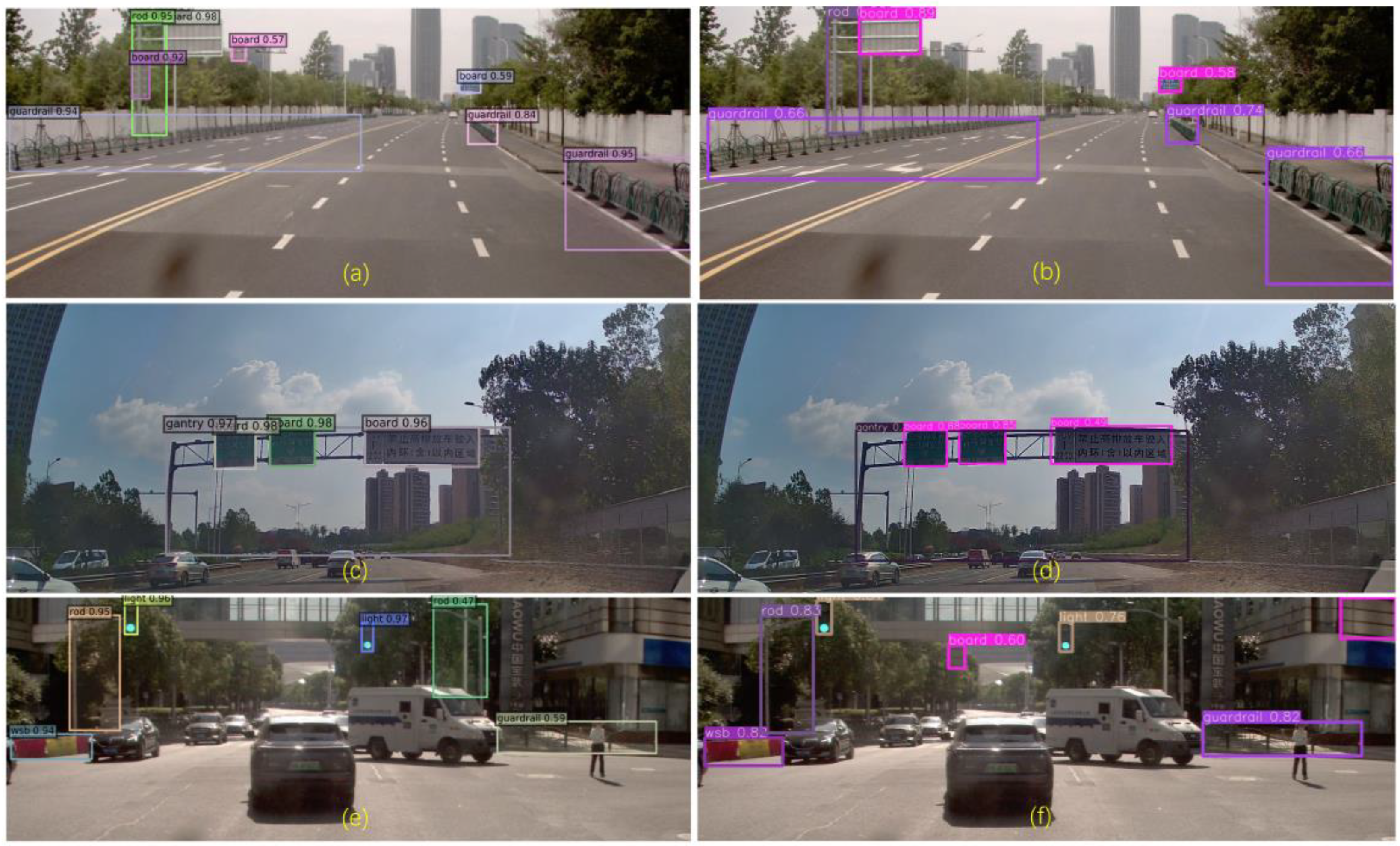
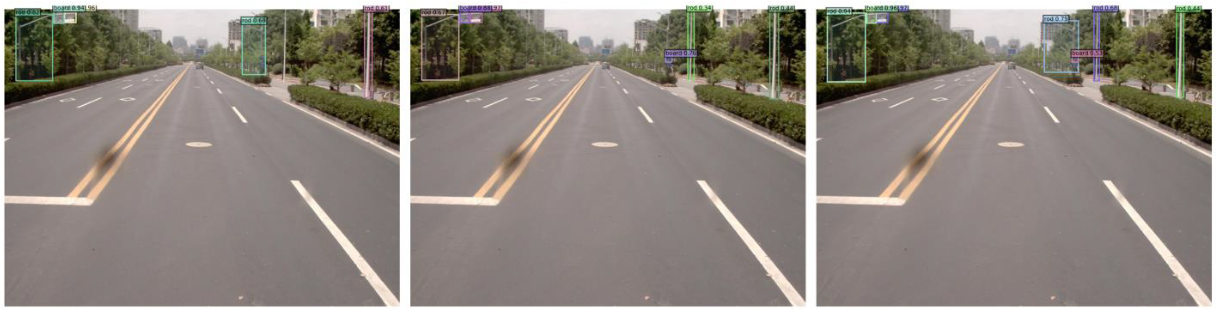
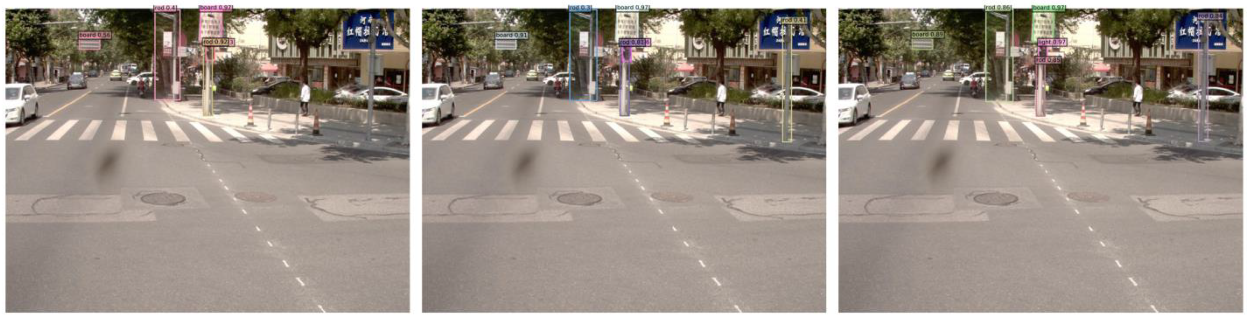
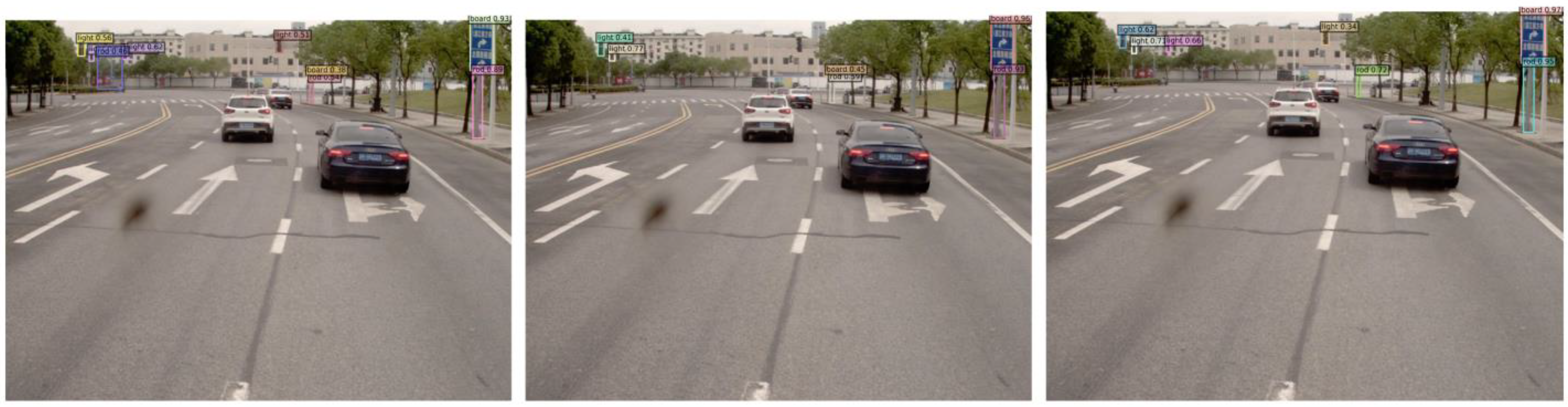
4.3.2. Case Analysis
4.4. Efficiency Analysis of the DINO Model for TSF Detection
5. Conclusions
- Traffic safety facilities were included in the study as intelligent recognition objects from an asset management perspective, and a target detection dataset called TSF-CQU was constructed, including six types of TSFs, 1437 images, and 8420 instances.
- Using the DINO model, accurate recognition of TSFs was successfully achieved with an mAP of 82.2%, but the advantage over Yolov7 is not significant.
- The DINO model rarely makes misjudgments, but there is a certain degree of missed detection, mainly including traffic rods.
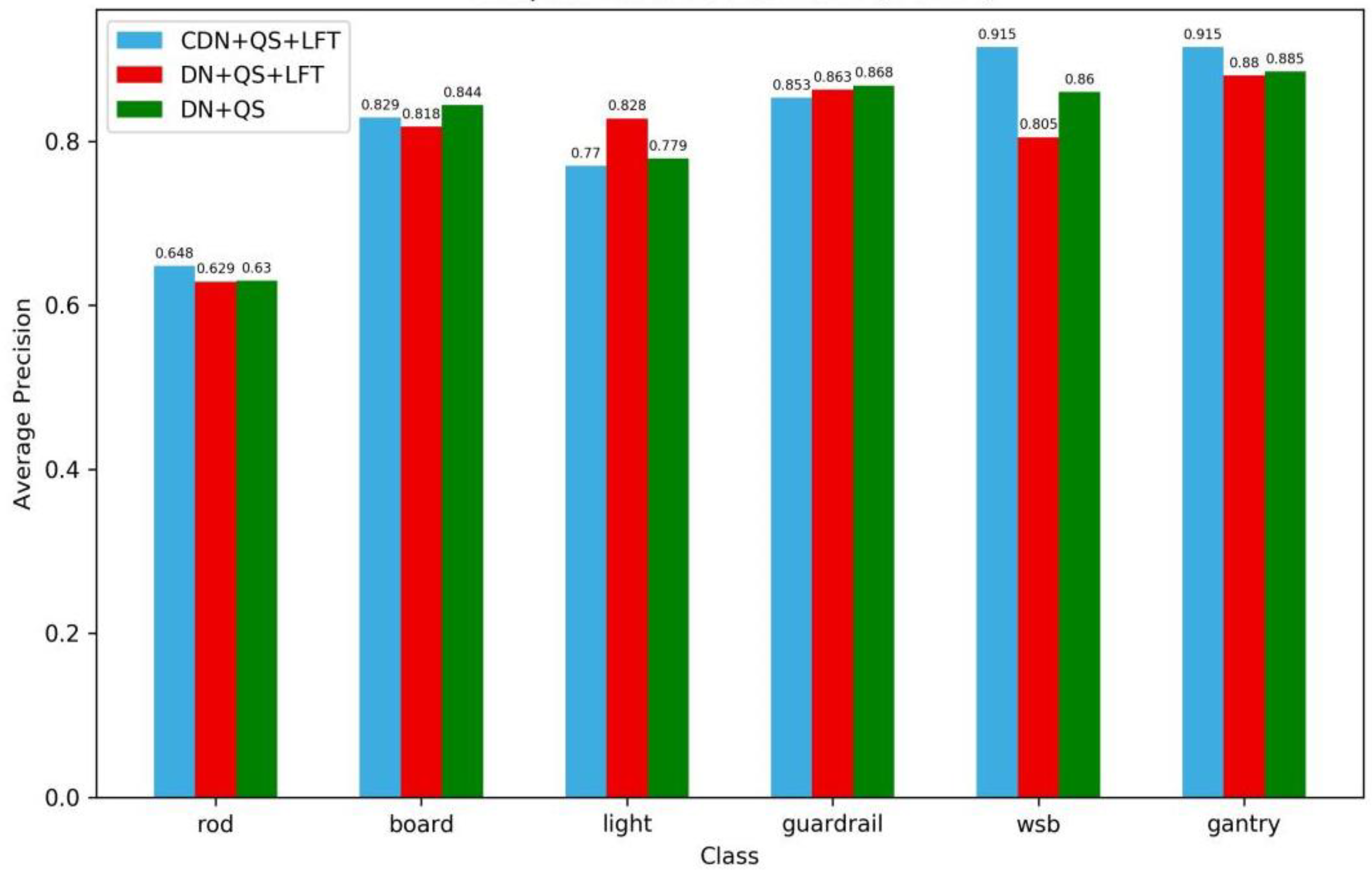
- CDN is not conducive to the detection of lights, and LFT is counterproductive for the detection of boards. DINO provides the most significant improvement in the detection of continuous-type large targets, such as WSBs and gantries, in comparison to DQ and DQL.
Author Contributions
Funding
Institutional Review Board Statement
Informed Consent Statement
Data Availability Statement
Conflicts of Interest
References
- GB50688-2011(2019); Code for the Design of Urban Road Traffic Facility. Ministry of Housing and Urban-Rural Development of the People’s Republic of China: Beijing, China, 2019.
- Min, W.; Liu, R.; He, D.; Han, Q.; Wei, Q.; Wang, Q. Traffic Sign Recognition Based on Semantic Scene Understanding and Structural Traffic Sign Location. IEEE Trans. Intell. Transp. Syst. 2022, 23, 15794–15807. [Google Scholar] [CrossRef]
- Zhu, Y.; Yan, W.Q. Traffic sign recognition based on deep learning. Multimedia Tools Appl. 2022, 81, 17779–17791. [Google Scholar] [CrossRef]
- Wang, Z.; Wang, J.; Li, Y.; Wang, S. Traffic Sign Recognition with Lightweight Two-Stage Model in Complex Scenes. IEEE Trans. Intell. Transp. Syst. 2022, 23, 1121–1131. [Google Scholar] [CrossRef]
- Chen, R.; Hei, L.; Lai, Y. Image Recognition and Safety Risk Assessment of Traffic Sign Based on Deep Convolution Neural Network. IEEE Access 2020, 8, 201799–201805. [Google Scholar] [CrossRef]
- Almeida, T.; Macedo, H.; Matos, L.; Prado, B.; Bispo, K. Frequency Maps as Expert Instructions to lessen Data Dependency on Real-time Traffic Light Recognition. In Proceedings of the 2020 International Conference on Computational Science and Computational Intelligence (CSCI), Las Vegas, NV, USA, 16–18 December 2020; pp. 1463–1468. [Google Scholar] [CrossRef]
- De Charette, R.; Nashashibi, F. Traffic light recognition using image processing compared to learning processes. In Proceedings of the 2009 IEEE/RSJ International Conference on Intelligent Robots and Systems, St. Louis, MO, USA, 11–15 October 2009; IEEE: New York, NY, USA, 2009; pp. 333–338. [Google Scholar]
- Johner, F.M.; Wassner, J. Efficient evolutionary architecture search for CNN optimization on GTSRB. In Proceedings of the 2019 18th IEEE International Conference On Machine Learning, and Applications (ICMLA), Boca Raton, FL, USA, 16–19 December 2019; IEEE: New York, NY, USA, 2019; pp. 56–61. [Google Scholar]
- Zhu, Z.; Liang, D.; Zhang, S.; Huang, X.; Li, B.; Hu, S. Traffic-sign detection and classification in the wild. In Proceedings of the IEEE Conference on Computer Vision and Pattern Recognition, Las Vegas, NV, USA, 27–30 June 2016; pp. 2110–2118. [Google Scholar]
- Behrendt, K.; Novak, L.; Botros, R. A deep learning approach to traffic lights: Detection, tracking, and classification. In Proceedings of the 2017 IEEE International Conference on Robotics and Automation (ICRA), Singapore, 29 May–3 June 2017; IEEE: New York, NY, USA, 2017; pp. 1370–1377. [Google Scholar]
- Philipsen, M.P.; Jensen, M.B.; Mogelmose, A.; Moeslund, T.B.; Trivedi, M.M. Traffic light detection: A learning algorithm and evaluations on challenging dataset. In Proceedings of the 2015 IEEE 18th International Conference on Intelligent Transportation Systems, Gran Canaria, Spain, 15–18 September 2015; IEEE: New York, NY, USA, 2015; pp. 2341–2345. [Google Scholar]
- Arcos-García, Á.; Alvarez-Garcia, J.A.; Soria-Morillo, L.M. Deep neural network for traffic sign recognition systems: An analysis of spatial transformers and stochastic optimization methods. Neural Netw. 2018, 99, 158–165. [Google Scholar] [CrossRef]
- Chen, J.; Jia, K.; Chen, W.; Lv, Z.; Zhang, R. A real-time and high-precision method for small traffic-signs recognition. Neural Comput. Appl. 2022, 34, 2233–2245. [Google Scholar] [CrossRef]
- Wang, Q.; Zhang, Q.; Liang, X.; Wang, Y.; Zhou, C.; Mikulovich, V.I. Traffic lights detection and recognition method based on the improved YOLOv4 algorithm. Sensors 2022, 22, 200. [Google Scholar] [CrossRef]
- Wang, L.; Zhou, K.; Chu, A.; Wang, G.; Wang, L. An Improved Light-Weight Traffic Sign Recognition Algorithm Based on YOLOv4-Tiny. IEEE Access 2021, 9, 124963–124971. [Google Scholar] [CrossRef]
- Pon, A.; Adrienko, O.; Harakeh, A.; Waslander, S.L. A hierarchical deep architecture and mini-batch selection method for joint traffic sign and light detection. In Proceedings of the 2018 15th Conference on Computer and Robot Vision (CRV), Toronto, ON, Canada, 9–11 May 2018; IEEE: New York, NY, USA, 2018; pp. 102–109. [Google Scholar]
- Ning, Z.; Wang, H.; Li, S.; Xu, Z. YOLOv7-RDD: A Lightweight Efficient Pavement Distress Detection Model. IEEE Trans. Intell. Transp. Syst. 2021, 1–9. [Google Scholar] [CrossRef]
- Ha, T.T.; Chaisomphob, T. Automated Localization and Classification of Expressway Pole-Like Road Facilities from Mobile Laser Scanning Data. Adv. Civ. Eng. 2020, 2020, 5016783. [Google Scholar] [CrossRef]
- Liu, Z.; Gu, X.; Yang, H.; Wang, L.; Chen, Y.; Wang, D. Novel YOLOv3 model with structure and hyperparameter optimization for detection of pavement concealed cracks in GPR images. IEEE Trans. Intell. Transp. Syst. 2022, 23, 22258–22268. [Google Scholar] [CrossRef]
- Wang, D.; Liu, Z.; Gu, X.; Wu, W.; Chen, Y.; Wang, L. Automatic detection of pothole distress in asphalt pavement using improved convolutional neural networks. Remote Sens. 2022, 14, 3892. [Google Scholar] [CrossRef]
- Liu, Z.; Gu, X.; Chen, J.; Wang, D.; Chen, Y.; Wang, L. Automatic recognition of pavement cracks from combined GPR B-scan and C-scan images using multiscale feature fusion deep neural networks. Autom. Constr. 2023, 146, 104698. [Google Scholar] [CrossRef]
- Girshick, R.; Donahue, J.; Darrell, T.; Malik, J. Rich feature hierarchies for accurate object detection and semantic segmentation. In Proceedings of the IEEE Conference on Computer Vision and Pattern Recognition, Columbus, OH, USA, 23–28 June 2014; pp. 580–587. [Google Scholar] [CrossRef]
- Jiang, P.; Ergu, D.; Liu, F.; Cai, Y.; Ma, B. A Review of Yolo algorithm developments. Procedia Comput. Sci. 2022, 199, 1066–1073. [Google Scholar] [CrossRef]
- Ren, S.; He, K.; Girshick, R.; Sun, J. Faster R-CNN: Towards Real-Time Object Detection with Region Proposal Networks. IEEE Trans. Pattern Anal. Mach. Intell. 2017, 39, 1137–1149. [Google Scholar] [CrossRef] [PubMed]
- Zhu, J.; Zhong, J.; Ma, T.; Huang, X.; Zhang, W.; Zhou, Y. Pavement distress detection using convolutional neural networks with images captured via UAV. Autom. Constr. 2022, 133, 103991. [Google Scholar] [CrossRef]
- Lei, X.; Liu, C.; Li, L.; Wang, G. Automated Pavement Distress Detection and Deterioration Analysis Using Street View Map. IEEE Access 2020, 8, 76163–76172. [Google Scholar] [CrossRef]
- Terven, J.; Córdova-Esparza, D.-M.; Romero-González, J.-A. A Comprehensive Review of YOLO Architectures in Computer Vision: From YOLOv1 to YOLOv8 and YOLO-NAS. Mach. Learn. Knowl. Extr. 2023, 5, 1680–1716. [Google Scholar] [CrossRef]
- Wang, C.Y.; Bochkovskiy, A.; Liao, H.Y.M. Yolov7: Trainable bag-of-freebies sets new state-of-the-art for real-time object detectors. arXiv 2022. [Google Scholar] [CrossRef]
- Rangari, A.P.; Chouthmol, A.R.; Kadadas, C.; Pal, P.; Singh, S.K. Deep Learning based smart traffic light system using Image Processing with YOLO v7. In Proceedings of the 2022 4th International Conference on Circuits, Control, Communication and Computing (I4C), Bangalore, India, 21–23 December 2022; pp. 129–132. [Google Scholar] [CrossRef]
- Chen, J.; Bai, S.; Wan, G.; Li, Y. Research on Yolov7-based defect detection method for automotive running lights. Syst. Sci. Control Eng. 2023, 11, 2185916. [Google Scholar] [CrossRef]
- Terven, J.R.; Cordova-Esparza, D.M. A Comprehensive Review of YOLO: From YOLOv1 and Beyond. 2023. Available online: http://arxiv.org/pdf/2304.00501v3 (accessed on 27 June 2023).
- Baghbanbashi, M.; Raji, M.; Ghavami, B. Quantizing Yolov7: A Comprehensive Study. In Proceedings of the 2023 28th International Computer Conference, Computer Society of Iran (CSICC), Tehran, Iran, 25–26 January 2023; pp. 1–5. [Google Scholar] [CrossRef]
- Carion, N.; Massa, F.; Synnaeve, G.; Usunier, N.; Kirillov, A.; Zagoruyko, S. End-to-end object detection with transformers. In Proceedings of the Computer Vision–ECCV 2020: 16th European Conference, Glasgow, UK, 23–28 August 2020; Proceedings, Part I 16. Springer International Publishing: Berlin/Heidelberg, Germany, 2020; pp. 213–229. [Google Scholar]
- Li, F.; Zhang, H.; Liu, S.; Guo, J.; Ni, L.M.; Zhang, L. Dn-detr: Accelerate detr training by introducing query denoising. In Proceedings of the IEEE/CVF Conference on Computer Vision and Pattern Recognition, New Orleans, LA, USA, 18–24 June 2022; pp. 13619–13627. [Google Scholar]
- Zhang, H.; Li, F.; Liu, S.; Zhang, L.; Su, H.; Zhu, J.; Ni, L.M.; Shum, H.Y. DINO: Detr with improved denoising anchor boxes for end-to-end object detection. arXiv 2022, arXiv:2203.03605. [Google Scholar]
- Lin, T.Y.; Dollár, P.; Girshick, R.; He, K.; Hariharan, B.; Belongie, S. Feature pyramid networks for object detection. In Proceedings of the IEEE Conference on Computer Vision and Pattern Recognition, Honolulu, HI, USA, 21–26 July 2017; pp. 2117–2125. [Google Scholar] [CrossRef]
- He, K.; Zhang, X.; Ren, S.; Sun, J. Deep residual learning for image recognition. In Proceedings of the IEEE Conference on Computer Vision and Pattern Recognition, Las Vegas, NV, USA, 27–30 June 2016; pp. 770–778. [Google Scholar] [CrossRef]
- Zhu, X.; Su, W.; Lu, L.; Li, B.; Wang, X.; Dai, J. Deformable DETR: Deformable transformers for end-to-end object detection. arXiv 2020, arXiv:2010.04159. [Google Scholar] [CrossRef]
- Bebis, G.; Georgiopoulos, M. Feed-forward neural networks. IEEE Potentials 1994, 13, 27–31. [Google Scholar] [CrossRef]
- Rezatofighi, H.; Tsoi, N.; Gwak, J.; Sadeghian, A.; Reid, I.; Savarese, S. Generalized intersection over union: A metric and a loss for bounding box regression. In Proceedings of the IEEE/CVF Conference on Computer Vision and Pattern Recognition, Long Beach, CA, USA, 16–17 June 2019; pp. 658–666. [Google Scholar] [CrossRef]
- Loshchilov, I.; Hutter, F. Fixing Weight Decay Regularization in Adam. arXiv 2017, arXiv:1711.05101. [Google Scholar] [CrossRef]
- Smith, L.N.; Topin, N. Super-convergence: Very fast training of neural networks using large learning rates. In Artificial Intelligence and Machine Learning for Multi-Domain Operations Applications; SPIE: Bellingham, WA, USA, 2019; Volume 11006, pp. 369–386. [Google Scholar] [CrossRef]
- Lin, T.; Goyal, P.; Girshick, R.; He, K.; Dollár, P. Focal loss for dense object detection. In Proceedings of the IEEE International Conference on Computer Vision, Venice, Italy, 22–29 October 2017; pp. 2980–2988. [Google Scholar] [CrossRef]


| NO. | Categories | Examples |
|---|---|---|
| 1 | Traffic rod (Rod) Note: Traffic warn information in Chinese. | 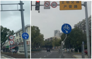 |
| 2 | Traffic sign (Board) Note: Traffic warn and guide information in Chinese are shown on the board. |  |
| 3 | Light | 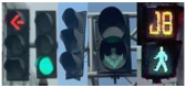 |
| 4 | Guardrail | 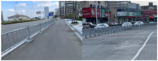 |
| 5 | Water surround barrier (WSB/wsb) |  |
| 6 | Gantry Note: Traffic guide information in Chinese are shown on the board. |  |
| Models | Params | GFLOPs | FPS | Training Time of 100 Epochs | Graphics Memory Used for Training |
| DINO | 46.6 M | 279 | 24 | 9 h 35 min | 9.75 G |
Disclaimer/Publisher’s Note: The statements, opinions and data contained in all publications are solely those of the individual author(s) and contributor(s) and not of MDPI and/or the editor(s). MDPI and/or the editor(s) disclaim responsibility for any injury to people or property resulting from any ideas, methods, instructions or products referred to in the content. |
© 2024 by the authors. Licensee MDPI, Basel, Switzerland. This article is an open access article distributed under the terms and conditions of the Creative Commons Attribution (CC BY) license (https://creativecommons.org/licenses/by/4.0/).
Share and Cite
Lu, L.; Wang, H.; Wan, Y.; Xu, F. A Detection Transformer-Based Intelligent Identification Method for Multiple Types of Road Traffic Safety Facilities. Sensors 2024, 24, 3252. https://doi.org/10.3390/s24103252
Lu L, Wang H, Wan Y, Xu F. A Detection Transformer-Based Intelligent Identification Method for Multiple Types of Road Traffic Safety Facilities. Sensors. 2024; 24(10):3252. https://doi.org/10.3390/s24103252
Chicago/Turabian StyleLu, Lingxin, Hui Wang, Yan Wan, and Feifei Xu. 2024. "A Detection Transformer-Based Intelligent Identification Method for Multiple Types of Road Traffic Safety Facilities" Sensors 24, no. 10: 3252. https://doi.org/10.3390/s24103252
APA StyleLu, L., Wang, H., Wan, Y., & Xu, F. (2024). A Detection Transformer-Based Intelligent Identification Method for Multiple Types of Road Traffic Safety Facilities. Sensors, 24(10), 3252. https://doi.org/10.3390/s24103252