Article

Accurate Path Loss Prediction Using a Neural Network Ensemble Method

1
Division of Interdisciplinary Studies in Cultural Intelligence, Dongduk Women’s University, Seoul 02784, Republic of Korea
2
Department of Electronic Engineering, Gachon University, Seongnam 13120, Republic of Korea
*
Author to whom correspondence should be addressed.
Sensors 2024, 24(1), 304; https://doi.org/10.3390/s24010304
Submission received: 20 November 2023 / Revised: 2 January 2024 / Accepted: 3 January 2024 / Published: 4 January 2024
(This article belongs to the Section Sensor Networks)

Abstract

:
Path loss is one of the most important factors affecting base-station positioning in cellular networks. Traditionally, to determine the optimal installation position of a base station, path-loss measurements are conducted through numerous field tests. Disadvantageously, these measurements are time-consuming. To address this problem, in this study, we propose a machine learning (ML)-based method for path loss prediction. Specifically, a neural network ensemble learning technique was applied to enhance the accuracy and performance of path loss prediction. To achieve this, an ensemble of neural networks was constructed by selecting the top-ranked networks based on the results of hyperparameter optimization. The performance of the proposed method was compared with that of various ML-based methods on a public dataset. The simulation results showed that the proposed method had clearly outperformed state-of-the-art methods and that it could accurately predict path loss.

1. Introduction

A cellular network typically comprises multiple base stations, with each mobile station measuring the received signal strength indicator from its neighboring base stations and transmitting this information to the base stations via radio signals [1,2,3]. Path loss is a phenomenon in which the strength of a radio signal between a base station and mobile station decreases as it propagates through space. Predicting path loss is crucial in base-station positioning, because mobile stations require a minimum received signal power level to successfully decode the data received from the base station [4,5,6].
Recently, several path loss models have been proposed. Generally, these models can be classified into two groups: empirical and deterministic. Empirical models are based on the measurements obtained within a given frequency range in a specific propagation environment. These models offer statistical descriptions of how path loss is related to propagation parameters, including frequency of transmission, distance between antennas, and antenna height. For example, the log-distance path loss model employs a path loss exponent empirically determined from measurements to define the rate at which the received signal strength diminishes with the distance between a base station and mobile station [7]. Additionally, a Gaussian random variable with a mean of zero is used in the model to represent the attenuation attributed to shadow fading. This model is commonly used as a fundamental reference for predicting indoor path loss. Several empirical models, including the Egli [8], Hata [9], Longley-Rice [10], and Okumura [11] models, have been developed based on measurements. The 3rd Generation Partnership Project (3GPP) is a collaborative initiative aimed at developing global standards for mobile communication technologies. The 3GPP is responsible for specifying technologies such as Long-Term Evolution (LTE) and New Radio (NR) for mobile broadband communication. The standards set by the 3GPP are continuously evolving to meet the demands of the industry and users. Organized as Releases, these standards introduce new features, enhancements, and optimizations, with each release incorporating hundreds of individual technical specification (TS) and technical report (TR) documents. Some TR documents focus on empirical models and modeling methods. For instance, in TR 38.901 [12], 3GPP introduced its three-dimensional (3-D) stochastic channel model for 5G mmWave massive multiple-input and multiple-output (MIMO) communications, spanning the range of 0.5-100 GHz. This comprehensive model includes a detailed procedure for generating link-level channel models, catering to a broad spectrum of carrier frequencies. The 3GPP employs various scenario settings, including Indoor Factory (InF), Indoor Hotspot (InH), Rural Macro (RMa), Urban Macro (UMa), and Urban Micro (UMi). Additionally, each scenario is accompanied by a comprehensive set of parameters, covering intersite distance, path loss computation, large and small-scale parameters, etc., [13,14]. Empirical models are simple and tractable and require few parameters. However, because their parameters fit the measurements obtained in a specific propagation environment, these models do not always yield high prediction accuracies when applied to diverse environments.
Regarding deterministic models, they are based on the electromagnetic theory. These models offer precise path loss values at any given position using ray tracing and finite-difference time-domain methods [15,16,17]. However, these models require detailed geometric data, such as a two-dimensional (2-D) or 3-D map of a specific region and the dielectric properties of obstacles to predict path loss. Additionally, because such data are generally large in volume, handling them can potentially result in a degraded computational efficiency and an extended computation time. Furthermore, if the propagation environment changes, a time-consuming computational procedure needs to be repeated.
Recently, machine learning (ML) has received considerable attention as a powerful tool in various fields, such as computer vision [18,19,20,21,22,23,24], natural language processing [25,26,27], and wireless communication [28,29,30,31,32]. Generally, ML approaches can be divided into three categories: supervised, unsupervised, and reinforcement learning. In supervised learning, data pairs of ( x , y ) are given, where x represents the input data of an ML model, and y represents a label. Supervised learning is performed to enable an ML model to learn a general rule that maps x to y. On the other hand, in unsupervised learning, only x is provided to the ML model; y is not provided. Unsupervised learning is performed to enable the model to discover hidden structures or patterns in x. In reinforcement learning, an agent learns to make decisions by interacting with an environment. The learning process in reinforcement learning involves the agent interacting with the environment, observing the outcomes of its actions, and adjusting its strategy to improve its performance over time. The agent learns to associate states with actions that lead to higher rewards and, through exploration, discovers optimal policies for achieving its goals. Reinforcement learning has been used for power control of base stations, scheduling, load balancing, and many more applications in wireless networks [33,34,35,36,37].
Recently, numerous supervised-learning algorithms have been introduced. These algorithms can be categorized into classification and regression algorithms based on the type of y. When y can take on values in a finite set, classification algorithms whose outputs are constrained to this finite set are employed. Conversely, if y can take any real value within a range, regression algorithms whose outputs are not limited to any specific real value are used. Since the value of path loss can be represented as a real value, path loss prediction can be regarded as a regression problem. Consequently, some studies on path loss prediction have proposed applying regression algorithms, such as the support vector machine (SVM), k-nearest neighbors (k-NN), random forest (RF), and artificial neural network (ANN), to predict path loss values. For example, the authors of [38,39] experimentally showed that ML-based models could predict path loss more accurately than empirical models could and that they were more computationally efficient than deterministic models. Based on these results, many researchers have focused on ML-based models as potential substitutes for conventional empirical and deterministic models. Motivated by these findings, we investigated an ML-based method to enhance the accuracy of path loss prediction. The main contributions of this study are summarized as follows:
  • A neural network ensemble model capable of accurately predicting path loss is proposed. In the proposed model, multiple ANNs are trained with different hyperparameters, including the number of hidden layers, number of neurons in each hidden layer, and type of activation function, thereby enhancing the diversity among the integrated ANNs. The final prediction results of the model were then obtained by integrating the prediction results from the ANNs.
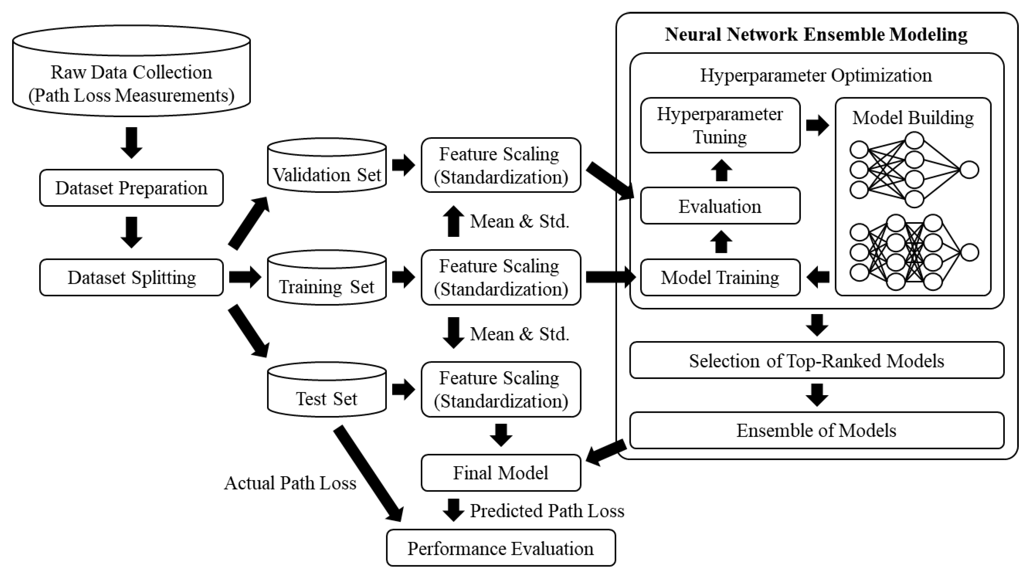
  • The entire process of predicting path loss using the proposed method is presented. The dataset splitting, feature scaling, and hyperparameter optimization processes have been detailed. Based on the results of the hyperparameter optimization process, the top-ranking ANNs can be determined. These results and the pseudocode for the proposed method can simplify re-implementation.
  • The proposed neural network ensemble model was quantitatively evaluated on a public dataset. Additionally, for benchmarking, nine ML-based path loss prediction methods were tested: SVM, k-NN, RF, decision tree, multiple linear regression, Least Absolute Shrinkage and Selection Operator (LASSO), ridge regression, Elastic Net, and ANNs.
The remainder of this paper is organized as follows. Section 2 reviews related studies, and Section 3 describes the proposed method for path loss prediction. Then, Section 4 details the experimental setup, including the evaluation metrics and implementation of the benchmark methods, and Section 5 presents and discusses the results. Finally, Section 6 provides the concluding remarks.

2. Related Work

2.1. Non-ANN-Based Path Loss Prediction

As previously mentioned, many different regression algorithms can predict path loss. Based on prior research, these algorithms can be classified into two groups: non-ANN-based and ANN-based. In a study on path loss prediction using non-ANN-based approach, a path loss equation consisting of several constants and simple functions was proposed [40]. Additionally, using a genetic algorithm, the authors identified constants and functions that fit the measurements well.
Instead of using a genetic algorithm, some researchers used an SVM for path loss prediction [41,42,43,44,45,46,47]. The authors of [41] proposed using an SVM with a radial basis function (RBF) kernel as a tool for predicting path loss. Generally, several types of kernels can be used in SVMs; the performance and effectiveness of the SVM depend on the kernel type. In [42], the authors compared the performances of three SVMs with different kernels: polynomial, Gaussian, and Laplacian. Their results revealed that SVM with a Laplacian kernel had outperformed the SVM with the other two kernels. Moreover, the authors compared the three SVMs with two empirical models (the Hata and Ericsson 9999 models); all three SVMs outperformed the empirical models. Motivated by the results of [41,42], the authors of [43,44,45,46,47] also used an SVM for path loss prediction.
The authors of [46,47,48] used k-NN, a well-known regression algorithm, for path loss prediction. In recent studies on non-ANN-based path loss prediction, ensemble methods that use multiple ML models to achieve better performances have garnered significant attention owing to their promising results. Based on empirical evidence, it is generally observed that ensemble methods achieve better performances when their constituent models are significantly diverse [49,50]. Consequently, several ensemble methods aim to enhance the diversity among their constituent models [51,52]. To this end, the authors of [53] proposed an ensemble method that averaged the results from five different regression algorithms: k-NN, SVM, RF, AdaBoost, and gradient boosting. Regarding RF, it is a widely used ensemble method that constructs numerous decision trees during the training phase. Additionally, during the testing phase, it derives the average prediction of individual trees as an output [54,55]. This method has been employed for path loss prediction [45,46,47,48].

2.2. ANN-Based Path Loss Prediction

Instead of using non-ANN-based approaches, several researchers have explored ANN-based methods for path loss prediction. In these approaches, hyperparameter tuning is crucial for ANNs because it directly affects their performance and generalization ability. Hyperparameters are configuration settings that are external to a model and cannot be learned from data. Unlike the weights and biases of an ANN, which are learned during the training phase, hyperparameters should be set prior to training. The hyperparameters of an ANN include the learning rate, batch size, number of hidden layers, the number of neurons in each layer, activation functions, dropout rates, and regularization strength.
To determine the optimal configuration that maximizes ANN performance, many researchers have conducted hyperparameter tuning in their studies. For example, the authors of [38,56,57] explored the relationship between ANN performance and the number of layers. Their results revealed that adding depth to an ANN by increasing the number of layers would enable accurate path loss prediction. The authors of [58] experimented with the performance of an ANN by varying the number of neurons in a hidden layer while keeping the number of hidden layers constant at one. According to their results, increasing the number of neurons improved the path loss prediction performance of the ANN. In [59], the authors proposed a differential evolution algorithm to determine the optimal number of neurons in each layer of an ANN that would achieve the best performance in path loss prediction.
Generally, activation functions are used to introduce nonlinearity into ANNs. The choice of an activation function significantly impacts the performance and generalization ability of an ANN. Several types of activation functions have been developed and used in ANNs. The RBF is a widely used activation function in path loss prediction. For example, the authors of [58,60,61] proposed an RBF neural network (RBF-NN), where the RBF was used as an activation function. In [62], the authors proposed a wavelet neural network for field-strength prediction using a wavelet function as an activation function. According to their results, the prediction performance of the wavelet neural network exceeded that of the RBF-NN. Other types of activation functions such as the hyperbolic tangent (tanh) [63,64,65,66,67,68,69,70] and sigmoid functions [71,72,73,74,75] have also been used in ANNs for path loss prediction.
Recently, several ANN variations, including the convolutional neural network (CNN), have been widely used for path loss prediction. A CNN typically consists of input, hidden, and output layers, with the hidden layers comprising one or more convolutional layers. In a convolutional layer, several convolution kernels (filters) can be used, and the dot product of each convolution kernel with the input matrix of the layer is obtained to generate feature maps. A rectified linear unit (ReLU) is commonly used as an activation function in convolutional layers; the activation maps for the feature maps are obtained by applying the ReLU, and these activation maps become the inputs to the next layer. Generally, the convolutional layer is followed by a pooling layer, and the pooling layer reduces the dimensions of data by combining the outputs of neuron clusters at one layer into a single neuron in the next layer. Through convolutional and pooling layers, CNNs can detect and extract meaningful features from images. Consequently, CNNs are commonly used to solve computer vision tasks, such as image classification and image recognition.
Owing to promising results from using CNNs in computer vision tasks, CNN-based methods have emerged in studies on path loss prediction. For example, the authors of [56] proposed a CNN-based method to predict the path loss exponent from a 3-D building map; two 2-D images obtained from a 3-D building map were utilized. One image was created by mapping the height of each building to an integer value within the range of 0–255, and the other was generated by mapping the difference between the height of the transmitter from sea level and the height of the ground from sea level to an integer value within the range of 0 to 255. The two images were stacked in the form of a 3-D tensor, which was used as the input for the CNN. The CNN was trained using synthetic data generated using a ray-tracing tool to predict the path loss exponent.
Recently, some popular CNN architectures proposed for computer vision tasks have been applied to path loss prediction. For example, the authors of [76] utilized AlexNet, which was proposed in [77], as the base model for path loss prediction. The model input consisted of a 3-D tensor constructed by stacking three 2-D matrices. These matrices contained information about the height of structures and buildings, the distance from the transmitter, and the distance from the receiver. Another study by the same authors employed AlexNet as the base model [78]. In this study, the 3-D tensor was augmented with a 2-D matrix containing information about the angle formed by the line between the transmitter and receiver. The Visual Geometry Group neural network (VGGNet) [79] is another well-known CNN architecture. It can be categorized into several architectures according to the number of convolutional layers. Among them, the VGG-16 and VGG-19 architectures are typically used because their performance is better than that of other VGGNet architectures. In [80], the authors utilized the VGG-16 architecture to predict the path loss distribution from 2-D satellite images. Motivated by the idea presented in [80], the authors of [81] employed the VGG-16 architecture as the backbone to predict the path loss exponent and shadowing factor from 2-D satellite images. The residual neural network (ResNet) [82] is also a widely used CNN architecture. The ResNet architecture was used in a similar study to predict the path loss exponent and shadowing factor from 2-D satellite images [83] and in another study [84] to predict the path loss from 2-D satellite images.

3. Proposed Method

3.1. Overall Process

This section details the working of the proposed path loss prediction method; Figure 1 shows a schematic overview of its process, which is divided into three phases: (1) dataset splitting and feature scaling, (2) model building and hyperparameter optimization, and (3) applying the ensemble model and performing path loss prediction. In the first phase, dataset splitting is conducted on the prepared dataset, producing training, validation, and test sets. Subsequently, feature scaling is applied to enhance the performance of the ANNs. In the second phase, the ANNs are built with different hyperparameter configurations; the hyperparameters include the number of hidden layers, number of neurons in each hidden layer, and type of activation function. During the hyperparameter optimization process, each ANN is trained and evaluated, and the results are recorded. In the final phase, the top-ranked ANNs are selected based on the evaluation results, and the final model is constructed using an ensemble of the selected ANNs. A path loss prediction is conducted on the test set using the final model.

3.2. Dataset Preparation

The dataset proposed by the authors in [85] was used in this study. To collect path loss data, these authors conducted a drive test measurement campaign at Covenant University, Ota, Ogun State, Nigeria. During the drive tests, measurements were performed along three different routes. During each measurement, the mobile station was moved away from each of the three base stations. These authors recorded terrain profile information, including longitude ( f 1 ), latitude ( f 2 ), elevation ( f 3 ), altitude ( f 4 ), clutter height ( f 5 ), and distance between the transmitter and receiver ( f 6 ), along with path loss data. Across the three routes, 937, 1229, and 1450 samples were collected; the dataset contained 3616 samples, comprising six features and path loss values as labels. In this study, we aimed to obtain a generalized neural network ensemble model rather than a site-specific model. To reach this goal, all 3616 samples were used without further divisions.

3.3. Dataset Splitting and Feature Scaling

In this study, the dataset was randomly shuffled and then split into training, validation, and testing sets. A training set was used to train the model. If the model was evaluated on the same data on which it had been trained, it might have performed well on that specific dataset but would have failed to generalize to new data (overfitting); the validation set helped detect and prevent this issue. Moreover, the validation set allowed the tuning of the hyperparameters without introducing bias from the test set. The test set provided an unbiased evaluation of the final performance of the model, indicating how well it would perform on new real-world data. Generally, separating data into training, validation, and test sets can ensure that ML models are robust, generalize well to new data, and perform reliably in real-world scenarios. More specifically, in our study, 60% of the 3616 samples were allocated to the training set, whereas 20% was assigned each to the validation and test sets.
Table 1 presents the descriptive statistics of the training dataset. As indicated in the table, the scales of the six features differed. Generally, if the features are on different scales, ML algorithms may assign greater importance to features with larger magnitudes. Additionally, these algorithms can be sensitive to the scale of the input features, thereby affecting their performance. To mitigate these issues, the features were standardized by removing the mean and scaling to the unit variance. Let x j = [ f 1 , j , f 2 , j , f 3 , j , f 4 , j , f 5 , j , f 6 , j ] be the jth sample in the dataset, where f 1 , j , f 2 , j , f 3 , j , f 4 , j , f 5 , j , and f 6 , j are the corresponding feature values of the jth sample. Then, the standard score of each feature value in x j is calculated as:
f ˜ i , j = ( f i , j f ¯ i ) σ i , i { 1 , 2 , 3 , 4 , 5 , 6 } ,
where f ¯ i is the mean of f i for the training samples, and σ i is the standard deviation of f i for the training samples.

3.4. Hyperparameter Optimization

Our proposed model consists of multiple ANNs, each of which can have multiple fully connected layers as hidden layers; every input neuron is connected to every output neuron, which is a configuration commonly used in ANNs. To construct the optimal ensemble structure, hyperparameter optimization processes were executed. The considered hyperparameters included the number of hidden layers, number of neurons in each hidden layer, and type of activation function. Throughout these processes, a training dataset was used to train each ANN. Early stopping was applied to prevent the training of the ANN for an excessive number of epochs, which could lead to overfitting; a validation dataset was used to detect and prevent overfitting. For each hyperparameter configuration, the mean squared error (MSE) of the ANN was computed for the validation dataset.
For clarity, let M be the number of hidden layers in the ANN and N be the number of neurons in each hidden layer. Figure 2 shows a heat map of the MSE values based on M and N. In the experiments shown in Figure 2a, the ReLU was used as the activation function in each hidden layer, and the ANN with M = 8 and N = 10 achieved the minimum MSE; in those shown in Figure 2b, a sigmoid function was used as the activation function and an ANN with M = 3 and N = 12 achieved the minimum MSE; and in those shown in Figure 2c, a hyperbolic tangent function was used, and the ANN with M = 1 and N = 22 achieved the optimal MSE. The results presented in Figure 2b,c showed that the MSE of the ANNs had never decreased below 79 for M values 4 .

3.5. Ensemble of Artificial Neural Networks

As illustrated in Figure 1, the proposed method involves a neural network ensemble model composed of multiple ANNs. To enhance the diversity among the integrated ANNs, the top T ANNs were selected based on the results of the hyperparameter optimization. For simplicity, hereafter, the selected top T ANNs shall be referred to as A N N 1 , A N N 2 , A N N 3 , ⋯, A N N T 1 , and A N N T . Table 2 lists the hyperparameter configurations and MSE of the 20 highest-ranking ANNs.
The pseudocode for the proposed neural network ensemble method is presented in Algorithm 1. As shown in the pseudocode, the given dataset was split into training, validation, and test sets. Feature scaling was applied to each set using Equation (1). Subsequently, various ANNs were constructed with different hyperparameter configurations. Each ANN was trained using a training dataset and evaluated on the validation dataset, and the MSE results were recorded. The top-ranked ANNs were selected based on their MSE results, and the final model was constructed using an ensemble of the selected ANNs.
Algorithm 1 Pseudocode for the proposed neural network ensemble method
Input:  Dataset D
Output:  Final ensemble model E
1:
Split D into training, validation, and test sets ( D t r a i n i n g , D v a l i d a t i o n , and D t e s t , respectively)
2:
Determine f ¯ i and σ i
3:
Apply feature scaling to D t r a i n i n g , D v a l i d a t i o n , and D t e s t using Equation (1)
4:
Set T, M, and N
5:
Set the maximum epochs ( m a x _ e p o c h s )
6:
Set the number of training samples in the batch ( b a t c h _ s i z e )
7:
Create an early stopping callback ( e s _ c b )
8:
Create an empty list H
9:
for  m = 0 to M do
10:
   for  n = 1 to N do
11:
       for  a c t i v a t i o n in {“ReLU”, “sigmoid”, “tanh”} do
12:
           m o d e l = Build_Neural_Network(m, n, a c t i v a t i o n )
13:
           m o d e l = Training( m o d e l , D t r a i n i n g , D v a l i d a t i o n , m a x _ e p o c h s , b a t c h _ s i z e , e s _ c b )
14:
           v a l _ l o s s = Evaluation( m o d e l , D v a l i d a t i o n )
15:
          Append [ v a l _ l o s s , m o d e l ] to H
16:
       end for
17:
   end for
18:
end for
19:
Sort each m o d e l in ascending order based on the v a l _ l o s s recorded on H
20:
Select the top-ranked T models
21:
E = Build_Ensemble(selected T models)
22:
return E
The key concept behind the proposed neural network ensemble model was training multiple ANNs with different subsets of hyperparameters and aggregating their predictions. Through this process, the proposed model became more robust and less prone to overfitting. The ensemble nature of the model helped improve the generalization and predictive performance. During the prediction phase, each ANN in the ensemble independently predicted input data. The predictions from all ANNs were then aggregated to produce the final prediction. In this study, the final output of the neural network ensemble model was the average of the predictions made by each ANN. For clarity, let y ^ r be the path loss value predicted by A N N r . Then, the predicted path loss values from T ANNs can be represented as vector Y ^ as follows:
Y ^ = [ y ^ 1 , y ^ 2 , , y ^ T 1 , y ^ T ] .
To derive the final prediction result from Y ^ in Equation (2), the predictions of T ANNs were averaged.

4. Experimental Setup

4.1. Evaluation Metrics

Generally, using multiple metrics in the performance evaluation of algorithms provides a more comprehensive and nuanced understanding of their performance; relying on a single metric may result in an incomplete or biased assessment. Therefore, for our performance evaluation, we utilized various metrics, including the MSE, root mean square error (RMSE), mean absolute error (MAE), mean absolute percentage error (MAPE), mean squared logarithmic error (MSLE), root mean squared logarithmic error (RMSLE), and coefficient of determination. For clarity, let y j be the actual path loss value for the jth sample x j in the dataset, y ¯ j be the predicted path loss value for x j , and S be the total number of y ¯ j generated from S samples in the dataset. Subsequently, the MSE, which measures the average of the squares of the errors, can be computed using the following formula:
M S E = 1 S j = 1 S ( y j y ¯ j ) 2 .
Although the RMSE and MSE are similar in terms of model scoring, they are not always immediately interchangeable, with MSE tending to be more sensitive to outliers, treating all errors equally regardless of their magnitude. If outliers are present in the dataset, MSE may be influenced more by these extreme values. In contrast, the RMSE tends to be less sensitive to outliers because it involves the square root of the squared errors; the RMSE is defined as the square root of the MSE, as follows:
R M S E = M S E = 1 S j = 1 S ( y j y ¯ j ) 2 .
Compared with the MSE, the MAE is less sensitive to outliers because each error term contributes equally to the overall error because it is based on absolute differences; the MAE is defined as the average of the absolute errors:
M A E = 1 S j = 1 S | y j y ¯ j | .
Regarding the MAPE, it is defined as follows:
M A P E = 1 S j = 1 S | y j y ¯ j y j | .
Then, the MSLE, which measures the mean of the squared logarithmic differences between y j and y ¯ j , can be computed as follows:
M S L E = 1 S j = 1 S { log ( y j + 1 ) log ( y ¯ j + 1 ) } 2 .
Concerning the RMSLE, it is defined as the square root of the MSLE, as follows:
R M S L E = M S L E = 1 S j = 1 S { log ( y j + 1 ) log ( y ¯ j + 1 ) } 2 .
The coefficient of determination, which is denoted by R 2 , is defined as follows:
R 2 = 1 j = 1 S ( y j y ¯ j ) 2 j = 1 S ( y j y ¯ ) 2 ,
where y ¯ is the mean of the actual path loss values in the dataset (i.e., y ¯ = 1 / S × j = 1 S y j ), and R 2 is typically used as a measure of the goodness-of-fit of a model, with an R 2 value of 1 indicating that the predictions of the model fit the actual data perfectly.

4.2. Implementation of Benchmark Methods

In our experiments, to compare the performance of the proposed method, we implemented nine path loss prediction methods: (1) SVM-based, (2) k-NN-based, (3) RF-based, (4) decision tree (DT)-based, (5) multiple linear regression (MLR)-based, (6) LASSO-based, (7) ridge regression-based, (8) Elastic Net-based, and (9) ANN-based methods. To achieve this, the scikit-learn ML library for Python was utilized. The optimal hyperparameter configuration for each model was determined using the HalvingGridSearchCV class. The nine methods are detailed below.

4.2.1. SVM-Based Path Loss Prediction Method

An SVM was employed for path loss prediction in [41,42,43,44,45,46,47]. In our study, an SVM was implemented using an SVR class in the scikit-learn library. The SVR class is an implementation of epsilon-support vector regression and includes various hyperparameters, such as the kernel type, kernel coefficient, and regularization parameter. Table 3 presents the optimal hyperparameter combinations for SVM, as determined through the hyperparameter optimization process.

4.2.2. k-NN-Based Path Loss Prediction Method

The k-NN was employed for path loss prediction in [46,47,48]. It was implemented using the KNeighborsRegressor class in the scikit-learn library. This class includes various hyperparameters such as the number of neighbors, type of weight function used in the prediction, and type of metric used for distance computation. Table 4 presents the optimal hyperparameter combination for k-NN, as determined using the hyperparameter optimization process.

4.2.3. RF-Based Path Loss Prediction Method

The RF technique was employed for path loss prediction in [45,46,47,48]. In our study, it was implemented using the RandomForestRegressor class in the scikit-learn library. This class includes various hyperparameters, such as the number of decision trees in the model, the type of function used to measure the quality of a split, and the maximum depth of the tree. Table 5 presents the optimal hyperparameter combination for RF, as determined through the hyperparameter optimization process.

4.2.4. DT-Based Path Loss Prediction Method

A DT predicts a continuous value by recursively partitioning the data based on the input features and creating a tree structure in which each leaf node contains the predicted value for instances that follow the path to that leaf. It can also be employed for path loss prediction. In our study, DT was implemented using the DecisionTreeRegressor class in the scikit-learn library. This class includes various hyperparameters, such as the type of function used to measure the quality of a split, the strategy used to choose the split at each node, and the maximum depth of the tree. Table 6 presents the optimal hyperparameter combination for DT, as determined through the hyperparameter optimization process.

4.2.5. MLR-Based Path Loss Prediction Method

Multiple Linear Regression (MLR) is an extension of simple linear regression, which models the relationship between a dependent variable and multiple independent variables. In a simple linear regression, there is only one independent variable, whereas in multiple linear regression, there are two or more independent variables. The coefficients of the independent variables and the y-intercept are estimated from the training samples using methods such as the least-squares method, which minimizes the MSE. Regarding MLR, it is widely used in various fields to predict outcomes, understand the relationships between variables, and determine the strength and significance of these relationships. In our study, MLR was implemented using the LinearRegression class in the scikit-learn library and employed as a benchmark method. Table 7 presents the optimal hyperparameter combination for MLR, as determined by the hyperparameter optimization process.

4.2.6. LASSO-Based Path Loss Prediction Method

The LASSO regularization technique is used in linear regression to prevent overfitting and encourage simpler models. Linear regression is performed to determine the coefficients of the independent variables that best fit the observed data. Regarding LASSO, it introduces a penalty term for the traditional linear regression objective function. The penalty term, denoted by L1, is proportional to the absolute values of the coefficients. For brevity, the linear regression model trained with L1 was named LASSO. LASSO was implemented using the LASSO class in the scikit-learn library and employed as a benchmark method. Table 8 presents the optimal hyperparameter combination for LASSO, as determined through the hyperparameter optimization process.

4.2.7. Ridge-Based Path Loss Prediction Method

Ridge regression, also known as Tikhonov regularization, is a technique used in linear regression to address multicollinearity and prevent overfitting. Like LASSO, ridge regression introduces a penalty term to the traditional linear regression objective function. The penalty term, denoted by L2, is proportional to the square of the coefficient. Unlike LASSO, ridge regression does not force the coefficients to be zero. Instead, it reduces the coefficients toward zero, thereby reducing their magnitudes. Advantageously, ridge regression can handle multicollinearity, which occurs when the independent variables in a regression model are highly correlated. Multicollinearity can also lead to unstable and unreliable coefficient estimates. The ridge regression adds a penalty term to the objective function, which mitigates the impact of multicollinearity by discouraging overly large coefficients. For brevity, the linear regression model trained with L2 was named Ridge. It was implemented using the Ridge class in the scikit-learn library and employed as a benchmark method. Table 9 presents the optimal hyperparameter combination for MLR, as determined through the hyperparameter optimization process.

4.2.8. Elastic Net-Based Path Loss Prediction Method

Elastic Net is a regularization technique used in linear regression that combines both the L1 (LASSO) and L2 (Ridge) regularization penalties. It is designed to find a balance between LASSO and Ridge regression and thereby overcome some of their limitations. Elastic Net introduces a new hyperparameter that controls the combination of L1 and L2 penalties. The regularization term in the Elastic Net is a linear combination of both penalties. In this study, an Elastic Net was implemented using the ElasticNet class in the scikit-learn library and used as the benchmark method. Table 10 presents the optimal hyperparameter combinations for the Elastic Net determined through the hyperparameter optimization process.

4.2.9. ANN-Based Path Loss Prediction Method

As previously noted, ANNs have been employed for path loss prediction [38,56,57,58,59,60,61,62,63,64,65,66,67,68,69,70,71,72,73,74,75]. Based on the details of hyperparameter configurations for ANNs in existing research, ANNs were implemented in our study using the TensorFlow library and employed as benchmarks. Table 11 lists the hyperparameter combinations for the ANNs.

5. Results and Discussion

Table 12 lists the performance metrics for the ensemble models with different numbers of ANNs; it shows that the best performance of the proposed ensemble model was when T = 20 . Therefore, in this study, the optimal value of T was set as 20. In other words, the proposed ensemble model consisted of 20 A N N r models ( r { 1 , 2 , , 19 , 20 } ). Clearly, the performance of the ensemble model increased as the number of ANNs increased. However, when the number of ANNs exceeded 20, the performance of the ensemble model did not improve further. Based on these results, an ensemble model consisting of 20 ANNs was selected as the final model.
Table 13 lists the MSE, RMSE, MAE, MAPE, MSLE, RMSLE, and R 2 of each path loss prediction method. Clearly, the proposed ensemble model performed the best across all evaluation metrics. This was because the ensemble model comprised the top-ranked ANNs selected based on the MSE results, thereby enhancing the diversity among the integrated ANNs and enabling the model to achieve a robust and accurate path loss prediction performance. Among the considered benchmark methods, the k-NN-based method achieved the best performance, whereas the ANN-based method with the hyperparameters described in [38] achieved the worst performance. The MAE of the proposed method was approximately 1.2753, whereas that of the k-NN-based method was 2.4983. The MAE of the proposed method was approximately 1.223 less than that of the k-NN-based method. The results in Table 13 revealed that the proposed method could predict path loss accurately.
Figure 3 shows the measured and predicted path loss for three survey routes. In the figure, the values of the measured path loss data were plotted against the corresponding distance. To achieve this, we sorted the data in the test set by the distance between the transmitter and receiver after splitting the test set according to the survey route. In all survey routes, the receiver encountered non-line-of-sight (NLoS) conditions, attributed to obstructions such as buildings and trees. From the figure, it is seen that the prediction performance of the proposed method aligns closely with the measured data. This result is consistent with the performance shown in Table 13.

6. Conclusions

In this study, we propose a novel ML-based method for path loss prediction. Our approach leveraged the power of neural network ensemble learning and provided a robust and accurate prediction model. By constructing an ensemble of neural networks and selecting the top-ranked networks based on a hyperparameter optimization process, the method achieved a state-of-the-art performance in path loss prediction, as evidenced by the results of rigorous validation on a publicly available dataset. Furthermore, we comprehensively compared its performance with that of various ML-based methods. The simulation results demonstrated the superior performance of the proposed method. Future research directions may explore fine tuning the model, considering additional parameters, and expanding the dataset to ensure the generalizability of the proposed method across diverse scenarios.

Author Contributions

Conceptualization, B.K. and H.S.; methodology, B.K.; software, B.K.; validation, B.K.; formal analysis, B.K.; investigation, B.K.; resources, B.K.; data curation, B.K.; writing—original draft preparation, B.K.; writing—review and editing, B.K.; visualization, B.K.; supervision, H.S.; project administration, H.S.; funding acquisition, H.S. All authors have read and agreed to the published version of the manuscript.

Funding

This research was supported by the National Research Foundation of Korea (NRF) grant funded by the Korea government (MSIT) (No.2021R1F1A1051075).

Institutional Review Board Statement

Not applicable.

Informed Consent Statement

Not applicable.

Conflicts of Interest

The authors declare no conflicts of interest.

References

  1. Son, H.; Lee, S. Bandwidth and region division for broadband multi-cell networks. IEEE Commun. Lett. 2006, 10, 360–362. [Google Scholar]
  2. Kwon, B.; Kim, S.; Lee, H.; Lee, S. A downlink power control algorithm for long-term energy efficiency of small cell network. Wirel. Netw. 2015, 21, 2223–2236. [Google Scholar] [CrossRef]
  3. Kwon, B.; Kim, S.; Jeon, D.; Lee, S. Iterative interference cancellation and channel estimation in evolved multimedia broadcast multicast system using filter-bank multicarrier-quadrature amplitude modulation. IEEE Trans. Broadcast. 2016, 62, 864–875. [Google Scholar] [CrossRef]
  4. Kwon, B.; Kim, S.; Lee, S. Scattered reference symbol-based channel estimation and equalization for FBMC-QAM systems. IEEE Trans. Commun. 2017, 65, 3522–3537. [Google Scholar] [CrossRef]
  5. Kwon, B.; Lee, S. Cross-antenna interference cancellation and channel estimation for MISO-FBMC/QAM-based eMBMS. Wirel. Netw. 2018, 24, 3281–3293. [Google Scholar] [CrossRef]
  6. Loh, W.R.; Lim, S.Y.; Rafie, I.F.M.; Ho, J.S.; Tze, K.S. Intelligent base station placement in urban areas with machine learning. IEEE Antennas Wirel. Propag. Lett. 2023, 22, 2220–2224. [Google Scholar] [CrossRef]
  7. Srinivasa, S.; Haenggi, M. Path loss exponent estimation in large wireless networks. In Proceedings of the IEEE Information Theory and Applications Workshop, La Jolla, CA, USA, 8–13 February 2009; pp. 124–129. [Google Scholar]
  8. Egli, J.J. Radio propagation above 40 MC over irregular terrain. Proc. IRE 1957, 45, 1383–1391. [Google Scholar] [CrossRef]
  9. Hata, M. Empirical formula for propagation loss in land mobile radio services. IEEE Trans. Veh. Technol. 1980, 29, 317–325. [Google Scholar] [CrossRef]
  10. Longley, A.G. Prediction of Tropospheric Radio Transmission Loss over Irregular Terrain: A Computer Method-1968; Institute for Telecommunication Sciences: Boulder, CO, USA, 1968; pp. 1–147. [Google Scholar]
  11. Okumura, Y. Field strength and its variability in VHF and UHF land-mobile radio service. Rev. Electr. Commun. Lab. 1968, 16, 825–873. [Google Scholar]
  12. 3GPP. Study on Channel Model for Frequencies from 0.5 to 100 GHz (Release 16) V16.1.0; Technical Report; Rep. TR 38.901; 3GPP: Sophia Antipolis, France, 2020. [Google Scholar]
  13. Zhu, Q.; Wang, C.X.; Hua, B.; Mao, K.; Jiang, S.; Yao, M. 3GPP TR 38.901 Channel Model. In The Wiley 5G Ref: The Essential 5G Reference Online; Wiley Press: Hoboken, NJ, USA, 2021; pp. 1–35. [Google Scholar]
  14. Riviello, D.G.; Di Stasio, F.; Tuninato, R. Performance analysis of multi-user MIMO schemes under realistic 3GPP 3-D channel model for 5G mmwave cellular networks. Electronics 2022, 11, 330. [Google Scholar] [CrossRef]
  15. Green, D.; Yun, Z.; Iskander, M.F. Path loss characteristics in urban environments using ray-tracing methods. IEEE Antennas Wirel. Propag. Lett. 2017, 16, 3063–3066. [Google Scholar] [CrossRef]
  16. Qian, J.; Wu, Y.; Saleem, A.; Zheng, G. Path loss model for 3.5 GHz and 5.6 GHz bands in cascaded tunnel environments. Sensors 2022, 22, 4524. [Google Scholar] [CrossRef] [PubMed]
  17. Timmins, I.J.; O’Young, S. Marine communications channel modeling using the finite-difference time domain method. IEEE Trans. Veh. Technol. 2008, 58, 2626–2637. [Google Scholar] [CrossRef]
  18. Kwon, B.; Kim, J.; Lee, K.; Lee, Y.K.; Park, S.; Lee, S. Implementation of a virtual training simulator based on 360° multi-view human action recognition. IEEE Access 2017, 5, 12496–12511. [Google Scholar] [CrossRef]
  19. Kwon, B.; Song, H.; Lee, S. Accurate blind Lempel-Ziv-77 parameter estimation via 1-D to 2-D data conversion over convolutional neural network. IEEE Access 2020, 8, 43965–43979. [Google Scholar] [CrossRef]
  20. Kwon, B.; Lee, S. Human skeleton data augmentation for person identification over deep neural network. Appl. Sci. 2020, 10, 4849. [Google Scholar] [CrossRef]
  21. Kwon, B.; Lee, S. Ensemble learning for skeleton-based body mass index classification. Appl. Sci. 2020, 10, 7812. [Google Scholar] [CrossRef]
  22. Kwon, B.; Lee, S. Joint swing energy for skeleton-based gender classification. IEEE Access 2021, 9, 28334–28348. [Google Scholar] [CrossRef]
  23. Kwon, B.; Huh, J.; Lee, K.; Lee, S. Optimal camera point selection toward the most preferable view of 3-d human pose. IEEE Trans. Syst. Man, Cybern. Syst. 2022, 52, 533–553. [Google Scholar] [CrossRef]
  24. Kwon, B.; Kim, T. Toward an online continual learning architecture for intrusion detection of video surveillance. IEEE Access 2022, 10, 89732–89744. [Google Scholar] [CrossRef]
  25. Cambria, E.; White, B. Jumping NLP curves: A review of natural language processing research. IEEE Comput. Intell. Mag. 2014, 9, 48–57. [Google Scholar] [CrossRef]
  26. Otter, D.W.; Medina, J.R.; Kalita, J.K. A survey of the usages of deep learning for natural language processing. IEEE Trans. Neural Netw. Learn. Syst. 2020, 32, 604–624. [Google Scholar] [CrossRef] [PubMed]
  27. Deng, J.; Ren, F. A survey of textual emotion recognition and its challenges. IEEE Trans. Affect. Comput. 2023, 14, 49–67. [Google Scholar] [CrossRef]
  28. Liu, Y.; Bi, S.; Shi, Z.; Hanzo, L. When machine learning meets big data: A wireless communication perspective. IEEE Veh. Technol. Mag. 2019, 15, 63–72. [Google Scholar] [CrossRef]
  29. Sun, Y.; Peng, M.; Zhou, Y.; Huang, Y.; Mao, S. Application of machine learning in wireless networks: Key techniques and open issues. IEEE Commun. Surv. Tutorials 2019, 21, 3072–3108. [Google Scholar] [CrossRef]
  30. Yang, H.; Xie, X.; Kadoch, M. Machine learning techniques and a case study for intelligent wireless networks. IEEE Netw. 2020, 34, 208–215. [Google Scholar] [CrossRef]
  31. Zhu, G.; Liu, D.; Du, Y.; You, C.; Zhang, J.; Huang, K. Toward an intelligent edge: Wireless communication meets machine learning. IEEE Commun. Mag. 2020, 58, 19–25. [Google Scholar] [CrossRef]
  32. Hu, S.; Chen, X.; Ni, W.; Hossain, E.; Wang, X. Distributed machine learning for wireless communication networks: Techniques, architectures, and applications. IEEE Commun. Surv. Tutorials 2021, 23, 1458–1493. [Google Scholar] [CrossRef]
  33. Li, J.; Zhang, X. Deep reinforcement learning-based joint scheduling of eMBB and URLLC in 5G networks. IEEE Wirel. Commun. Lett. 2020, 9, 1543–1546. [Google Scholar] [CrossRef]
  34. Xu, Y.; Xu, W.; Wang, Z.; Lin, J.; Cui, S. Load balancing for ultradense networks: A deep reinforcement learning-based approach. IEEE Internet Things J. 2019, 6, 9399–9412. [Google Scholar] [CrossRef]
  35. Spantideas, S.T.; Giannopoulos, A.E.; Kapsalis, N.C.; Kalafatelis, A.; Capsalis, C.N.; Trakadas, P. Joint energy-efficient and throughput-sufficient transmissions in 5G cells with deep Q-learning. In Proceedings of the IEEE International Mediterranean Conference on Communications and Networking (MeditCom), Athens, Greece, 7–10 September 2021; pp. 265–270. [Google Scholar]
  36. Kaloxylos, A.; Gavras, A.; Camps, D.; Ghoraishi, M.; Hrasnica, H. AI and ML–Enablers for beyond 5G Networks. 5G PPP Technol. Board 2021, 1, 1–145. [Google Scholar]
  37. Li, X.; Fang, J.; Cheng, W.; Duan, H.; Chen, Z.; Li, H. Intelligent power control for spectrum sharing in cognitive radios: A deep reinforcement learning approach. IEEE Access 2018, 6, 25463–25473. [Google Scholar] [CrossRef]
  38. Ostlin, E.; Zepernick, H.J.; Suzuki, H. Macrocell path-loss prediction using artificial neural networks. IEEE Trans. Veh. Technol. 2010, 59, 2735–2747. [Google Scholar] [CrossRef]
  39. Isabona, J.; Srivastava, V.M. Hybrid neural network approach for predicting signal propagation loss in urban microcells. In Proceedings of the IEEE Region 10 Humanitarian Technology Conference (R10-HTC), Agra, India, 21–23 December 2016; pp. 1–5. [Google Scholar]
  40. Fernandes, L.C.; Soares, A.J.M. A hybrid model for path loss calculation in urban environment. In Proceedings of the 17th International Conference on the Computation of Electromagnetic Fields (COMPUMAG), Florianópolis, Brazil, 22–26 November 2009; pp. 460–461. [Google Scholar]
  41. Piacentini, M.; Rinaldi, F. Path loss prediction in urban environment using learning machines and dimensionality reduction techniques. Comput. Manag. Sci. 2011, 8, 371–385. [Google Scholar] [CrossRef]
  42. Timoteo, R.D.; Cunha, D.C.; Cavalcanti, G.D. A proposal for path loss prediction in urban environments using support vector regression. In Proceedings of the 10th Advanced International Conference on Telecommunications (AICT), Paris, France, 20–24 July 2014; pp. 1–5. [Google Scholar]
  43. Gideon, K.; Nyirenda, C.; Temaneh-Nyah, C. Echo state network-based radio signal strength prediction for wireless communication in northern Namibia. IET Commun. 2017, 11, 1920–1926. [Google Scholar] [CrossRef]
  44. Famoriji, O.J.; Shongwe, T. Path Loss Prediction in Tropical Regions using Machine Learning Techniques: A Case Study. Electronics 2022, 11, 2711. [Google Scholar] [CrossRef]
  45. Wen, J.; Zhang, Y.; Yang, G.; He, Z.; Zhang, W. Path loss prediction based on machine learning methods for aircraft cabin environments. IEEE Access 2019, 7, 159251–159261. [Google Scholar] [CrossRef]
  46. Moreta, C.E.G.; Acosta, M.R.C.; Koo, I. Prediction of digital terrestrial television coverage using machine learning regression. IEEE Trans. Broadcast. 2019, 65, 702–712. [Google Scholar] [CrossRef]
  47. Elmezughi, M.K.; Salih, O.; Afullo, T.J.; Duffy, K.J. Comparative analysis of major machine-learning-based path loss models for enclosed indoor channels. Sensors 2022, 22, 4967. [Google Scholar] [CrossRef]
  48. Oroza, C.A.; Zhang, Z.; Watteyne, T.; Glaser, S.D. A machine-learning-based connectivity model for complex terrain large-scale low-power wireless deployments. IEEE Trans. Cogn. Commun. Netw. 2017, 3, 576–584. [Google Scholar] [CrossRef]
  49. Sollich, P.; Krogh, A. Learning with ensembles: How overfitting can be useful. In Proceedings of the Advances in Neural Information Processing Systems (NIPS), Denver, CO, USA, 27–30 November 1995; pp. 190–196. [Google Scholar]
  50. Kuncheva, L.I.; Whitaker, C.J. Measures of diversity in classifier ensembles and their relationship with the ensemble accuracy. Mach. Learn. 2003, 51, 181–207. [Google Scholar] [CrossRef]
  51. Brown, G.; Wyatt, J.; Harris, R.; Yao, X. Diversity creation methods: A survey and categorisation. Inf. Fusion 2005, 6, 5–20. [Google Scholar] [CrossRef]
  52. Adeva, J.J.G.; Beresi, U.C.; Calvo, R.A. Accuracy and diversity in ensembles of text categorisers. CLEI Electron. J. 2005, 8, 1–12. [Google Scholar]
  53. Karra, D.; Goudos, S.K.; Tsoulos, G.V.; Athanasiadou, G. Prediction of received signal power in mobile communications using different machine learning algorithms: A comparative study. In Proceedings of the IEEE Panhellenic Conference on Electronics & Telecommunications (PACET), Volos, Greece, 8–9 November 2019; pp. 1–4. [Google Scholar]
  54. Ho, T.K. Random decision forests. In Proceedings of the IEEE International Conference on Document Analysis and Recognition, Montreal, QC, Canada, 14–16 August 1995; pp. 278–282. [Google Scholar]
  55. Ho, T.K. The random subspace method for constructing decision forests. IEEE Trans. Pattern Anal. Mach. Intell. 1998, 20, 832–844. [Google Scholar]
  56. Lee, J.Y.; Kang, M.Y.; Kim, S.C. Path loss exponent prediction for outdoor millimeter wave channels through deep learning. In Proceedings of the IEEE Wireless Communications and Networking Conference (WCNC), Marrakesh, Morocco, 15–18 April 2019; pp. 1–5. [Google Scholar]
  57. Wu, L.; He, D.; Guan, K.; Ai, B.; Briso-Rodríguez, C.; Shui, T.; Liu, C.; Zhu, L.; Shen, X. Received power prediction for suburban environment based on neural network. In Proceedings of the IEEE International Conference on Information Networking (ICOIN), Barcelona, Spain, 7–10 January 2020; pp. 35–39. [Google Scholar]
  58. Chang, P.R.; Yang, W.H. Environment-adaptation mobile radio propagation prediction using radial basis function neural networks. IEEE Trans. Veh. Technol. 1997, 46, 155–160. [Google Scholar] [CrossRef]
  59. Sotiroudis, S.P.; Goudos, S.K.; Gotsis, K.A.; Siakavara, K.; Sahalos, J.N. Application of a composite differential evolution algorithm in optimal neural network design for propagation path-loss prediction in mobile communication systems. IEEE Antennas Wirel. Propag. Lett. 2013, 12, 364–367. [Google Scholar] [CrossRef]
  60. Popescu, I.; Kanstas, A.; Angelou, E.; Nafornita, L.; Constantinou, P. Applications of generalized RBF-NN for path loss prediction. In Proceedings of the 13th IEEE International Symposium on Personal, Indoor and Mobile Radio Communications, Lisbon, Portugal, 18 September 2002; pp. 484–488. [Google Scholar]
  61. Zaarour, N.; Kandil, N.; Hakem, N.; Despins, C. Comparative experimental study on modeling the path loss of an UWB channel in a mine environment using MLP and RBF neural networks. In Proceedings of the IEEE International Conference on Wireless Communications in Underground and Confined Areas, Clermont-Ferrand, France, 28–30 August 2012; pp. 1–6. [Google Scholar]
  62. Cheng, F.; Shen, H. Field strength prediction based on wavelet neural network. In Proceedings of the 2nd IEEE International Conference on Education Technology and Computer, Shanghai, China, 22–24 June 2010; pp. 255–258. [Google Scholar]
  63. Balandier, T.; Caminada, A.; Lemoine, V.; Alexandre, F. 170 MHz field strength prediction in urban environment using neural nets. In Proceedings of the 6th IEEE International Symposium on Personal, Indoor and Mobile Radio Communications, Toronto, ON, Canada, 27–29 September 1995; pp. 120–124. [Google Scholar]
  64. Panda, G.; Mishra, R.K.; Palai, S.S. A novel site adaptive propagation model. IEEE Antennas Wirel. Propag. Lett. 2005, 4, 447–448. [Google Scholar] [CrossRef]
  65. Kalakh, M.; Kandil, N.; Hakem, N. Neural networks model of an UWB channel path loss in a mine environment. In Proceedings of the 75th IEEE Vehicular Technology Conference (VTC Spring), Yokohama, Japan, 6–9 May 2012; pp. 1–5. [Google Scholar]
  66. Azpilicueta, L.; Rawat, M.; Rawat, K.; Ghannouchi, F.M.; Falcone, F. A ray launching-neural network approach for radio wave propagation analysis in complex indoor environments. IEEE Trans. Antennas Propag. 2014, 62, 2777–2786. [Google Scholar] [CrossRef]
  67. Ayadi, M.; Zineb, A.B.; Tabbane, S. A UHF path loss model using learning machine for heterogeneous networks. IEEE Trans. Antennas Propag. 2017, 65, 3675–3683. [Google Scholar] [CrossRef]
  68. Popoola, S.I.; Jefia, A.; Atayero, A.A.; Kingsley, O.; Faruk, N.; Oseni, O.F.; Abolade, R.O. Determination of neural network parameters for path loss prediction in very high frequency wireless channel. IEEE Access 2019, 7, 150462–150483. [Google Scholar] [CrossRef]
  69. Ebhota, V.C.; Isabona, J.; Srivastava, V.M. Environment-adaptation based hybrid neural network predictor for signal propagation loss prediction in cluttered and open urban microcells. Wirel. Pers. Commun. 2019, 104, 935–948. [Google Scholar] [CrossRef]
  70. Zhang, Y.; Wen, J.; Yang, G.; He, Z.; Wang, J. Path loss prediction based on machine learning: Principle, method, and data expansion. Appl. Sci. 2019, 9, 1908. [Google Scholar] [CrossRef]
  71. Wu, D.; Zhu, G.; Ai, B. Application of artificial neural networks for path loss prediction in railway environments. In Proceedings of the 5th IEEE International ICST Conference on Communications and Networking in China, Beijing, China, 25–27 August 2010; pp. 1–5. [Google Scholar]
  72. Zineb, A.B.; Ayadi, M. A multi-wall and multi-frequency indoor path loss prediction model using artificial neural networks. Arab. J. Sci. Eng. 2016, 41, 987–996. [Google Scholar] [CrossRef]
  73. Liu, J.; Jin, X.; Dong, F.; He, L.; Liu, H. Fading channel modelling using single-hidden layer feedforward neural networks. Multidimens. Syst. Signal Process. 2017, 28, 885–903. [Google Scholar] [CrossRef]
  74. Gómez-Pérez, P.; Crego-García, M.; Cuiñas, I.; Caldeirinha, R.F. Modeling and inferring the attenuation induced by vegetation barriers at 2G/3G/4G cellular bands using artificial neural networks. Measurement 2017, 98, 262–275. [Google Scholar] [CrossRef]
  75. Adeogun, R. Calibration of stochastic radio propagation models using machine learning. IEEE Antennas Wirel. Propag. Lett. 2019, 18, 2538–2542. [Google Scholar] [CrossRef]
  76. Kuno, N.; Takatori, Y. Prediction method by deep-learning for path loss characteristics in an open-square environment. In Proceedings of the IEEE International Symposium on Antennas and Propagation (ISAP), Busan, Republic of Korea, 23–26 October 2018; pp. 1–2. [Google Scholar]
  77. Krizhevsky, A.; Sutskever, I.; Hinton, G.E. ImageNet classification with deep convolutional neural networks. Commun. ACM 2017, 60, 84–90. [Google Scholar] [CrossRef]
  78. Kuno, N.; Yamada, W.; Sasaki, M.; Takatori, Y. Convolutional neural network for prediction method of path loss characteristics considering diffraction and reflection in an open-square environment. In Proceedings of the IEEE URSI Asia-Pacific Radio Science Conference (AP-RASC), New Delhi, India, 9–15 March 2019; pp. 1–3. [Google Scholar]
  79. Simonyan, K.; Zisserman, A. Very deep convolutional networks for large-scale image recognition. In Proceedings of the 3rd International Conference on Learning Representations (ICLR), San Diego, CA, USA, 7–9 May 2015; pp. 1–14. [Google Scholar]
  80. Ahmadien, O.; Ates, H.F.; Baykas, T.; Gunturk, B.K. Predicting path loss distribution of an area from satellite images using deep learning. IEEE Access 2020, 8, 64982–64991. [Google Scholar] [CrossRef]
  81. Bal, M.; Marey, A.; Ates, H.F.; Baykas, T.; Gunturk, B.K. Regression of large-scale path loss parameters using deep neural networks. IEEE Antennas Wirel. Propag. Lett. 2022, 21, 1562–1566. [Google Scholar] [CrossRef]
  82. He, K.; Zhang, X.; Ren, S.; Sun, J. Deep residual learning for image recognition. In Proceedings of the IEEE Conference on Computer Vision and Pattern Recognition (CVPR), Las Vegas, NV, USA, 27–30 June 2016; pp. 770–778. [Google Scholar]
  83. Ates, H.F.; Hashir, S.M.; Baykas, T.; Gunturk, B.K. Path loss exponent and shadowing factor prediction from satellite images using deep learning. IEEE Access 2019, 7, 101366–101375. [Google Scholar] [CrossRef]
  84. Sani, U.S.; Malik, O.A.; Lai, D.T.C. Improving path loss prediction using environmental feature extraction from satellite images: Hand-crafted vs. convolutional neural network. Appl. Sci. 2022, 12, 7685. [Google Scholar] [CrossRef]
  85. Popoola, S.I.; Atayero, A.A.; Arausi, O.D.; Matthews, V.O. Path loss dataset for modeling radio wave propagation in smart campus environment. Data Brief 2018, 17, 1062–1073. [Google Scholar] [CrossRef] [PubMed]
Figure 1. Overall working of the proposed method for path loss prediction.
Sensors 24 00304 g001
Figure 2. Heat map of MSE values based on M and N: (a) ReLU, (b) sigmoid, and (c) tanh.
Sensors 24 00304 g002aSensors 24 00304 g002b
Figure 3. Measured and predicted path loss against distance along three survey routes: (a) Survey Route X, (b) Survey Route Y, and (c) Survey Route Z.
Sensors 24 00304 g003aSensors 24 00304 g003b
Table 1. Descriptive statistics of the training dataset.
LongitudeLatitudeElevation (m)Altitude (m)Clutter Height (m)Distance (m)Path Loss (dB)
Count2169216921692169216921692169
Mean3.16386.674554.3954.805.81443.83143.18
Std0.00380.00255.893.912.77270.239.21
Min3.15596.667645.0049.004.002.00104.00
25%3.16066.673049.0052.004.00250.00139.00
50%3.16346.674554.0054.006.00384.00145.00
75%3.16706.675759.0057.006.00668.00149.00
Max3.17066.678964.0064.0016.001132.00162.00
Count: Number of samples; Std: standard deviation; 25, 50, and 75% indicate the 25th, 50th, and 75th percentiles, respectively.
Table 2. Hyperparameter configuration and MSE for the 20 highest-ranked ANNs.
Rank# Hidden Layers (M)# Neurons in Each Hidden Layer (N)Activation FunctionMean Squared Error (MSE)
1312sigmoid34.33
2210sigmoid35.81
3219sigmoid36.03
4223sigmoid36.10
5217sigmoid36.43
628sigmoid36.52
7224sigmoid36.59
827sigmoid36.70
9212sigmoid36.73
10122tanh36.80
11216sigmoid36.83
12222sigmoid36.94
13213sigmoid37.04
14315sigmoid37.11
15215sigmoid37.13
16211sigmoid37.41
17214sigmoid37.52
1826sigmoid37.56
19225sigmoid37.82
20115tanh37.83
Table 3. Hyperparameter optimization results for SVM.
HyperparameterSearch RangeDetermined Value
kernel{“linear”, “poly”, “rbf”, “sigmoid”}“poly”
degree{1, 2, 3, 4, 5}2
gamma{“scale”, “auto”}“scale”
coef0{0.0, 0.1, 0.2, 0.3, 0.4, 0.5}0.2
C{0.001, 0.01, 0.1, 1, 10, 100, 1000}0.1
shrinking{True, False}True
Table 4. Hyperparameter optimization results for k-NN.
HyperparameterSearch RangeDetermined Value
n_neighbors{2, 3, 4, 5, 6, 7, 8, 9, 10}5
weights{“uniform”, “distance”}“uniform”
leaf_size{10, 20, 30, 40, 50}10
metric{“minkowski”, “euclidean”, “cityblock”}“minkowski”
Table 5. Hyperparameter optimization results for RF.
HyperparameterSearch RangeDetermined Value
n_estimators{10, 20, 30, 40, 50, 60, 70, 80, 90, 100}100
criterion{“squared_error”, “absolute_error”, “friedman_mse”, “poisson”}“absolute_error”
max_depth{3, 4, 5, 6, 7, 8, 9, 10}8
Table 6. Hyperparameter optimization results for DT.
HyperparameterSearch RangeDetermined Value
criterion{“squared_error”, “friedman_mse”, “absolute_error”, “poisson”}“friedman_mse”
splitter{“best”, “random”}“random”
max_depth{3, 4, 5, 6, 7, 8, 9, 10}8
Table 7. Hyperparameter optimization results for MLR.
HyperparameterSearch RangeDetermined Value
fit_intercept{True, False}True
copy_X{True, False}True
positive{True, False}False
Table 8. Hyperparameter optimization results for LASSO.
HyperparameterSearch RangeDetermined Value
alpha{0.001, 0.01, 0.1, 1, 10, 100}0.1
fit_intercept{True, False}True
copy_X{True, False}True
warm_start{True, False}True
positive{True, False}False
Table 9. Hyperparameter optimization results for Ridge.
HyperparameterSearch RangeDetermined Value
alpha{0.001, 0.01, 0.1, 1, 10, 100}10
fit_intercept{True, False}True
copy_X{True, False}True
positive{True, False}False
Table 10. Hyperparameter optimization results for Elastic Net.
HyperparameterSearch RangeDetermined Value
alpha{0.001, 0.01, 0.1, 1, 10, 100}10
l1_ratio{0.1, 0.2, 0.3, 0.4, 0.5, 0.6, 0.7, 0.8, 0.9}0.1
fit_intercept{True, False}True
copy_X{True, False}False
warm_start{True, False}False
positive{True, False}False
Table 11. Hyperparameter configuration for ANNs.
Reference# Neurons in the 1st Hidden Layer# Neurons in the 2nd Hidden LayerActivation Function
[38]73tanh
[63]1010tanh
[65]80Nonetanh
[68]9Nonetanh
[70]4Nonetanh
[71]10Nonesigmoid
[72]3Nonesigmoid
[73,75]20Nonesigmoid
[74]57Nonesigmoid
Table 12. Performance comparison between ensemble models with different numbers of ANNs.
# ANNs (T)MSERMSEMAEMAPEMSLERMSLE R 2
425.41255.04113.18620.02290.00130.03620.6918
822.68884.76332.92070.02090.00120.03420.7248
1217.34734.16502.29160.01630.00090.02980.7896
1613.11803.62191.71900.01230.00070.02600.8409
208.65292.94161.27530.00900.00040.02100.8951
249.34293.05661.39560.00990.00050.02190.8867
289.05023.00841.34000.00950.00050.02150.8902
3210.00023.16231.46050.01040.00050.02260.8787
369.49203.08091.42010.01010.00050.02210.8849
409.79203.12921.41490.01010.00050.02240.8812
Table 13. Performance comparison between the proposed and benchmark methods.
MethodMSERMSEMAEMAPEMSLERMSLE R 2
SVM59.21867.69545.37990.03970.00320.05690.2818
k-NN11.74903.42772.49830.01780.00060.02480.8575
RF20.01944.47433.18560.02280.00100.03200.7572
DT22.49784.74323.54090.02530.00120.03400.7271
MLR60.94217.80655.87780.04270.00330.05710.2609
LASSO62.06357.87805.91530.04300.00330.05760.2473
Ridge61.00687.81075.87820.04280.00330.05720.2601
ElasticNet80.65538.98086.68420.04880.00430.06550.0218
[38]82.78679.09876.77480.04950.00440.0663−0.0040
[63]51.16707.15315.38160.03870.00270.05160.3794
[65]53.24527.29695.52240.04010.00280.05320.3542
[68]45.58296.75155.08390.03670.00240.04870.4472
[70]66.33518.14465.90730.04300.00350.05910.1955
[71]48.08636.93445.27450.03800.00250.05010.4168
[72]64.63728.03975.81280.04230.00340.05830.2161
[73,75]51.12087.14995.44510.03940.00270.05180.3800
[74]60.24647.76195.89660.04280.00320.05670.2693
Proposed8.65292.94161.27530.00900.00040.02100.8951
Disclaimer/Publisher’s Note: The statements, opinions and data contained in all publications are solely those of the individual author(s) and contributor(s) and not of MDPI and/or the editor(s). MDPI and/or the editor(s) disclaim responsibility for any injury to people or property resulting from any ideas, methods, instructions or products referred to in the content.

