
Detection and Control Framework for Unpiloted Ground Support Equipment within the Aircraft Stand


Abstract
:1. Introduction
- Potential conflicts between Unpiloted GSE processes and other entities (vehicles or personnel).
- The need for collision avoidance control during Unpiloted GSE operations, considering the interactions of all entities within the apron aircraft stand.
- The high precision and safety requirements for Unpiloted GSE when docking at the cabin door.
1.1. Contributions
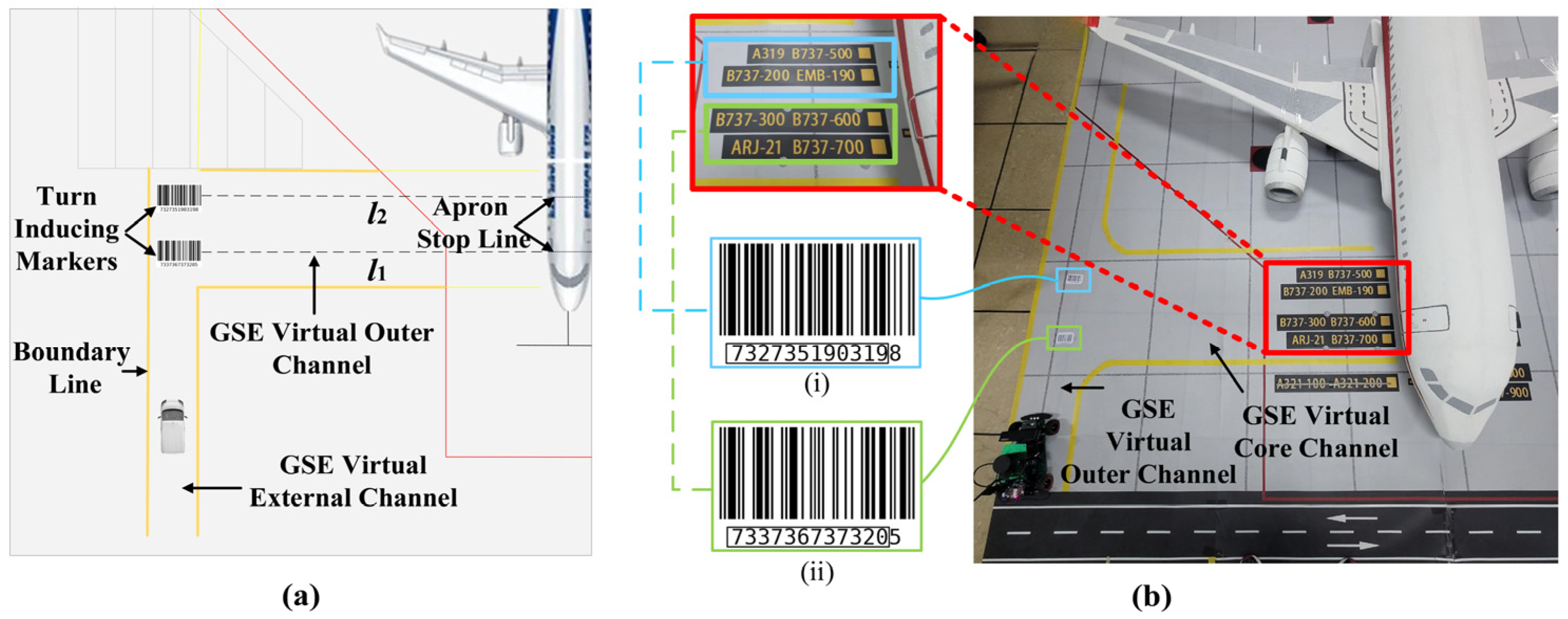
- A novel methodology is introduced for designing virtual channels within an aircraft stand specifically for Unpiloted GSE. This includes the creation of GSE turning induction markers, aimed at optimizing the navigation of GSE towards specific docking positions tailored for different aircraft models.
- We present a perception algorithm tailored for the autonomous navigation of GSE. This algorithm is capable of accurately detecting the boundaries of virtual channels, identifying obstacles, and recognizing docking doors in real time.
- A comprehensive vehicle control algorithm for GSE operating within an aircraft stand is proposed. This encompasses advanced obstacle avoidance strategies and detailed docking control algorithms, ensuring precise and safe docking of the GSE.
1.2. Outline of the Paper
2. Related Work
2.1. Progress in Unpiloted GSE Navigation Research
2.2. Progress in Automatic Docking Technology Research
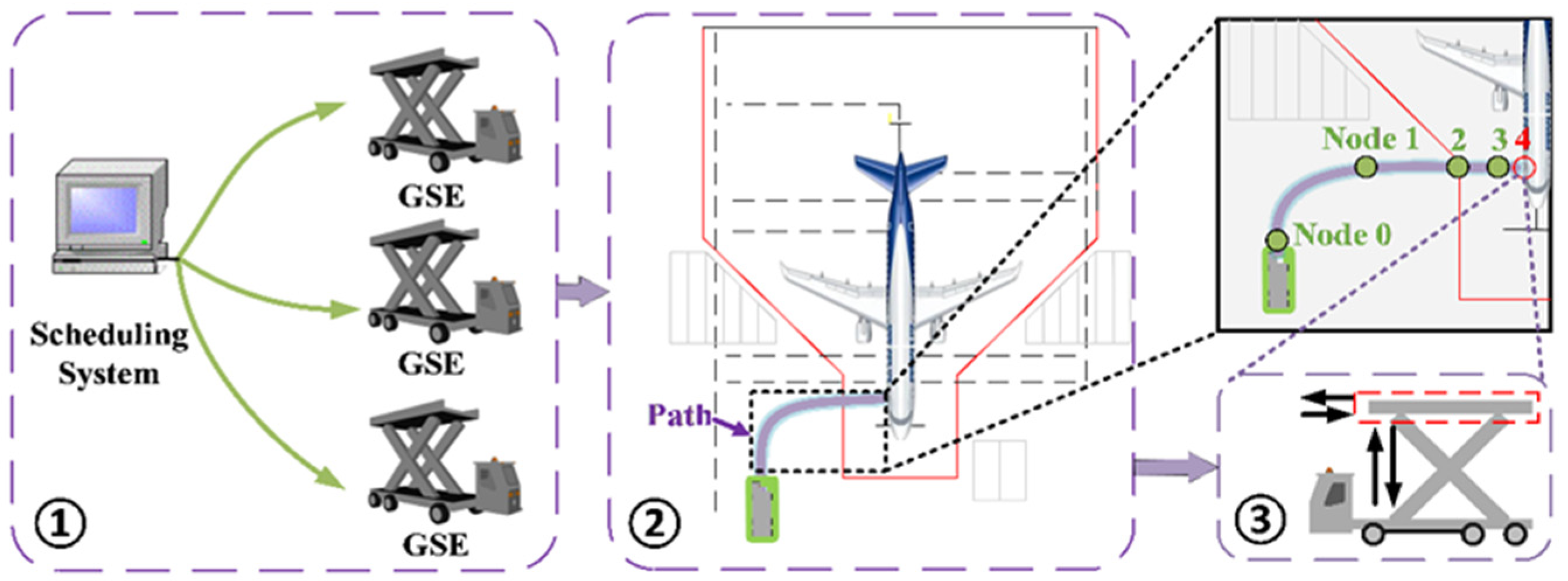
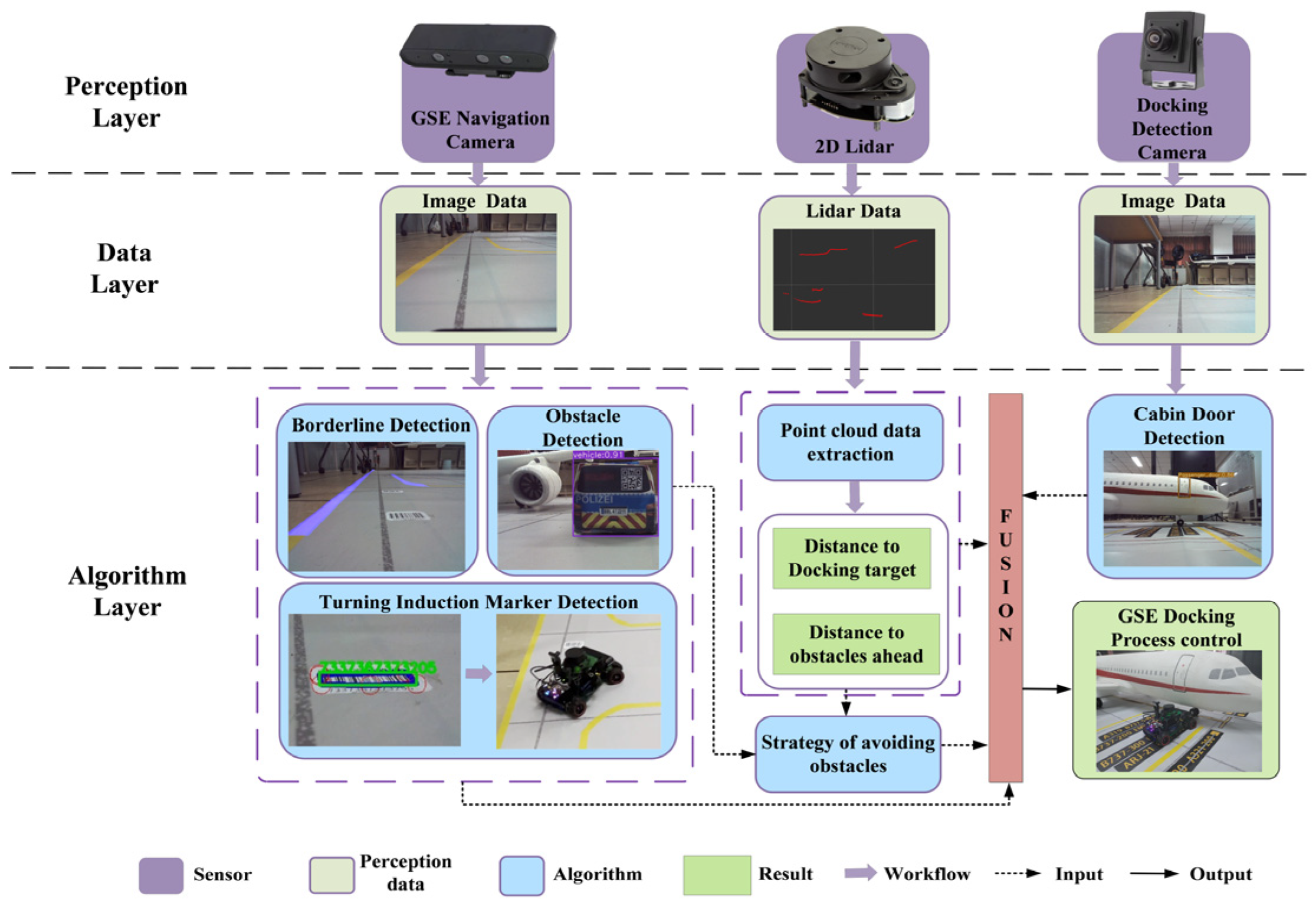
3. Framework of the Detection and Control Algorithm for the Navigation and Cabin Door Docking Process
4. Virtual Channel Layout Method within the Aircraft Stand for Unpiloted GSE
5. Detection Algorithm for Unpiloted GSE
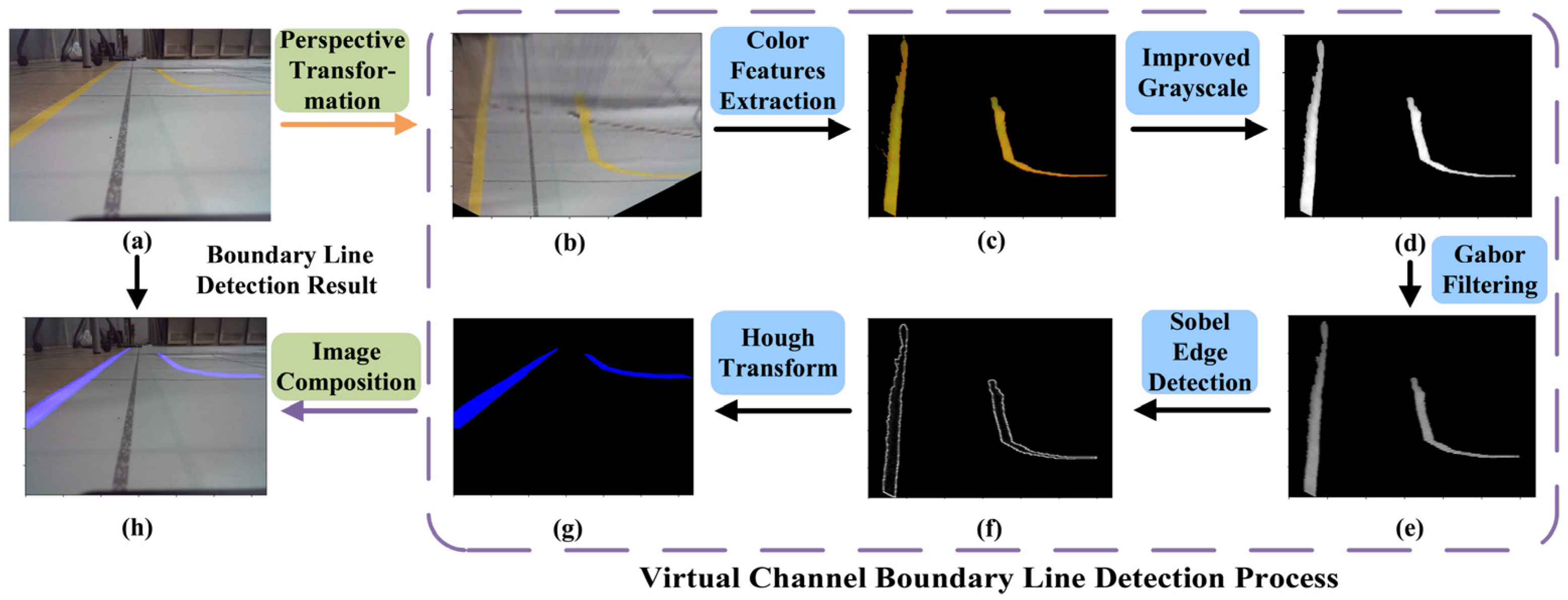
5.1. Virtual Channel Boundary Line Detection within the Aircraft Stand
- (1)
- Perspective Transformation: During the GSE’s navigation within the aircraft stand, the boundary lines captured by the camera appear to converge at a specific distance ahead. This convergence poses challenges for the algorithm in detecting the curvature of the virtual channel boundary lines. To address this, we employ a perspective transformation to convert the original image data into a bird’s-eye view, as demonstrated in Figure 5b.
- (2)
- Color Feature Extraction: Our aim is to isolate the target area of the virtual channel boundary lines and minimize the impact of the color of the virtual channel boundary lines and ground features. In the HSV color space, precise segmentation of the specified color can be achieved. The image after color segmentation is presented in Figure 5c.
- (3)
- Enhanced Grayscale: We utilize an advanced grayscale method to enhance the binarized features of the virtual channel boundary lines. This enhancement facilitates edge extraction and Hough transformation, resulting in improved detection accuracy of the virtual channel boundary lines.
- (4)
- Gabor Filtering: Gabor filtering is a texture analysis technique that combines information from both the spatial and frequency domains [40]. By adjusting the kernel size and selecting the appropriate Gabor filter kernel, we can effectively filter the boundary line image information. The filtered image after transformation is illustrated in Figure 5e.
- (5)
- Sobel Edge Detection and Hough Transformation: Prior to edge detection, we perform morphological closing operations to fill minor holes and smooth the object boundaries in the image. Subsequently, an advanced Sobel operator is employed. Considering the directional characteristics of the virtual channel boundary lines in the images captured by the Unpiloted GSE, we select the Sobel operator in the specific direction to extract diagonal edge features. Post-edge detection, an enhanced Hough transformation is applied to extract straight-line information. By incorporating a constraint factor into the traditional Hough transformation, the identified lines are made continuous, ensuring that the angles of the recognized line segments align with the angle features of the virtual channel boundary lines. The extraction effect is illustrated in Figure 5g.
5.2. Object Detection in the Aircraft Stand Based on Improved YOLO
6. Vehicle Control Algorithm Design for Unpiloted GSE within the Aircraft Stand
6.1. GSE Navigation Control Algorithm
- (1)
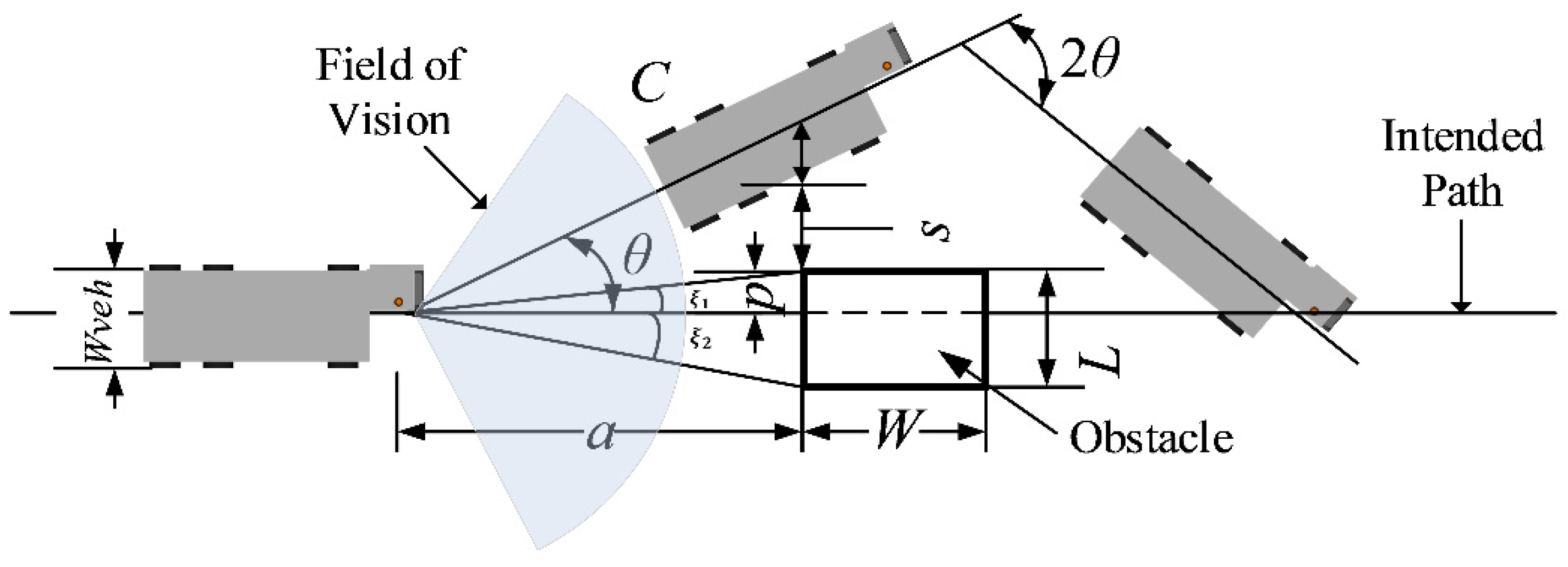
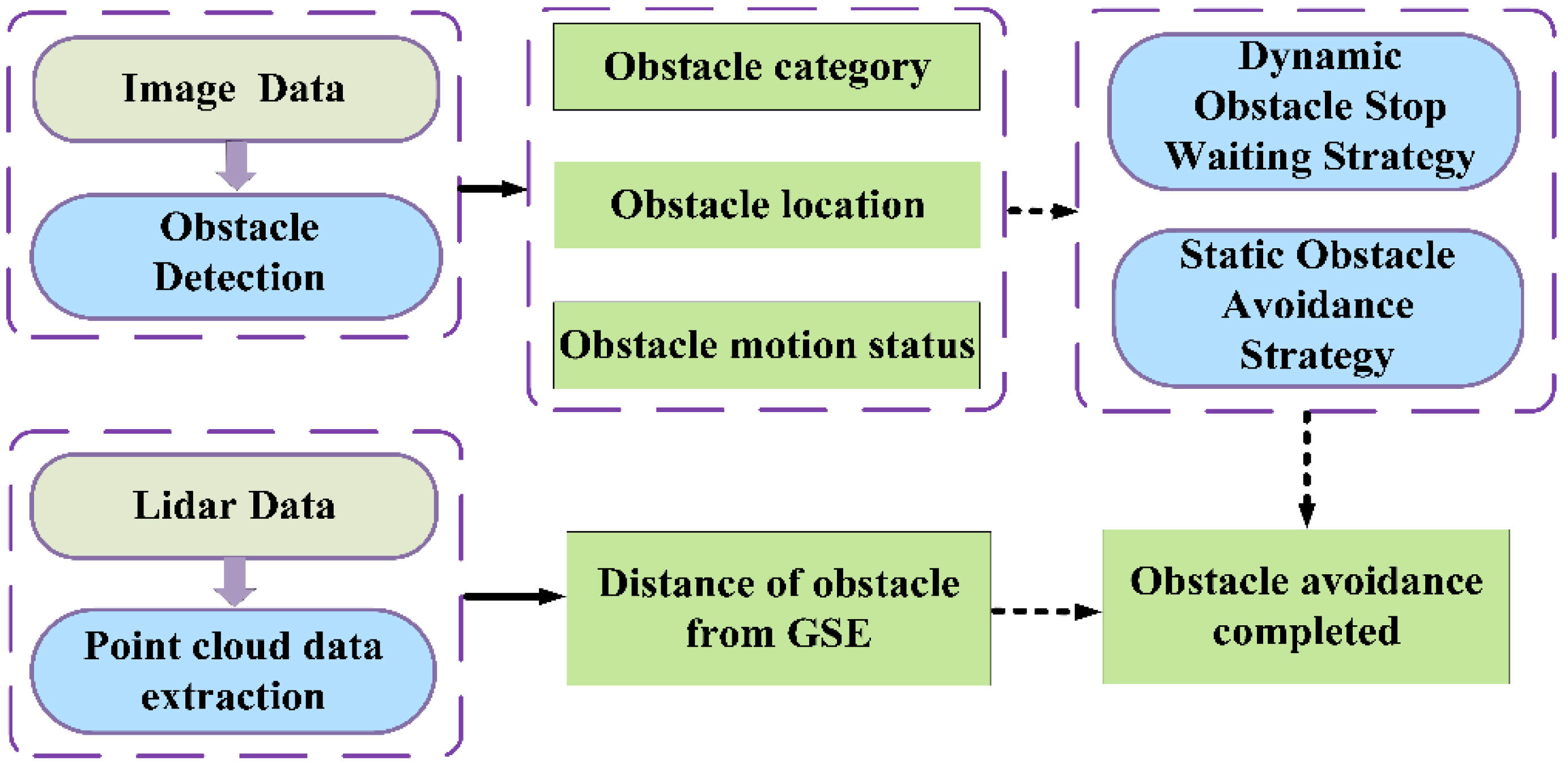
- Obstacle Avoidance Algorithm Design
- (2)
- Dynamic Obstacle Avoidance Strategy
- (3)
- Static Obstacle Avoidance Strategy
6.2. Docking Control Algorithm for Unpiloted GSE
- (1)
- Docking Algorithm Design
- (2)
- Docking Control Strategy
- Node 1—15 m stage: When the Unpiloted GSE is 15 m away from the cabin door, we conduct a brake test. This is to ensure that the GSE can stop in a short time in case of emergencies.
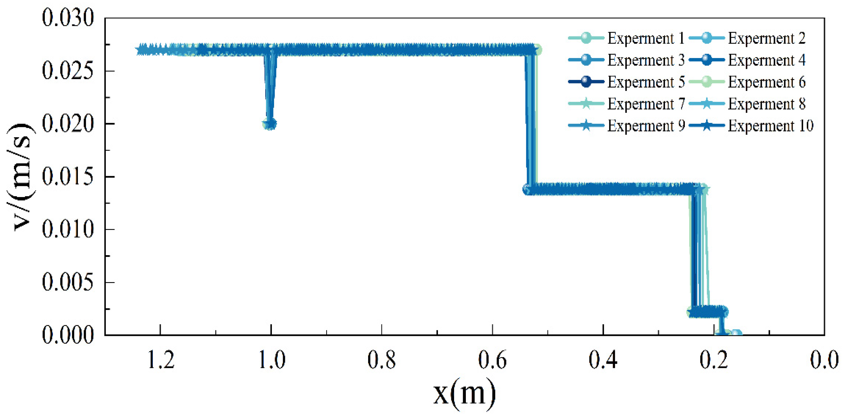
- Node 2—4.50 m stage: When the GSE is 4.50 m away from the cabin door, the GSE first decelerates to 5.00 km/h (1.38 m/s). The main purpose of this stage is to ensure that the GSE has enough time for precise docking when it approaches the cabin door.
- Node 3—0.50 m to 0 m stage: When the GSE is 0.50 m away from the cabin door, the GSE performs a second deceleration to 0.80 km/h (0.22 m/s). During this stage, we ensure that the GSE can dock smoothly and precisely to the cabin door through subtle speed and direction control. Upon arrival, the GSE is brought to a complete stop, marking the end of the docking procedure.
7. Experiment
7.1. Verification of Detection Algorithm for Unpiloted GSE
- (1)
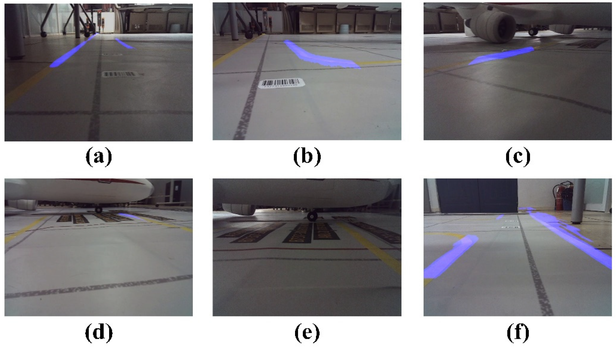
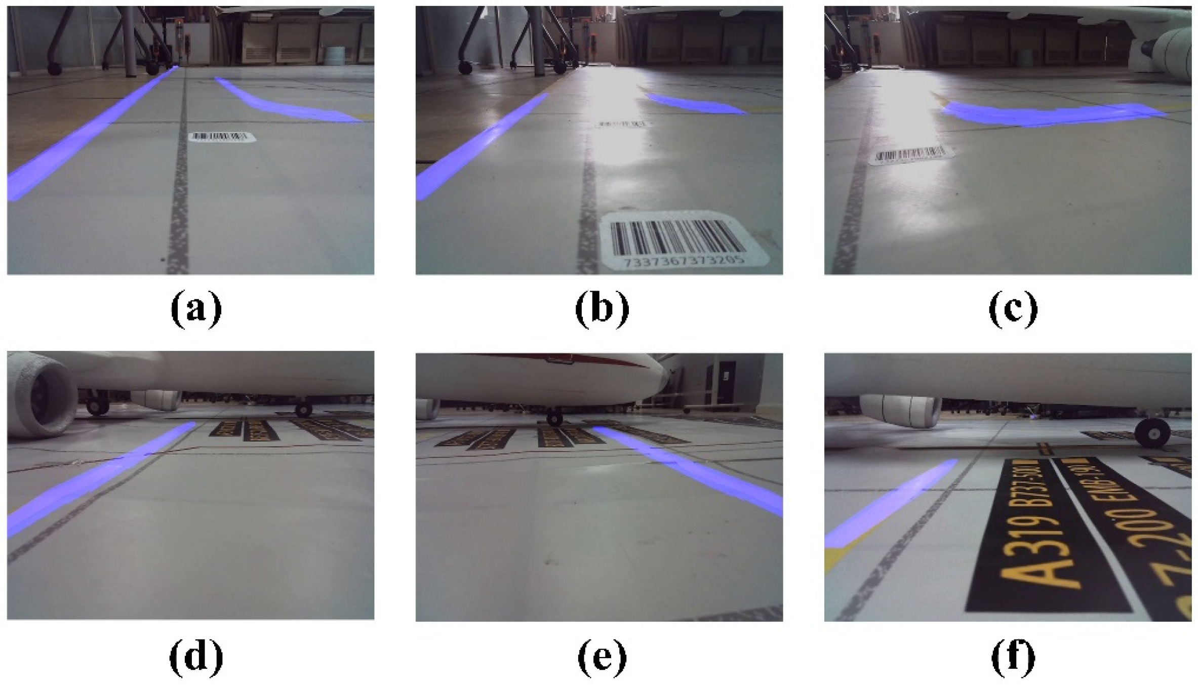
- Experiment on Virtual Channel Boundary Line Detection
- (2)
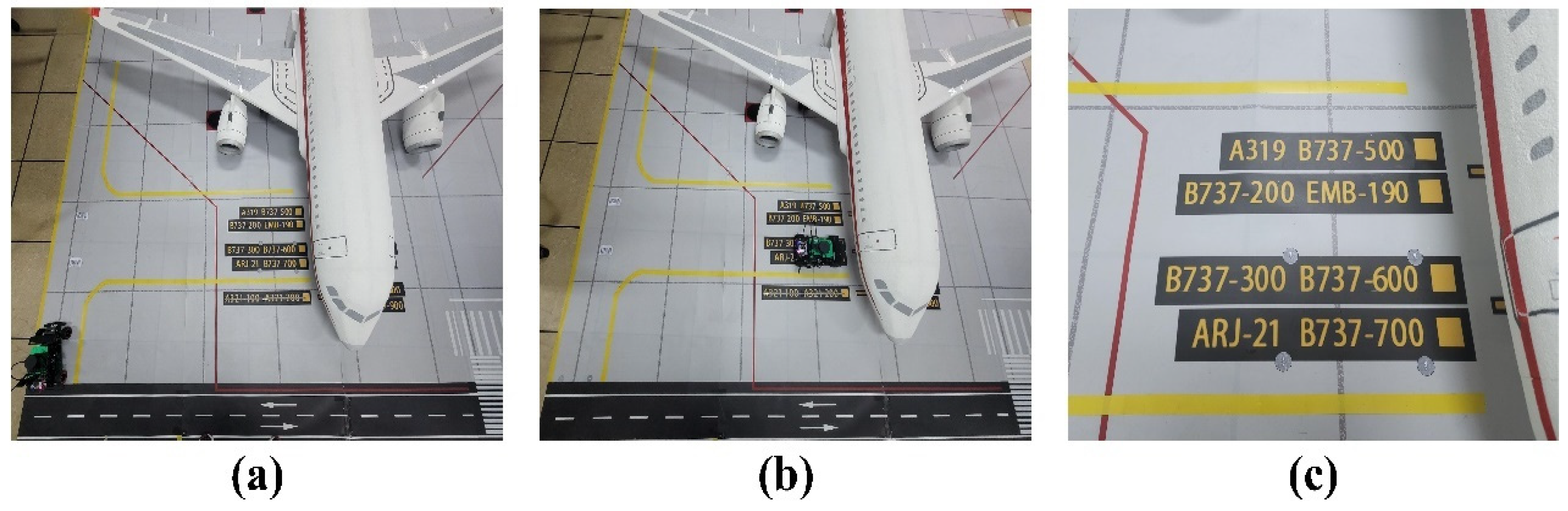
- Experiment on Turning Induction Marker Detection
- (3)
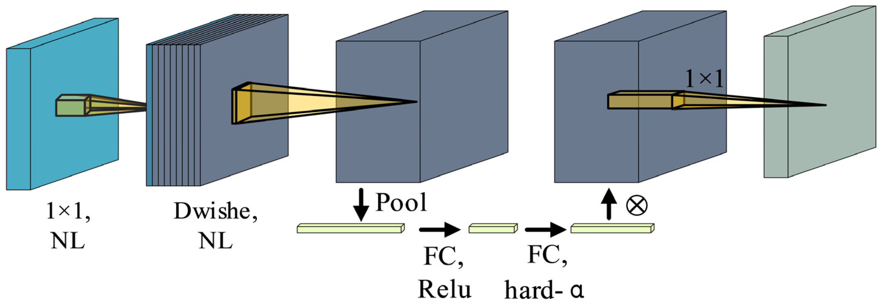
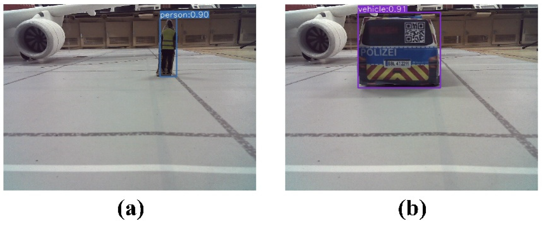
- Experiment on Object Detection in Aircraft Stands Using Improved YOLO
7.2. Verification of Vehicle Control Algorithm for Unpiloted GSE
- (1)
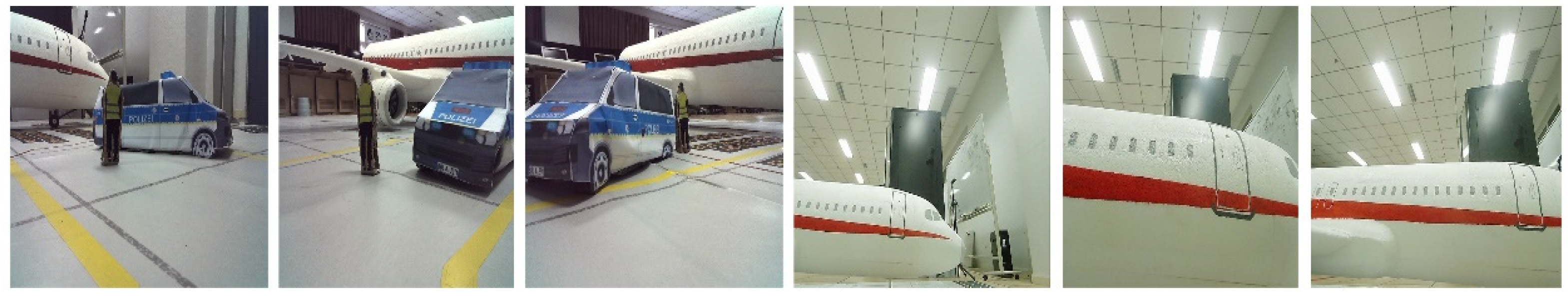
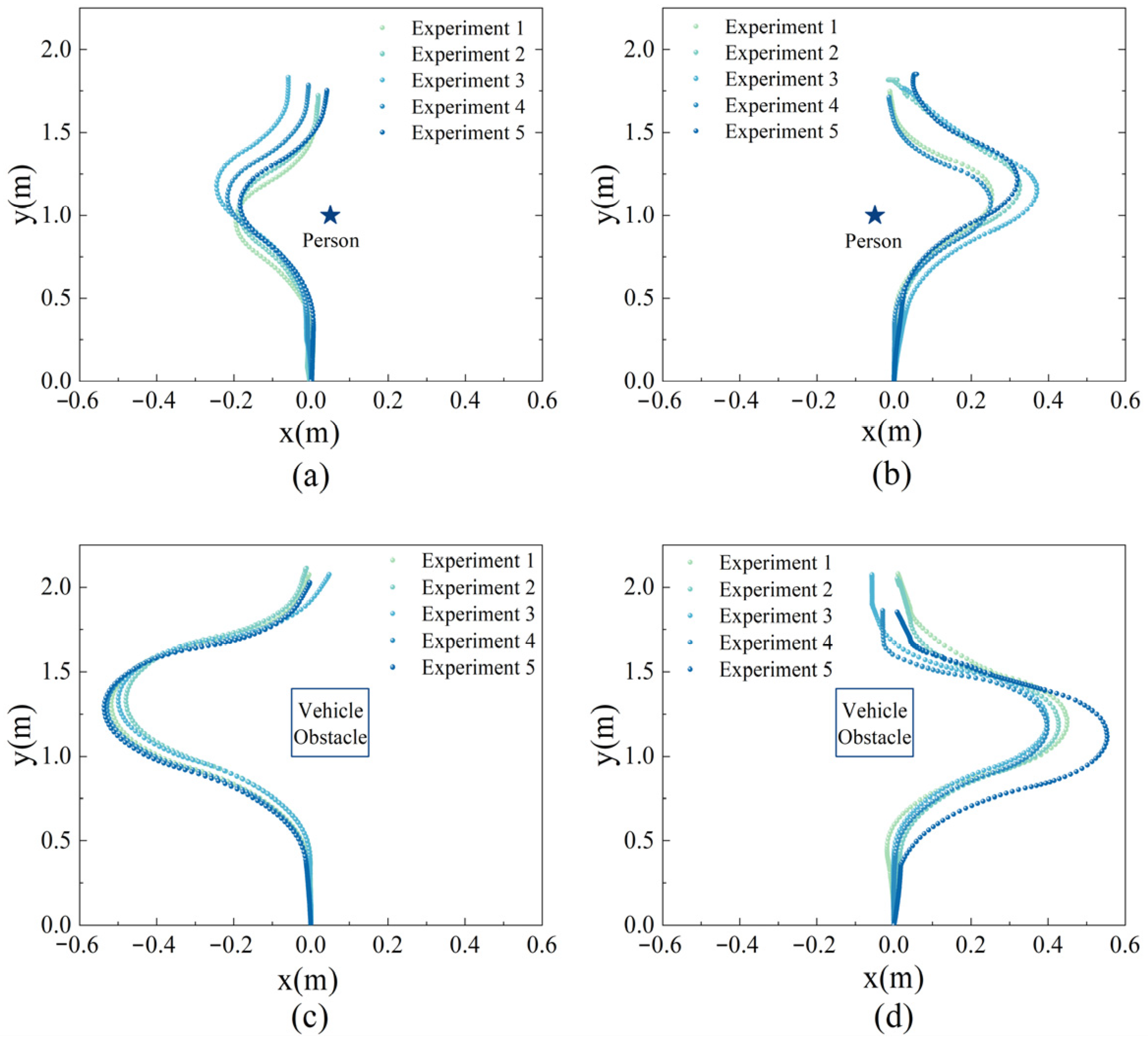
- Verification of GSE Obstacle Avoidance Algorithm
- (2)
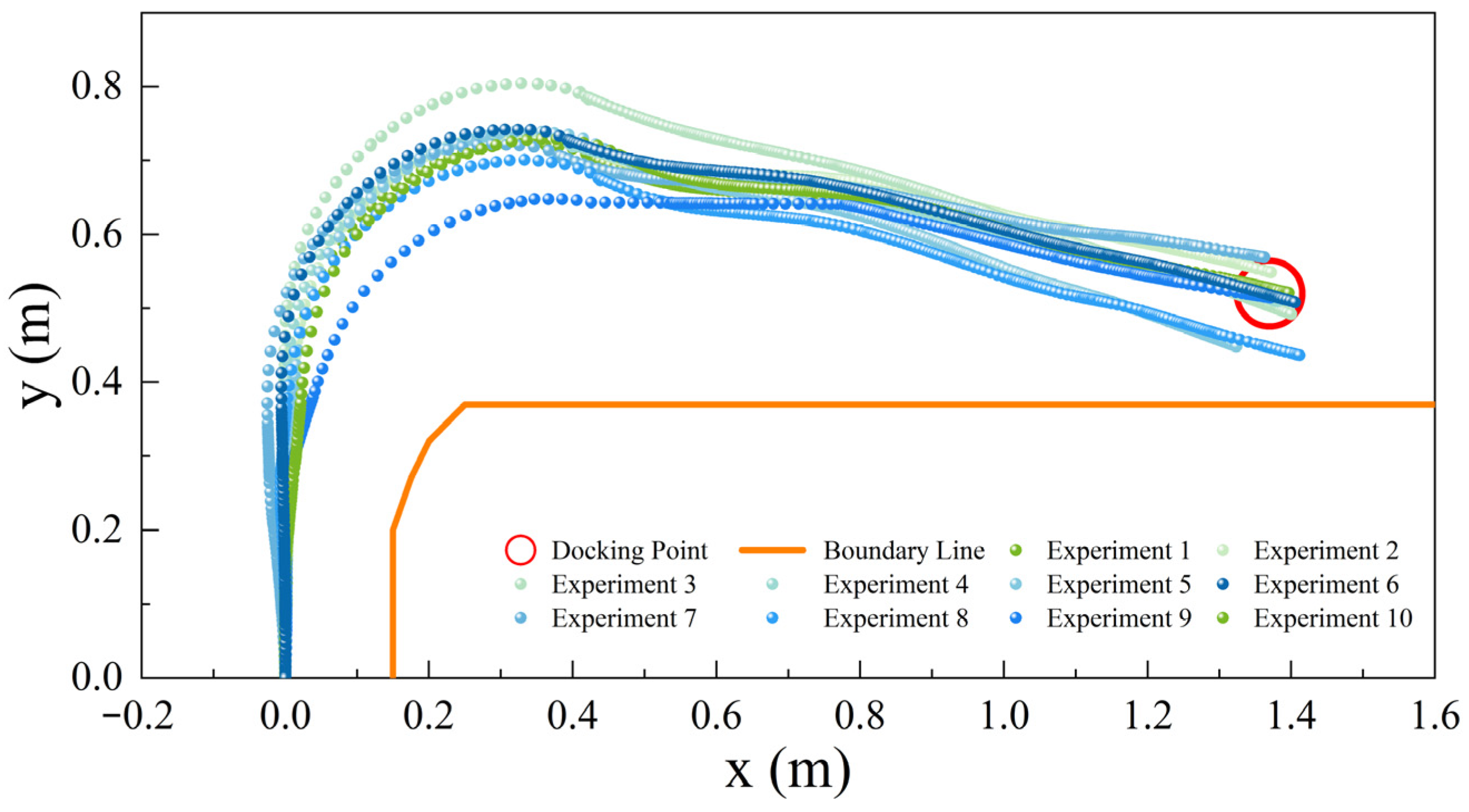
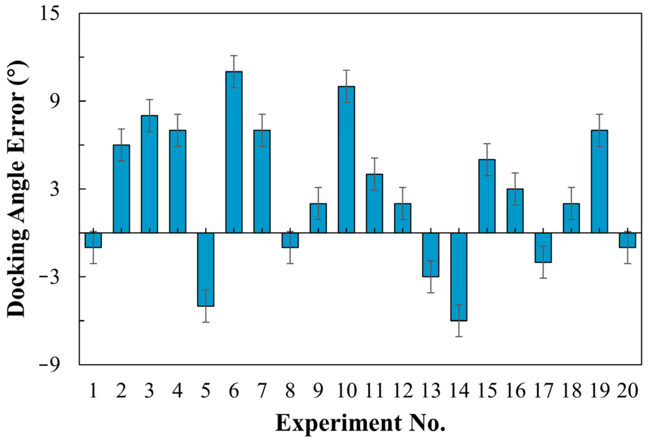
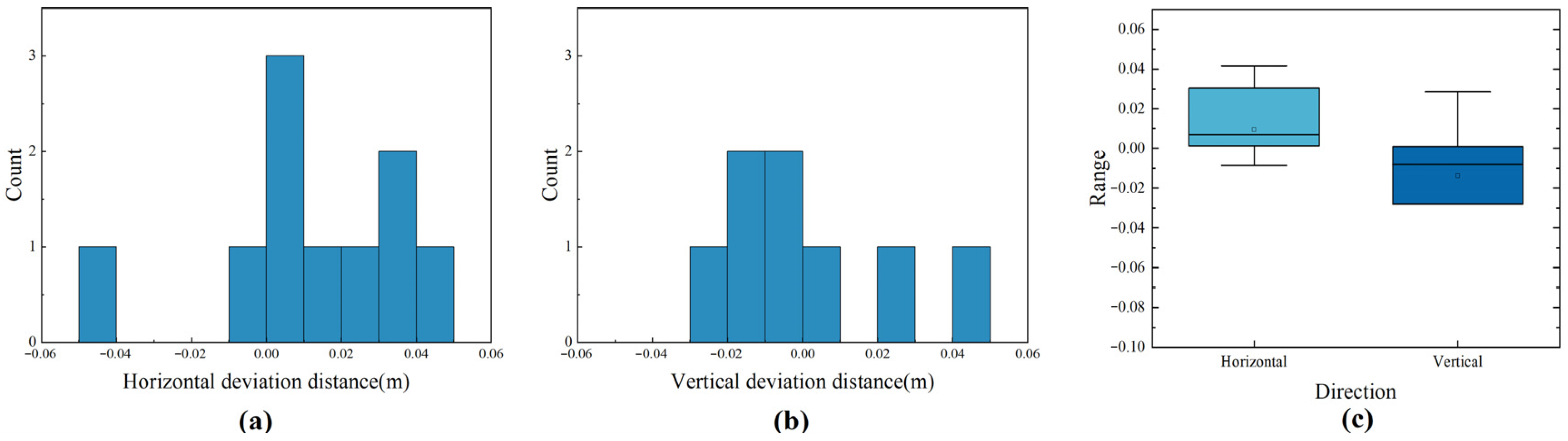
- Verification of GSE Docking Control Algorithm
- During the obstacle avoidance experiment, the turning radius of the vehicle cannot be proportionally reduced, resulting in slower correction of the vehicle’s turning and requiring a longer distance than the actual running distance. However, this issue will be alleviated in real-life scenarios.
- The trajectories of the vehicle in the straight line before turning are not always aligned. This is due to human error in placing the vehicle at the starting position for each experiment, resulting in inconsistencies in the position and angle of the vehicle. Therefore, the vehicle needs to correct its trajectory to the center of the virtual channel after starting. In real situations, this issue will be alleviated.
- As the vehicle lacks a GPS module, it relies solely on an odometer and IMU for positioning, which introduces some errors. In outdoor scenarios, the vehicle may require the addition of a GPS module to assist in correcting the positioning system, thereby obtaining more accurate navigation and positioning results.
8. Conclusions
Author Contributions
Funding
Data Availability Statement
Acknowledgments
Conflicts of Interest
Appendix A

| Model | JIERRUIWEITONG DF-100 |
| Sensor specifications | 1/4 inch |
| Pixel size | 3 µm × 3 µm |
| Highest resolution | 720P |
| Frame rate | 60 |
| Pixel | 1 million |
| Exposure time | 33.33 ms/fps |
| Interface type | USB2.0 |
| Dynamic range | 0.051 lux |
| Model | RPLIDAR A1M8 |
| Measure radius | 0.1–12 m |
| Communication rate | 115,200 bps |
| Sampling frequency | 8 K |
| Scan frequency | 5.5–10 Hz |
| Angular resolution | ≤1° |
| Mechanical dimensions (mm) | 96.8 × 70.3 × 55 |
| CPU | 128-core Maxwell |
| CPU | Quad-core ARM A57 @ 1.43 GHz |
| Memory | 4 GB 64-bit LPDDR4 25.6 GB/s |
| Video Encode | 4K @ 30 | 4× 1080p @ 30 | 9× 720p @ 30 (H.264/H.265) |
| Video Decode | 4K @ 60 | 2× 4K @ 30 | 8× 1080p @ 30 | 18× 720p @ 30 (H.264/H.265) |
| Connectivity | Gigabit Ethernet, M.2 Key E |
| Display | HDMI and display port |
| USB | 4× USB 3.0, USB 2.0 Micro-B |
| Others | GPIO, I2C, I2S, SPI, UART |
| Mechanical | 69 mm × 45 mm, 260-pin edge connector |
References
- Balestrieri, E.; Daponte, P.; De Vito, L.; Lamonaca, F. Sensors and measurements for unmanned systems: An overview. Sensors 2021, 21, 1518. [Google Scholar] [CrossRef] [PubMed]
- Hubbard, S.; Voyles, R.; Souders, D.; Yang, H.; Hart, J.; Brammell, S. Advanced Ground Vehicle Technologies for Airside Operations; The National Academies Press: Washington, DC, USA, 2020. [Google Scholar]
- Huang, S.P. Human Reliability Analysis in Aviation Maintenance by a Bayesian Network Approach. In Proceedings of the 11th International Conference on Structural Safety and Reliability (ICOSSAR2013), New York, NY, USA, 16–20 June 2013. [Google Scholar]
- Kunzi, F. Reduction of Collisions between Aircraft and Surface Vehicles: Conflict Alerting on Airport Surfaces Enabled by Automatic Dependent Surveillance–Broadcast. Transp. Res. Rec. 2013, 2325, 56–62. [Google Scholar] [CrossRef]
- Tomaszewska, J.; Krzysiak, P.; Zieja, M.; Woch, M. Statistical analysis of ground-related incidents at airports. In Proceedings of the 44th International Scientific Congress on Powertrain and Transport Means (EUROPEAN KONES 2018), Czestochowa, Poland, 24–27 September 2018. [Google Scholar]
- CAAC, C.A.A.o.C. Roadmap for the Application of Unmanned Equipment in Airports. 2021. Available online: https://www.ccaonline.cn/zhengfu/zcfg-zhengfu/685373.html (accessed on 20 October 2021).
- Redmon, J.; Divvala, S.; Girshick, R.; Farhadi, A. You Only Look Once: Unified, Real-Time Object Detection. In Proceedings of the Computer Vision & Pattern Recognition, Las Vegas, NV, USA, 27–30 June 2016. [Google Scholar]
- Redmon, J.; Farhadi, A. YOLO9000: Better, Faster, Stronger. In Proceedings of the IEEE Conference on Computer Vision & Pattern Recognition, Honolulu, HI, USA, 21–26 July 2017; pp. 6517–6525. [Google Scholar]
- Jocher, G.; Stoken, A.; Borovec, J.; Chaurasia, A.; Changyu, L.; Hogan, A.; Hajek, J.; Diaconu, L.; Kwon, Y.; Defretin, Y. ultralytics/yolov5: v5. 0-YOLOv5-P6 1280 models, AWS, Supervise. ly and YouTube integrations. Zenodo 2021. [Google Scholar] [CrossRef]
- Kumar, V.; Nakra, B.C.; Mittal, A.P. A Review of Classical and Fuzzy PID Controllers. Int. J. Intell. Control Syst. 2011, 16, 170–181. [Google Scholar]
- Committee, O.-R.A.D. Taxonomy and Definitions for Terms RELATED to Driving Automation Systems for On-Road Motor Vehicles; SAE International: Warrendale, PA, USA, 2021. [Google Scholar]
- Rong, L.J. Introducing Automated Vehicles into Changi Airport’s Landside. Transportation Research Board Committee. 2018. Available online: https://www.straitstimes.com/singapore/transport/ramping-up-automation-at-changi-airport-a-priority-for-next-3-to-5-years-caas-director (accessed on 6 March 2023).
- Phillipson, A. Designing the ‘Airport of the Future’; Aviation Pros: 2019. Available online: https://www.aviationpros.com/airports/consultants/architecture/article/21143854/designing-the-airport-of-the-future (accessed on 13 August 2019).
- Cotton, B. Aurrigo delivers autonomous ‘baggage’ solution for Heathrow. Business Leader News. 25 June 2019. Available online: https://aurrigo.com/aurrigo-delivers-autonomous-baggage-solution-for-heathrow/ (accessed on 25 June 2019).
- Wang, J.; Meng, M.Q.-H. Socially compliant path planning for robotic autonomous luggage trolley collection at airports. Sensors 2019, 19, 2759. [Google Scholar] [CrossRef]
- Wang, S.; Che, Y.; Zhao, H.; Lim, A. Accurate tracking, collision detection, and optimal scheduling of airport ground support equipment. IEEE Internet Things J. 2020, 8, 572–584. [Google Scholar] [CrossRef]
- Donadio, F.; Frejaville, J.; Larnier, S.; Vetault, S. Artificial Intelligence and Collaborative Robot to Improve Airport Operations; Springer: Cham, Switzerland, 2018; pp. 973–986. [Google Scholar]
- Jovančević, I.; Viana, I.; Orteu, J.-J.; Sentenac, T.; Larnier, S. Matching CAD model and image features for robot navigation and inspection of an aircraft. In Proceedings of the International Conference on Pattern Recognition Applications & Methods, Roma, Italy, 24–26 February 2016. [Google Scholar]
- Elrayes, A.; Ali, M.H.; Zakaria, A.; Ismail, M.H. Smart airport foreign object debris detection rover using LiDAR technology. Internet Things 2019, 5, 1–11. [Google Scholar] [CrossRef]
- Kim, C.-H.; Jeong, K.-M.; Jeong, T.-W. Semi-autonomous navigation of an unmanned ground vehicle for bird expellant in an airport. In Proceedings of the 2012 12th International Conference on Control, Automation and Systems, Jeju, Republic of Korea, 17–21 October 2012; pp. 2063–2067. [Google Scholar]
- Lee, S.; Seo, S.-W. Sensor fusion for aircraft detection at airport ramps using conditional random fields. IEEE Trans. Intell. Transp. Syst. 2022, 23, 18100–18112. [Google Scholar] [CrossRef]
- Anderberg, N.-E. Method for Automated Docking of a Passenger Bridge or a Goods Handling Bridge to a Door of an Aircraft. U.S. Patent US20090217468A1, 3 September 2009. [Google Scholar]
- Glatfelter, J.W.; Laughlin, B.D. System and Method for Automated Deployment of a Passenger Boarding Bridge. U.S. Patent No 10,519,614, 31 December 2019. [Google Scholar]
- Futterlieb, M.; Cadenat, V.; Sentenac, T. A navigational framework combining Visual Servoing and spiral obstacle avoidance techniques. In Proceedings of the 2014 11th International Conference on Informatics in Control, Automation and Robotics (ICINCO), Vienna, Austria, 1–3 September 2014; pp. 57–64. [Google Scholar]
- Perez, M.P.; Juliana, H.M.G. Método Para Colocar una Pasarela de Embarque Para Pasajeros en un Avión. ES2706886T3, 1 April 2019. [Google Scholar]
- Liu, X.; Deng, Z. Segmentation of Drivable Road Using Deep Fully Convolutional Residual Network with Pyramid Pooling. Cogn. Comput. 2018, 10, 272–281. [Google Scholar] [CrossRef]
- Neven, D.; De Brabandere, B.; Georgoulis, S.; Proesmans, M.; Van Gool, L. Towards End-to-End Lane Detection: An Instance Segmentation Approach. IEEE Embed. Syst. Lett. 2018, 2018, 286–291. [Google Scholar] [CrossRef]
- Pizzati, F.; García, F. Enhanced free space detection in multiple lanes based on single CNN with scene identification. In Proceedings of the 2019 IEEE Intelligent Vehicles Symposium (IV), Paris, France, 9–12 June 2019. [Google Scholar]
- Satzoda, R.K.; Sathyanarayana, S.; Srikanthan, T. Hierarchical Additive Hough Transform for Lane Detection. IEEE Embed. Syst. Lett. 2010, 2, 23–26. [Google Scholar] [CrossRef]
- Zhang, G.; Zheng, N.; Cui, C.; Yuzhen, Y.; Zejian, Y. An efficient road detection method in noisy urban environment. In Proceedings of the 2009 IEEE Intelligent Vehicles Symposium, Xi’an, China, 3–5 June 2009; pp. 556–561. [Google Scholar]
- Chen, X.; Ma, H.; Wan, J.; Li, B.; Xia, T. Multi-View 3D Object Detection Network for Autonomous Driving. In Proceedings of the 2017 IEEE Conference on Computer Vision and Pattern Recognition (CVPR), Honolulu, HI, USA, 21–26 July 2017. [Google Scholar]
- Geng, K.; Dong, G.; Yin, G.; Hu, J. Deep Dual-Modal Traffic Objects Instance Segmentation Method Using Camera and LIDAR Data for Autonomous Driving. Remote Sens. 2020, 12, 3274. [Google Scholar] [CrossRef]
- Ku, J.; Mozifian, M.; Lee, J.; Harakeh, A.; Waslander, S.L. Joint 3D Proposal Generation and Object Detection from View Aggregation. In Proceedings of the 2018 IEEE/RSJ International Conference on Intelligent Robots and Systems (IROS), Madrid, Spain, 1–5 October 2018; pp. 1–8. [Google Scholar]
- Wu, B.; Wan, A.; Iandola, F.; Jin, P.H.; Keutzer, K. SqueezeDet: Unified, Small, Low Power Fully Convolutional Neural Networks for Real-Time Object Detection for Autonomous Driving. IEEE Embed. Syst. Lett. 2017, 60, 129–137. [Google Scholar] [CrossRef]
- Zhang, Y.; Liu, K.; Bao, H.; Zheng, Y.; Yang, Y. PMPF: Point-Cloud Multiple-Pixel Fusion-Based 3D Object Detection for Autonomous Driving. Remote Sens. 2023, 15, 1580. [Google Scholar] [CrossRef]
- Hubmann, C.; Schulz, J.; Becker, M.; Althoff, D.; Stiller, C. Automated Driving in Uncertain Environments: Planning with Interaction and Uncertain Maneuver Prediction. IEEE Trans. Intell. Veh. 2018, 3, 5–17. [Google Scholar] [CrossRef]
- Okumura, B.; James, M.; Kanzawa, Y.; Derry, M.; Sakai, K.; Nishi, T.; Prokhorov, D. Challenges in Perception and Decision Making for Intelligent Automotive Vehicles: A Case Study. IEEE Trans. Intell. Veh. 2016, 1, 20–32. [Google Scholar] [CrossRef]
- Alonso Tabares, D.; Mora-Camino, F. Aircraft ground handling: Analysis for automation. In Proceedings of the 17th AIAA Aviation Technology, Integration, and Operations Conference, Denver, CO, USA, 5–9 June 2017; p. 3425. [Google Scholar]
- Zhang, Z. A flexible new technique for camera calibration. IEEE Trans. Pattern Anal. Mach. Intell. 2000, 22, 1330–1334. [Google Scholar] [CrossRef]
- Gonzalez, R.C.; Woods, R.E. Digital Image Processing, 2nd ed.; Springer Science & Business Media: Berlin/Heidelberg, Germany, 2002. [Google Scholar]
- Howard, A.; Sandler, M.; Chen, B.; Wang, W.; Chen, L.C.; Tan, M.; Chu, G.; Vasudevan, V.; Zhu, Y.; Pang, R.; et al. Searching for MobileNetV3. In Proceedings of the 2019 IEEE/CVF International Conference on Computer Vision (ICCV), Seoul, Republic of Korea, 27 October–2 November 2019; pp. 1314–1324. [Google Scholar]
- Pentland, A.; Liu, A. Modeling and prediction of human behavior. Neural Comput. 1999, 11, 229–242. [Google Scholar] [CrossRef]
- López, A.; Serrat, J.; Cañero, C.; Lumbreras, F.; Graf, T. Robust lane markings detection and road geometry computation. Int. J. Automot. Technol. 2010, 11, 395–407. [Google Scholar] [CrossRef]
- International Civil Aviation Organization. Annex 14—Aerodromes (ICAO Doc 9137-AN/898); ICAO: Montreal, NA, Canada, 2018. [Google Scholar]
- Wang, Z.; Delahaye, D.; Farges, J.-L.; Alam, S. Route network design in low-altitude airspace for future urban air mobility operations A case study of urban airspace of Singapore. In Proceedings of the International Conference on Research in Air Transportation (ICRAT 2020), Tampa, FL, USA, 26–29 June 2020. [Google Scholar]
- Wang, Z.; Delahaye, D.; Farges, J.-L.; Alam, S. A quasi-dynamic air traffic assignment model for mitigating air traffic complexity and congestion for high-density UAM operations. Transp. Res. Part C Emerg. 2023, 154, 104279. [Google Scholar] [CrossRef]
- Qiong, W.; Shuai, S.; Ziyang, W.; Qiang, F.; Pingyi, F.; Cui, Z. Towards V2I age-aware fairness access: A DQN based intelligent vehicular node training and test method. Chin. J. Electron. 2023, 32, 1230–1244. [Google Scholar] [CrossRef]


| HSV Parameter | Minimum Value | Title 3 |
|---|---|---|
| H | 23 | 180 |
| S | 104 | 255 |
| V | 44 | 255 |
| Type | Results |
|---|---|
| Missed detection (minor) | 4 cases, 51 frames |
| False detection | 1 case, 26 frames |
| Detection failed | 3 cases, 30 frames |
| GFlops | Parameters | |
|---|---|---|
| YOLOv5s | 16.5 | 7,068,936 |
| YOLOv5s-MobileNetV3 | 2.3 | 1,382,846 |
Disclaimer/Publisher’s Note: The statements, opinions and data contained in all publications are solely those of the individual author(s) and contributor(s) and not of MDPI and/or the editor(s). MDPI and/or the editor(s) disclaim responsibility for any injury to people or property resulting from any ideas, methods, instructions or products referred to in the content. |
© 2023 by the authors. Licensee MDPI, Basel, Switzerland. This article is an open access article distributed under the terms and conditions of the Creative Commons Attribution (CC BY) license (https://creativecommons.org/licenses/by/4.0/).
Share and Cite
Zhang, T.; Zhang, Z.; Zhu, X. Detection and Control Framework for Unpiloted Ground Support Equipment within the Aircraft Stand. Sensors 2024, 24, 205. https://doi.org/10.3390/s24010205
Zhang T, Zhang Z, Zhu X. Detection and Control Framework for Unpiloted Ground Support Equipment within the Aircraft Stand. Sensors. 2024; 24(1):205. https://doi.org/10.3390/s24010205
Chicago/Turabian StyleZhang, Tianxiong, Zhiqiang Zhang, and Xinping Zhu. 2024. "Detection and Control Framework for Unpiloted Ground Support Equipment within the Aircraft Stand" Sensors 24, no. 1: 205. https://doi.org/10.3390/s24010205
APA StyleZhang, T., Zhang, Z., & Zhu, X. (2024). Detection and Control Framework for Unpiloted Ground Support Equipment within the Aircraft Stand. Sensors, 24(1), 205. https://doi.org/10.3390/s24010205