You are currently viewing a new version of our website. To view the old version click .
Sensors
  • Article
  • Open Access

27 December 2023

Ultra-Lightweight Fast Anomaly Detectors for Industrial Applications

,
and
1
KSM Vision sp. z o.o., 01-142 Warsaw, Poland
2
Institute of Automatic Control and Robotics, Warsaw University of Technology, 02-525 Warsaw, Poland
*
Author to whom correspondence should be addressed.
This article belongs to the Section Industrial Sensors

Abstract

Quality inspection in the pharmaceutical and food industry is crucial to ensure that products are safe for the customers. Among the properties that are controlled in the production process are chemical composition, the content of the active substances, and visual appearance. Although the latter may not influence the product’s properties, it lowers customers’ confidence in drugs or food and affects brand perception. The visual appearance of the consumer goods is typically inspected during the packaging process using machine vision quality inspection systems. In line with the current trends, the processing of the images is often supported with deep neural networks, which increases the accuracy of detection and classification of faults. Solutions based on AI are best suited to production lines with a limited number of formats or highly repeatable production. In the case where formats differ significantly from each other and are often being changed, a quality inspection system has to enable fast training. In this paper, we present a fast method for image anomaly detection that is used in high-speed production lines. The proposed method meets these requirements: It is easy and fast to train, even on devices with limited computing power. The inference time for each production sample is sufficient for real-time scenarios. Additionally, the ultra-lightweight algorithm can be easily adapted to different products and different market segments. In this work, we present the results of our algorithm on three different real production data gathered from food and pharmaceutical industries.

1. Introduction

Pharmaceutical and food manufacturers must comply with restrictive norms to ensure the highest quality standards. These standards apply to both production and packaging. The delivery of an incorrectly sealed product or a product in damaged packaging can result in complaints and sometimes the withdrawal of the entire product series from the market. Consequently, this means financial losses for the manufacturer.
Machine vision technologies are increasingly taking over traditional manual or visual inspection methods, becoming the standard in the pharmaceutical and food manufacturing industries. These machine vision solutions eliminate the need for direct contact with the inspected product, guaranteeing consistent and repeatable results. Moreover, they are specifically designed to function efficiently in high-speed production lines. The incorporation of algorithms rooted in deep neural networks further expands the scope of automatic quality control applications.
The problem with using standard, widespread solutions arises in contract manufacturing when different formats are produced on a single production line (or in a single production run). Defect detection models need to be adjusted (retrained) for each new format, which, when formats change two or three times a day, can result in long production downtime and system start-up errors. An example of the mentioned production type is packaging pharmaceuticals in blisters or bottle capping in the bottling industry. The diversity of tablets, capsules, bottles, and caps makes the fault detection algorithm cumbersome and time-consuming. This creates the need to use fast-to-operate and quick-to-set models for defect detection.
To address all of the objectives mentioned above, a fast, universal, adaptive, and ultra-lightweight anomaly detector was created. The effectiveness and adaptability of the proposed solution are demonstrated in the example of quality control of drugs in blisters, quality control of liquid packaging closures, and quality control of foreign bodies in food packaging using X-ray imaging.
This paper is organized as follows: Following the introduction is the section discussing related works. In Section 3, the design of our fast and lightweight system is presented with a detailed description of its parts: feature extractor, feature preprocessing, anomaly detector, and training procedure. Section 4 contains our experimental results compared with other anomaly detection models. Then, a use case with X-ray images is presented. This article concludes with a summary and future work descriptions.

3. The Methodology

3.1. System Overview

Our anomaly detection system consists of three components: feature extractor, feature preprocessing block, and autoencoder. The architecture of our system is shown in Figure 1.
Figure 1. Our anomaly detection system’s main components.
The feature extractor is responsible for capturing relevant information from the input image. We use a pretrained CNN to obtain well-generalized features. The next step is feature scaling, which standardizes the extracted features, ensuring they are on the same scale. Scaled features are passed to the autoencoder, which creates the reconstruction of input features. Finally, reconstruction loss is calculated as the difference between input and reconstruction features. The value of reconstruction loss is treated as an anomaly score. The training of our system is limited to setting the parameters of the feature scaler and training the autoencoder, which enables fast training on edge devices with limited computing power.

3.2. Features Extraction

The fundamental objective of the feature extractor is extracting pertinent information from the input image. Our system uses a CNN architecture MobileNetV2 [52] as a backbone. The network’s input shape is dynamically determined internally by our system, an adaptive process aligning the architecture with the original dimensions of the input images. The input dimensions of the neural network are determined from a predefined set of options. These options were prepared based on the most common image shapes existing in our computer vision systems. This adaptability is integral to accommodating diverse image sizes and resolutions encountered in real-world applications. We leverage a pretrained instantiation of MobileNetV2, initially trained on the ImageNet dataset [53] with the width multiplier parameter set to 1.
Input images of the feature extractor network have to be preprocessed so the features can be extracted properly. For MobileNetV2, the only required preprocessing is image scaling into the range [0.0, 1.0].
MobileNetV2’s primary objective is a classification task; to harness its feature extraction prowess, we discard the final layers of the model. Instead, we select the “block_15_add” layer within the network as the output layer.

3.3. Feature Preprocessing Block

In the context of our study, it is imperative to preprocess extracted features to align them with the proposed autoencoder architecture. Assuming an input shape of (224, 224, 3) for the CNN backbone, the features extracted from it are initially organized in a 7 × 7 × 160 tensor structure. This tensor retains spatial information, which, at this particular stage, is not necessary. Consequently, a flattening operation is performed, transforming the tensor into a vector with a dimensionality of 7840.
The next step is feature normalization, which ensures that all features have the same scale and will have a comparable impact on the autoencoder’s predictions. We use min–max normalization, rescaling each feature to the 0–1 range. Minimum and maximum values for each feature are dynamically computed during the training phase of the system. These values are then used during the inference phase to ensure that new sample’s features are comparable with the training ones.

3.4. Autoencoder

The proposed autoencoder architecture is a fully connected neural network with batch normalization layers and one dropout layer. The autoencoder was implemented in TensorFlow with the use of Keras layers. The final architecture of the autoencoder is a result of experiments on diverse datasets from different products and different market segments. This empirical approach ensures the adaptability and robustness of the final autoencoder design, substantiating its efficacy across a broad range of applications and domains. The structure of the autoencoder is presented in Table 1.
Table 1. Autoencoder architecture.
Reconstruction error is calculated as the difference between input features and the autoencoder output. The reconstruction error is calculated via the application of the mean squared error (MSE) metric. Following the reconstruction process, the reconstruction error undergoes polynomial transformation. The coefficients of the polynomial function are computed to align with a manually devised function designed to convert reconstruction error values into a representation that is more comprehensible to human interpretation. Subsequently, these transformed values are constrained within the interval [0, 0.99], resulting in the derivation of an anomaly score. In the majority of practical scenarios, it is observed that normal samples exhibit anomaly scores that tend to be lower than 0.25 after undergoing these sequential transformations.
The system’s input image is classified as abnormal if its anomaly score is larger than the threshold value. The threshold is set automatically based on the values of anomaly scores of training samples but can be fine-tuned manually by a human operator.

3.5. Training

The training of our system consists of two stages. In the first stage, all correct training images are preprocessed and then passed through the feature extractor. Minimum and maximum values for each feature are calculated and set as parameters for the min–max scaler, and based on these parameters, training features are scaled. The same configuration of the min–max scaler will be used on the new sample inference. Scaled training features are used to train the autoencoder network.
In the second stage, we train the autoencoder for 50 epochs. We use Adamax with a learning rate set to 0.001 as optimizer and MSE as loss function. the metric used for model evaluation is also MSE. Using the same metric for training and calculating reconstruction error ensures that the autoencoder will try to minimize anomaly scores on training samples.
In the realm of industrial applications, our system undergoes training, employing a dataset comprising no fewer than 200 images. The features extracted from these data enable the autoencoder to learn the intricate patterns and nuances present within the dataset of nonanomalous samples, thereby enhancing its capacity for discernment and classification in real-world industrial scenario.

4. The Experiments

4.1. Datasets

We evaluated our method on three datasets: one public dataset and two datasets gathered by vision systems installed on industrial production lines.
As a public dataset, we chose MVTec anomaly detection dataset [54,55], which focuses on industrial inspection. MVTec AD contains over 5000 images divided into 15 categories. Each category has its own training set with nonanomalous samples and a test set containing both anomalous and nonanomalous samples.
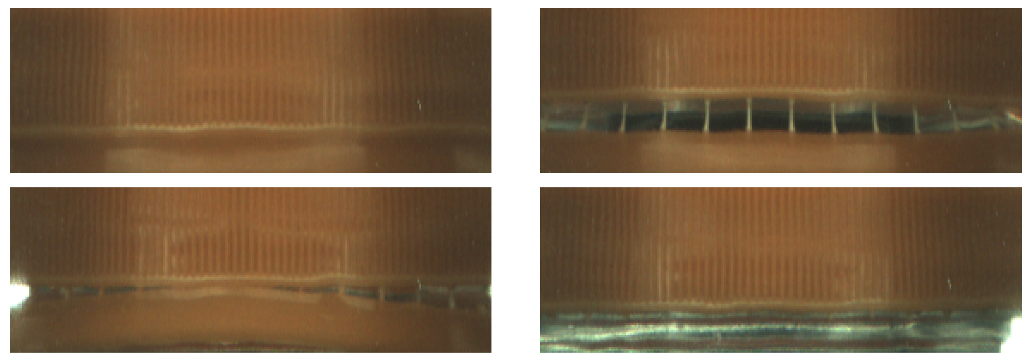
Two other datasets contain data collected on different production lines from different manufacturing domains: pharmaceutical and food markets. The first dataset contains images gathered by our vision system installed on machine for packaging pharmaceutical pills in blisters. The images of single pills are cropped from a full image based on predefined regions. Across the machines integrated with our optical quality control system, a diverse array of pills and capsules are packed into blisters, varying in terms of size, geometry, and coloration (Figure 2). Our anomaly detection system works for all pill–blister combinations. Images in the second dataset were acquired on the beverage production line. Our quality control system detects faults in bottle caps; a 360-degree image of the bottle cap is captured with a single camera. The caps, which are visible on mirrors, are remapped to rectangular images. See Figure 3 and Figure 4. The sizes and colors of controlled caps differ for different beverages, but all of them are controlled with our anomaly detection system (Figure 1). Both datasets preserve the same test and train set structure as each MVTec AD category.
Figure 2. Images gathered by vision system installed on a machine for packaging pharmaceutical pills in blisters.
Figure 3. Images gathered by vision system installed on beverage production line. A 360-degree image of the bottle cap is obtained with a single camera with the use of mirrors.
Figure 4. Sample normal (top left) and anomalous images from bottle cap dataset. Images are rectified (unwrapped) from Figure 3.
The training set of the pills dataset contains 350 RGB images of white oblong pills on an aluminum background. All images have the shape (100, 210, 3). The test set contains 250 nonanomalous samples and 224 defective samples. Abnormal samples have different types of defects: scratches, cracks, improper pill orientation, missing part of the pill, or extra pill elements.
The bottle cap dataset consists of data from Inspect360+ visual inspection systems. Caps image are gathered with a single camera and transformed with the calibration procedure described in [56]. The training set contains 243 RGB images with the shape (280, 96, 3). The test set contains 160 normal and 132 abnormal images with defects: broken inviolability ring, absence of cap, and inclined cap.
Samples from pills and bottle cap datasets are shown in Figure 4 and Figure 5.
Figure 5. Sample normal (two most left) and anomalous images from pills dataset.

4.2. Anomaly Detection Models

We compare our solution with FastFLow [57], EfficientAD [58], Deep Feature Kernel Density Estimation (DFKDE), DFM [59], PaDiM [60], and PathCore [24]. We used implementations provided by anomalib library [61] with default parameters. For FastFlow, we used a ResNet18 backbone, set the number of flow steps to 8, and only used 3 × 3 convolutional layers in flow steps. A small version of EfficentAD was used—EfficientAD-S with 384 channels on the output of the teacher network. For DFKDE, a ResNet18 was used as the backbone, and the number of PCA components was set to 16. For DFM, we used a ResNet50 backbone and set PCA to retain 97% of the original data variance. For PaDiM, we also used the ResNet18 backbone. We used the PatchCore-10% version of PatchCore algorithm with WideResNet50_2 used as the backbone. For all models, images were resized to (256, 256), and further cropping was omitted.

4.3. Metrics and Experimental Setup

For the evaluation of models, we selected two metrics used in anomaly detection tasks:
  • AUROC;
  • F1-score.
For the MVTec AD dataset, we report metrics as an average of metrics over all categories. We only evaluated our model on MVTec AD. For other models, we report values from anomalib documentation and original papers. Metrics achieved with anomalib implementations differ from those in the original papers. In comparison, we use both the original and anomalib results.
In industrial applications models, performance is not the only important metric; furthermore, in computer vision systems installed on production lines, other properties can be more critical. To compare different models’ applicability in the industrial environment, we report the models’ latency and time of training required to obtain high-accuracy results. We measure only the latency of models, not throughput, because in real-time systems, the analysis of samples is run one by one as they move on the conveyor belt. We run all experiments on the machine with only a CPU—Intel Core i7-10700K processor. We did not use GPU acceleration to mimic the production environment, where models are run on edge devices with limited computation power and no GPUs are available. When testing latency, we used OpenVino Toolkit [62] for all models to optimize the models’ inference time on the CPU.

4.4. Results

The results for anomaly detection performance are shown in Table 2. For FastFlow, EfficientAD, and PatchCore, we report two values for AUROC on the MVTec AD dataset, the first values originating from anomalib library documentation and the second ones from original papers. For EfficientAD and PatchCore, the results from anomalib implementation are close to the original results. For FastFlow, the difference is significant, which may be caused by the nonoptimal training strategy used to obtain the results, as stated in the anomalib documentation. For the other models in the configurations we used, there are no reported results on the MVTec AD dataset in official papers.
Table 2. Anomaly detection performance. Metrics for MVTec AD dataset originate from anomalib documentation or official papers. When more than one value is reported, the first one originates from anomalib documentation and the second one from official papers. The best results are in bold.
On the MVTec AD dataset, our model suppresses the DFKDE model and achieves results comparable to PaDiM and the anomalib implementation of FastFlow on both the AUROC and F1-score metrics. DFM, EfficientAd, and PatchCore achieve higher performance on selected metrics. AUROC, reported in the original FastFLow paper, also achieves higher scores than those obtained by our model. On our production datasets, all tested models achieve high or very high AUROC and F1-score. On the bottle cap dataset, most of the methods achieve perfect metrics, meaning no samples are misclassified.
Table 3 shows the latency and training time on our production datasets. Our method achieves the lowest latency and training times over all tested methods. Our method’s latency is 10–15× lower than the latency of methods with comparable anomaly detection performance and up to 125× lower than the PatchCore method, which has the highest mean accuracy over all tested datasets. The training time of our method is lower by an order or two orders of magnitude compared with other methods.
Table 3. The latency and training time on our production datasets achieved by different methods.
Our anomaly detection system achieves lower values for AUROC and F1-score metrics than state-of-the-art anomaly detection models. While alternative methodologies may achieve superior accuracy metrics, our approach yields results with sufficient precision, enabling deployment in highly repetitive manufacturing environments. Upon comparative analysis with existing techniques, our anomaly detection model distinguishes itself through its remarkable speed during both the training and inference phases. This heightened operational efficiency positions our model as a well-suited choice for integration within high-speed production lines, where swift decision making is imperative. However, the main drawback of the presented method is less accurate prediction compared with other methods.

4.5. X-ray: Use Case of Our Anomaly Detector

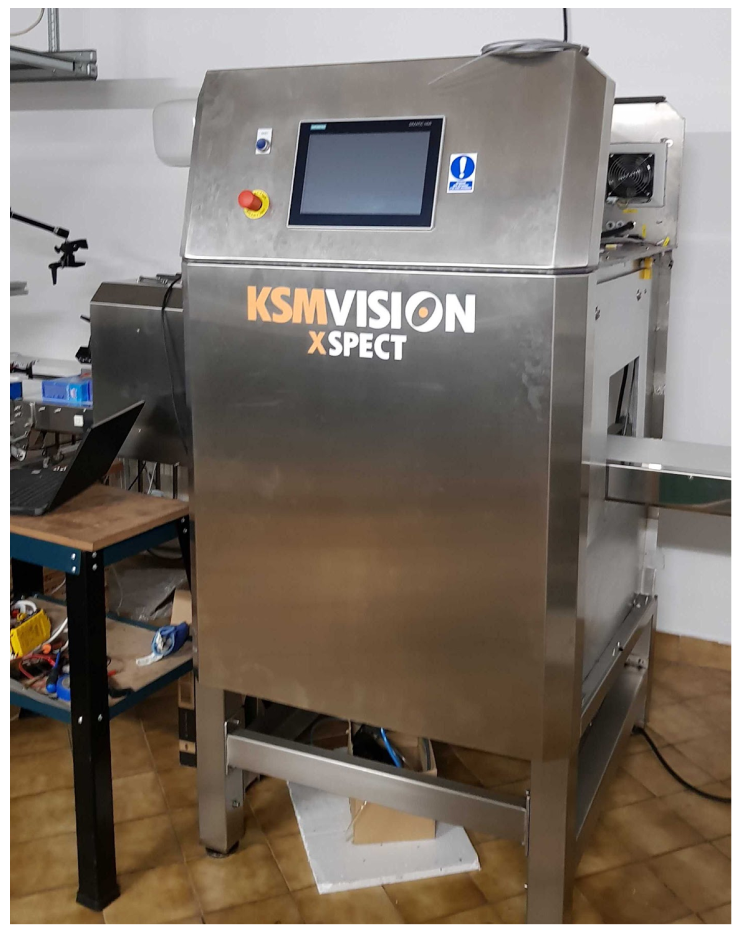
The developed anomaly detection system was used to search for foreign bodies in jars of pickled cucumbers. For this purpose, a device equipped with an X-ray source, a detector, a linear conveyor, and radiation protection covers was used (see Figure 6).
Figure 6. The KSM Vision Xspect device.
As part of the development of the foreign body detection system, several methods were used to compare them and select the best one. In each case, photos were taken of nondefective jars (Figure 7) and defective ones (Figure 8), i.e., those with various foreign bodies made of metal, rubber, and glass, and photos of these jars were taken. Some photos were used to train the models and the rest for testing. The size of the nondefective training set was 357 images, the defective testing set had 215, and the nondefective testing set had 200 images.
Figure 7. A normal jar (without any foreign body).
Figure 8. A defective jar (with several washers inside).
The same image preprocessing was used for all methods, i.e., jar localization by edge detection, limiting the data range by thresholding, gamma correction, and noise reduction.
The data prepared in this way were used for four methods: 1. Fine-tuning pretrained Xception, ResNet50, and InceptionV3 networks; 2. Developing own convolutional neural network; 3. Anomaly detection by background subtraction; 4. Using an autoencoder as an anomaly detector.
X-ray images are specific due to high noise rate and dynamic image depth range, so using fine-tuned pretrained models yielded results of only 68% in correct defect detecting. This is because these models were not trained on data resembling X-ray images. An artificial network designed by our own gave much better results (85% correct predictions), but in this case, the amount of training data was too small to achieve an even better result. A simple background subtraction algorithm was also used (the background was averaged over dozens of nondefective photos). This resulted in a high jar prediction efficiency of 95%. However, the high result of this method results from the use of features of a specific product, so it has little generalization, so it might not work on other products. Finally, the raw data were used to train the anomaly detector. The results in this case differ and depend on which part of the jar was examined. The middle part of the jar achieved 94% True Negative and 56% True Positive. The results are 90% True Positive, and 41% True Negative for the same part of the jar when the photos were divided into segments.
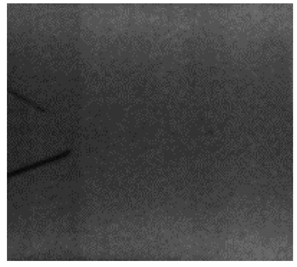
Another experiment used more complex preprocessing of X-ray images containing the same jars (the same dataset as described above was exercised). Images were binarized using adaptive thresholding, with a threshold value to retain all foreign bodies. This also resulted in some minor background noise remaining in the binary image, but this prevented information about the foreign bodies from being lost (see Figure 9 and Figure 10).
Figure 9. A cropped region of interest (ROI) with foreign body (a metal wire) seen on the left.
Figure 10. ROI from image Figure 9 preprocessed and resized.
Using this preprocessing, nondefect images (with jars containing no foreign bodies) were processed by the anomaly detector described in this paper. Firstly, images were used for feature detection by an extractor based on the OpenVino model (pretrained on the ImageNet dataset). These features were used to train an anomaly detector using an autoencoder. This algorithm was then tested on other sets of nondefective and defective jars. Although this method required a set of several faulty images to determine the threshold value, which is unusual for anomaly detectors, it still achieved good results. The minimum size of the training dataset for such an algorithm was also assessed. Table 4 shows the results of this comparison. For every set from 350 to 150 samples, the accuracy is greater than 90%. Only when the number of training samples is fewer than 150 does the algorithm classify all samples as good or bad. Applying an anomaly detector to a binary image made it possible to obtain an algorithm practically insensitive to very high noise, which is usually the case with X-ray images. The learning time achieved was 10 s for the set containing 357 samples.
Table 4. Accuracy of the algorithm depending on the size of the training set size. Values are percentages, so they point out how many samples were classified correctly (“good” and “faulty” for nondefective and defective sets, respectively). In this case, the accuracy of the training set was below 100%. Values are approximately repeatable for sets greater than 100.
For comparison, the results reported in [51] give an effectiveness of 91–94%. In this case, air bubbles are detected in the engine body. Researchers use a three-level autoencoder. The results are comparable, but the algorithm described requires a huge set of defective images for training, which may be challenging to meet in many applications. In [63], researchers trained the YOLOv4 model and achieved 94% efficiency when looking for foreign bodies in food in X-ray images. However, in the work in [64], which examined tire defects using X-ray, an autoencoder-based anomaly detector achieved an efficiency of at best 68%.
So far, the anomaly detector results require improvement, but some indicators are satisfactorily high. Work is still being carried out to improve the prediction efficiency of this anomaly detector in X-ray images. Since the anomaly detector only needs normal data, obtaining it is cheaper and more straightforward, which is essential in the case of a device such as an X-ray. Hence, there is a need to continue work and develop the anomaly detector model.

5. Conclusions and Future Works

In conclusion, this paper addresses the imperative need for stringent quality control in pharmaceutical and food manufacturing, encompassing both production and packaging processes. The utilization of machine vision technologies, coupled with deep neural network algorithms, has emerged as a pivotal standard, surpassing manual inspection methods. These technologies provide noncontact, consistent, and high-speed inspection capabilities.
However, challenges arise in contract manufacturing scenarios, where diverse formats necessitate frequent retraining of defect detection models. This recurrent format change, occurring multiple times a day, can lead to significant production downtime and system startup inefficiencies, especially in industries such as pharmaceutical blister packaging and bottle capping.
To surmount these challenges, we introduce an ultra-lightweight anomaly detector that is fast both in inference and training. This solution demonstrates its effectiveness in various quality control applications, including drugs in blisters, liquid packaging closures, and detecting foreign bodies in food packaging using X-ray imaging, as shown above.
In the future, we intend to train a feature extractor model from scratch on a large set of industrial data to increase the accuracy and ease of adaptation to production conditions. The current instantiation of the feature extractor employs training on the ImageNet dataset, facilitating the extraction of generalized features applicable to a broad spectrum of input images. However, the feature extraction can be enhanced by training the model on a dataset tailored to specific industrial domain. This will empower the model to generate features that are specifically attuned to the industrial data.
In summary, our proposed solution significantly advances the field, offering a versatile and efficient approach to quality control in diverse manufacturing settings. We anticipate that this work will pave the way for further innovations and enhancements in this critical domain.

Author Contributions

Conceptualization, M.K. and M.M.; Methodology, M.K.; Software, M.K.; Validation, J.R.; Writing—original draft, J.R.; Writing—review & editing, M.M. All authors have read and agreed to the published version of the manuscript.

Funding

This research was funded by the National Centre of Research and Development from European Union Funds under the Smart Growth Operational Programme, grants numbers: POIR.01.01.01-00-0097/17-00 and POIR.01.01.01-00-0488/20.

Institutional Review Board Statement

Not applicable.

Data Availability Statement

The source code and data used to support the findings of this study are available from the corresponding author upon request.

Acknowledgments

Authors greatly acknowledge the support from whole KSM Vision engineering Team, especially Piotr Rajkiewicz.

Conflicts of Interest

Authors Michał Kocon and Marcin Malesa were employed by the company KSM Vision sp. z o.o. The authors declare that the research was conducted in the absence of any commercial or financial relationships that could be construed as potential conflicts of interest.

References

  1. Montgomery, D.C. Introduction to Statistical Quality Control, 5th ed.; John Wiley: Hoboken, NJ, USA, 2005. [Google Scholar]
  2. Avigdor, Z.; Kenett, R.S. Quality 4.0—the challenging future of quality engineering. Qual. Eng. 2020, 32, 614–626. [Google Scholar]
  3. Villalba-Diez, J.; Schmidt, D.; Gevers, R.; Ordieres-Meré, J.; Buchwitz, M.; Wellbrock, W. Deep learning for industrial computer vision quality control in the printing industry 4.0. Sensors 2019, 19, 3987. [Google Scholar] [CrossRef] [PubMed]
  4. Nascimento, R.; Martins, I.; Dutra, T.A.; Moreira, L. Computer vision based quality control for additive manufacturing parts. Int. J. Adv. Manuf. Technol. 2023, 124, 3241–3256. [Google Scholar] [CrossRef]
  5. Longfei, Z.; Zhang, L.; Konz, N. Computer vision techniques in manufacturing. IEEE Trans. Syst. Man Cybern. Syst. 2022, 53, 105–117. [Google Scholar]
  6. Jinjiang, W.; Fu, P.; Gao, R.X. Machine vision intelligence for product defect inspection based on deep learning and Hough transform. J. Manuf. Syst. 2019, 51, 52–60. [Google Scholar]
  7. Luo, Q.; Fang, X.; Liu, L.; Yang, C.; Sun, Y. Automated visual defect detection for flat steel surface: A survey. IEEE Trans. Instrum. Meas. 2020, 69, 626–644. [Google Scholar] [CrossRef]
  8. Ciberlin, J.; Grbic, R.; Teslić, N.; Pilipović, M. Object detection and object tracking in front of the vehicle using front view camera. In Proceedings of the 2019 Zooming Innovation in Consumer Technologies Conference (ZINC), Novi Sad, Serbia, 29–30 May 2019. [Google Scholar]
  9. Monika, B.; Kumar, M.; Kumar, M. 2D object recognition: A comparative analysis of SIFT, SURF and ORB feature descriptors. Multimed. Tools Appl. 2021, 80, 18839–18857. [Google Scholar]
  10. Zhou, W.; Gao, S.; Zhang, L.; Lou, X. Histogram of oriented gradients feature extraction from raw bayer pattern images. IEEE Trans. Circuits Syst. II Express Briefs 2020, 67, 946–950. [Google Scholar] [CrossRef]
  11. Kumar, S.D.; Esakkirajan, S.; Bama, S.; Keerthiveena, B. A microcontroller based machine vision approach for tomato grading and sorting using SVM classifier. Microprocess. Microsyst. 2020, 76, 103090. [Google Scholar] [CrossRef]
  12. Abrar, A.; Jalal, A.; Kim, K. Region and decision tree-based segmentations for Multi-objects detection and classification in Outdoor Scenes. In Proceedings of the 2019 International Conference on Frontiers of Information Technology (FIT), Islamabad, Pakistan, 16–18 December 2019. [Google Scholar]
  13. Rachana, P.; Patel, S. A comprehensive study of applying convolutional neural network for computer vision. Int. J. Adv. Sci. Technol. 2020, 6, 2161–2174. [Google Scholar]
  14. Bhatt, D.; Patel, C.; Talsania, H.; Patel, J.; Vaghela, R.; Pandya, S.; Ghayvat, H. CNN variants for computer vision: History, architecture, application, challenges and future scope. Electronics 2021, 10, 2470. [Google Scholar] [CrossRef]
  15. Esteva, A.; Chou, K.; Yeung, S.; Naik, N.; Madani, A.; Mottaghi, A.; Liu, Y.; Topol, E.; Dean, J.; Socher, R. Deep learning-enabled medical computer vision. NPJ Digit. Med. 2021, 4, 5. [Google Scholar] [CrossRef]
  16. Magnus, E. Learning Deep Learning: Theory and Practice of Neural Networks, Computer Vision, Natural Language Processing, and Transformers Using TensorFlow; Addison-Wesley Professional: Boston, MA, USA, 2021. [Google Scholar]
  17. O’Mahony, N.; Campbell, S.; Carvalho, A.; Harapanahalli, S.; Hernandez, G.V.; Krpalkova, L.; Riordan, D.; Walsh, J. Deep learning vs. traditional computer vision. In Proceedings of the 2019 Computer Vision Conference (CVC), Las Vegas, NV, USA, 25–26 April 2019; Volume 1. [Google Scholar]
  18. Ahmed, M.; Anwar, A.; Mahmood, A.N.; Shah, Z.; Maher, M.J. An investigation of performance analysis of anomaly detection techniques for big data in scada systems. Eai Endorsed Trans. Ind. Netw. Intell. Syst. 2015, 2, e5. [Google Scholar] [CrossRef][Green Version]
  19. Pooja, K.; Sugandhi, R. Anomaly detection for predictive maintenance in industry 4.0—A survey. In Proceedings of the 6th International Conference on Energy and City of the Future (EVF’2019), Pune City, India, 18–20 December 2019; Volume 170. [Google Scholar][Green Version]
  20. Susto, G.A.; Terzi, M.; Beghi, A. Anomaly detection approaches for semiconductor manufacturing. Procedia Manuf. 2017, 11, 2018–2024. [Google Scholar] [CrossRef]
  21. Chandola, V.; Banerjee, A.; Kumar, V. Anomaly detection: A survey. ACM Comput. Surv. 2009, 41, 1–58. [Google Scholar] [CrossRef]
  22. Bhuyan, M.H.; Bhattacharyya, D.K.; Kalita, J.K. Network anomaly detection: Methods, systems and tools. IEEE Commun. Surv. Tutor. 2013, 16, 303–336. [Google Scholar] [CrossRef]
  23. Choi, K.; Yi, J.; Park, C.; Yoon, S. Deep Learning for Anomaly Detection in Time-Series Data: Review, Analysis, and Guidelines. IEEE Access 2021, 9, 120043–120065. [Google Scholar] [CrossRef]
  24. Roth, K.; Pemula, L.; Zepeda, J.; Schölkopf, B.; Brox, T.; Gehler, P. Towards Total Recall in Industrial Anomaly Detection. In Proceedings of the IEEE/CVF Conference on Computer Vision and Pattern Recognition, New Orleans, LA, USA, 18–24 June 2022. [Google Scholar]
  25. Ding, K.; Zhang, J.; Ding, H.; Liu, Y.; Chen, F.; Li, Y. Fault detection of photovoltaic array based on Grubbs criterion and local outlier factor. Iet Renew. Power Gener. 2020, 14, 551–559. [Google Scholar] [CrossRef]
  26. Gu, X.; Akoglu, L.; Rinaldo, A. Statistical analysis of nearest neighbor methods for anomaly detection. In Proceedings of the 2019 Conference on Neural Information Processing Systems, Vancouver, BC, Canada, 8–14 December 2019; Volume 32. [Google Scholar]
  27. Leon-Lopez, K.M.; Mouret, F.; Arguello, H.; Tourneret, J.Y. Anomaly detection and classification in multispectral time series based on hidden Markov models. IEEE Trans. Geosci. Remote. Sens. 2021, 60, 1–11. [Google Scholar] [CrossRef]
  28. Gong, D.; Liu, L.; Le, V.; Saha, B.; Mansour, M.R.; Venkatesh, S.; Hengel, A.V.D. Memorizing normality to detect anomaly: Memory-augmented deep autoencoder for unsupervised anomaly detection. In Proceedings of the IEEE/CVF International Conference on Computer Vision, Seoul, Republic of Korea, 27 October–2 November 2019. [Google Scholar]
  29. Ahmad, Z.; Shahid Khan, A.; Nisar, K.; Haider, I.; Hassan, R.; Haque, M.R.; Tarmizi, S.; Rodrigues, J.J.P.C. Anomaly detection using deep neural network for IoT architecture. Appl. Sci. 2021, 11, 7050. [Google Scholar] [CrossRef]
  30. Omar, S.; Ngadi, A.; Jebur, H.H. Machine Learning Techniques for Anomaly Detection: An Overview. Int. J. Comput. Appl. 2013, 79, 33–41. [Google Scholar] [CrossRef]
  31. Zhou, Y.; Song, X.; Zhang, Y.; Liu, F.; Zhu, C.; Liu, L. Feature encoding with autoencoders for weakly supervised anomaly detection. IEEE Trans. Neural Netw. Learn. Syst. 2021, 33, 2454–2465. [Google Scholar] [CrossRef] [PubMed]
  32. Shujian, Y.; Príncipe, J.C. Understanding Autoencoders with Information Theoretic Concepts. Neural Netw. 2019, 117, 104–123. [Google Scholar]
  33. Qian, J.; Song, Z.; Yao, Y.; Zhu, Z.; Zhang, X. A Review on Autoencoder Based Representation Learning for Fault Detection and Diagnosis in Industrial Processes. Chemom. Intell. Lab. Syst. 2022, 231, 104711. [Google Scholar] [CrossRef]
  34. Charte, D.; Charte, F.; del Jesus, M.J.; Herrera, F. An analysis on the use of autoencoders for representation learning: Fundamentals, learning task case studies, explainability and challenges. Neurocomputing 2020, 404, 93–107. [Google Scholar] [CrossRef]
  35. Song, Y.; Hyun, S.; Cheong, Y.G. Analysis of autoencoders for network intrusion detection. Sensors 2021, 21, 4294. [Google Scholar] [CrossRef] [PubMed]
  36. Nguyen, D.T.; Lou, Z.; Klar, M.; Brox, T. Anomaly Detection With Multiple-Hypotheses Predictions. Int. Conf. Mach. Learn. 2019, 4800–4809. [Google Scholar]
  37. Liu, J.; Song, K.; Feng, M.; Yan, Y.; Tu, Z.; Zhu, L. Semi-supervised Anomaly Detection with Dual Prototypes Autoencoder for Industrial Surface Inspection. Opt. Lasers Eng. 2021, 136, 106324. [Google Scholar] [CrossRef]
  38. Angelov, S.; Lazarova, M. Convolutional Autoencoders for Image Comparison in Printing Industry Quality Control. In Proceedings of the 2022 10th International Scientific Conference on Computer Science (COMSCI), Sofia, Bulgaria, 30 May–2 June 2022. [Google Scholar]
  39. Kozamernik, N.; Bračun, D. Visual inspection system for anomaly detection on KTL coatings using variational autoencoders. Procedia CIRP 2020, 93, 1558–1563. [Google Scholar] [CrossRef]
  40. Heger, J.; Desai, G.; El Abdine, M.Z. Anomaly detection in formed sheet metals using convolutional autoencoders. Procedia CIRP 2020, 93, 1281–1285. [Google Scholar] [CrossRef]
  41. Niu, T.; Li, B.; Li, W.; Qiu, Y.; Niu, S. Positive-sample-based surface defect detection using memory-augmented adversarial autoencoders. IEEE ASME Trans. Mechatron. 2021, 27, 46–57. [Google Scholar] [CrossRef]
  42. Kim, J.; Ko, J.; Choi, H.; Kim, H. Printed circuit board defect detection using deep learning via a skip-connected convolutional autoencoder. Sensors 2021, 21, 4968. [Google Scholar] [CrossRef] [PubMed]
  43. Maggipinto, M.; Beghi, A.; Susto, G.A. A deep convolutional autoencoder-based approach for anomaly detection with industrial, non-images, 2-dimensional data: A semiconductor manufacturing case study. IEEE Trans. Autom. Sci. Eng. 2022, 19, 1477–1490. [Google Scholar] [CrossRef]
  44. Ren, H.; Chai, Y.; Qu, J.; Zhang, K.; Tang, Q. An intelligent fault detection method based on sparse auto-encoder for industrial process systems: A case study on tennessee eastman process chemical system. In Proceedings of the 2018 10th International Conference on Intelligent Human-Machine Systems and Cybernetics (IHMSC), Hangzhou, China, 25–26 August 2018; Volume 1. [Google Scholar]
  45. Zhu, J.; Jiang, M.; Liu, Z. Fault detection and diagnosis in industrial processes with variational autoencoder: A comprehensive study. Sensors 2021, 22, 227. [Google Scholar] [CrossRef] [PubMed]
  46. Davletshina, D.; Melnychuk, V.; Tran, V.; Singla, H.; Berrendorf, M.; Faerman, E.; Fromm, M.; Schubert, M. Unsupervised Anomaly Detection for X-Ray Images. arXiv 2020, arXiv:2001.10883. [Google Scholar]
  47. Mao, Y.; Xue, F.F.; Wang, R.; Zhang, J.; Zheng, W.S.; Liu, H. Abnormality detection in chest X-ray images using uncertainty prediction autoencoders. In Proceedings of the Medical Image Computing and Computer Assisted Intervention–MICCAI 2020: 23rd International Conference, Proceedings, Part VI 23, Lima, Peru, 4–8 October 2020; Springer: Berlin/Heidelberg, Germany, 2020. [Google Scholar]
  48. Tekawade, A.; Liu, Z.; Kenesei, P.; Bicer, T.; De Carlo, F.; Kettimuthu, R.; Foster, I. 3d autoencoders for feature extraction in X-ray tomography. In Proceedings of the 2021 IEEE International Conference on Image Processing (ICIP), Anchorage, AK, USA, 19–22 September 2021. [Google Scholar]
  49. Presenti, A.; Liang, Z.; Alves Pereira, L.F.; Sijbers, J.; De Beenhouwer, J. Automatic anomaly detection from X-ray images based on autoencoders. Nondestruct. Test. Eval. 2022, 37, 552–565. [Google Scholar] [CrossRef]
  50. Tang, W.; Vian, C.M.; Tang, Z.; Yang, B. Anomaly detection of core failures in die casting X-ray inspection images using a convolutional autoencoder. Mach. Vis. Appl. 2021, 32, 102. [Google Scholar] [CrossRef]
  51. Ren, J.; Ren, R.; Green, M.; Huang, X. Defect detection from X-ray images using a three-stage deep learning algorithm. In Proceedings of the 2019 IEEE Canadian Conference of Electrical and Computer Engineering (CCECE), Edmonton, AB, Canada, 5–8 May 2019. [Google Scholar]
  52. Sandler, M.; Howard, A.; Zhu, M.; Zhmoginov, A.; Chen, L.C. MobileNetV2: Inverted Residuals and Linear Bottlenecks. In Proceedings of the 2018 IEEE/CVF Conference on Computer Vision and Pattern Recognition, Salt Lake City, UT, USA, 18–23 June 2018; pp. 4510–4520. [Google Scholar]
  53. Deng, J.; Dong, W.; Socher, R.; Li, L.J.; Li, K.; Fei-Fei, L. ImageNet: A large-scale hierarchical image database. In Proceedings of the 2009 IEEE Conference on Computer Vision and Pattern Recognition, Miami, FL, USA, 20–25 June 2009; pp. 248–255. [Google Scholar]
  54. Bergmann, P.; Batzner, K.; Fauser, M.; Sattlegger, D.; Steger, C. The MVTec Anomaly Detection Dataset: A Comprehensive Real-World Dataset for Unsupervised Anomaly Detection. Int. J. Comput. Vis. 2021, 129, 1038–1059. [Google Scholar] [CrossRef]
  55. Bergmann, P.; Fauser, M.; Sattlegger, D.; Steger, C. MVTec AD—A Comprehensive Real-World Dataset for Unsupervised Anomaly Detection. In Proceedings of the IEEE/CVF Conference on Computer Vision and Pattern Recognition (CVPR), Long Beach, CA, USA, 15–20 June 2019; pp. 9584–9592. [Google Scholar]
  56. Malesa, M.; Rajkiewicz, P. Quality Control of PET Bottles Caps with Dedicated Image Calibration and Deep Neural Networks. Sensors 2021, 21, 501. [Google Scholar] [CrossRef]
  57. Yu, J.; Zheng, Y.; Wang, X.; Li, W.; Wu, Y.; Zhao, R.; Wu, L. FastFlow: Unsupervised Anomaly Detection and Localization via 2D Normalizing Flows. arXiv 2021, arXiv:2111.07677. [Google Scholar]
  58. Batzner, K.; Heckler, L.; König, R. EfficientAD: Accurate Visual Anomaly Detection at Millisecond-Level Latencies. arXiv 2023, arXiv:2303.14535. [Google Scholar]
  59. Ahuja, N.A.; Ndiour, I.; Kalyanpur, T.; Tickoo, O. Probabilistic Modeling of Deep Features for Out-of-Distribution and Adversarial Detection. arXiv 2019, arXiv:1909.11786. [Google Scholar]
  60. Defard, T.; Setkov, A.; Loesch, A.; Audigier, R. PaDiM: A Patch Distribution Modeling Framework for Anomaly Detection and Localization. In International Conference on Pattern Recognition; Springer International Publishing: Cham, Switzerland, 2021. [Google Scholar]
  61. Akcay, S.; Ameln, D.; Vaidya, A.; Lakshmanan, B.; Ahuja, N.; Genc, U. Anomalib: A Deep Learning Library for Anomaly Detection. In Proceedings of the 2022 IEEE International Conference on Image Processing (ICIP), Bordeaux, France, 16–19 October 2022; pp. 1706–1710. [Google Scholar]
  62. Intel® Distribution of OpenVINO™ Toolkit. Available online: https://www.intel.com/content/www/us/en/developer/tools/openvino-toolkit/overview.html (accessed on 1 December 2023).
  63. Kim, K.; Kim, H.; Chun, J.; Kang, M.; Hong, M.; Min, B. Real-Time Anomaly Detection in Packaged Food X-Ray Images Using Supervised Learning. Comput. Mater. Contin. 2021, 67, 2547–2568. [Google Scholar] [CrossRef]
  64. Wang, Y.; Zhang, Y.; Zheng, L.; Yin, L.; Chen, J.; Lu, J. Unsupervised Learning with Generative Adversarial Network for Automatic Tire Defect Detection from X-ray Images. Sensors 2021, 21, 6773. [Google Scholar] [CrossRef]
Disclaimer/Publisher’s Note: The statements, opinions and data contained in all publications are solely those of the individual author(s) and contributor(s) and not of MDPI and/or the editor(s). MDPI and/or the editor(s) disclaim responsibility for any injury to people or property resulting from any ideas, methods, instructions or products referred to in the content.

Article Metrics

Citations

Article Access Statistics

Multiple requests from the same IP address are counted as one view.