
A Machine Learning Approach to Robot Localization Using Fiducial Markers in RobotAtFactory 4.0 Competition

 ,
,  , ,
, ,  ,
,  ,
,  ,
,  ,
,  and
and 
Abstract
1. Introduction
2. State of the Art
3. Project Description
3.1. Theoretical Background
- Random Forest (RF) is an ensemble learning method that consists of a random combination of multiple decision trees. This method is a common approach to classification problems but can be used for regression as well [28].
- K-Nearest Neighbor Regression (KNR) is a regression version of the K-Nearest Neighbor (KNN) algorithm. This is one of the simplest and best-known non-parametric methods [29]. The main idea is to predict the target according to a local interpolation of the targets of the nearest neighbors in the training set (https://scikit-learn.org/stable/modules/generated/sklearn.neighbors.KNeighborsRegressor.html, accessed on 7 December 2022).
- Multilayer Perceptron (MLP) is a fully connected Artificial Neural Network (ANN) and was presented by [30]. It is composed of artificial neurons, whose model was proposed by [31]. MLP consists of at least three main layers: an input layer, a hidden layer (one or more), and an output layer. MLP uses the back-propagation learning technique for training [32].
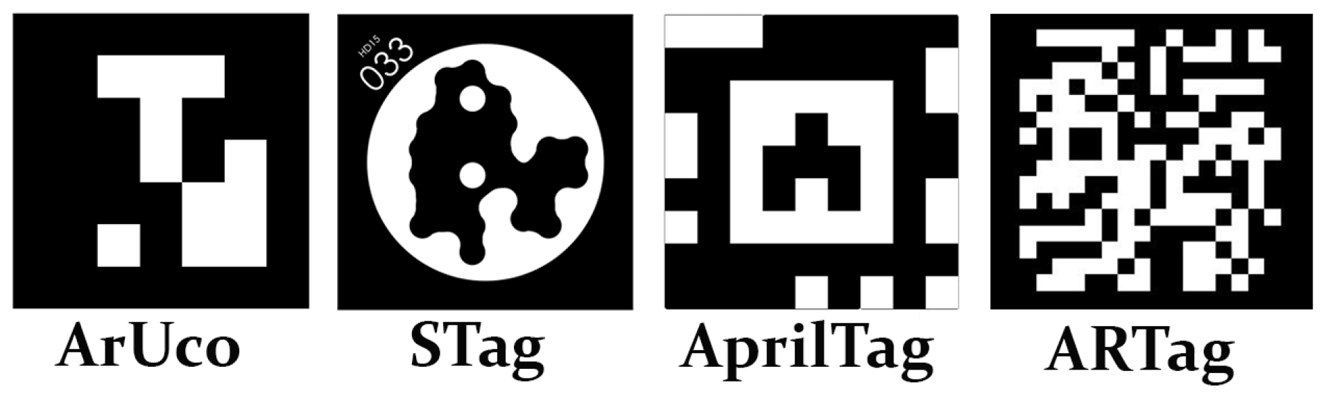
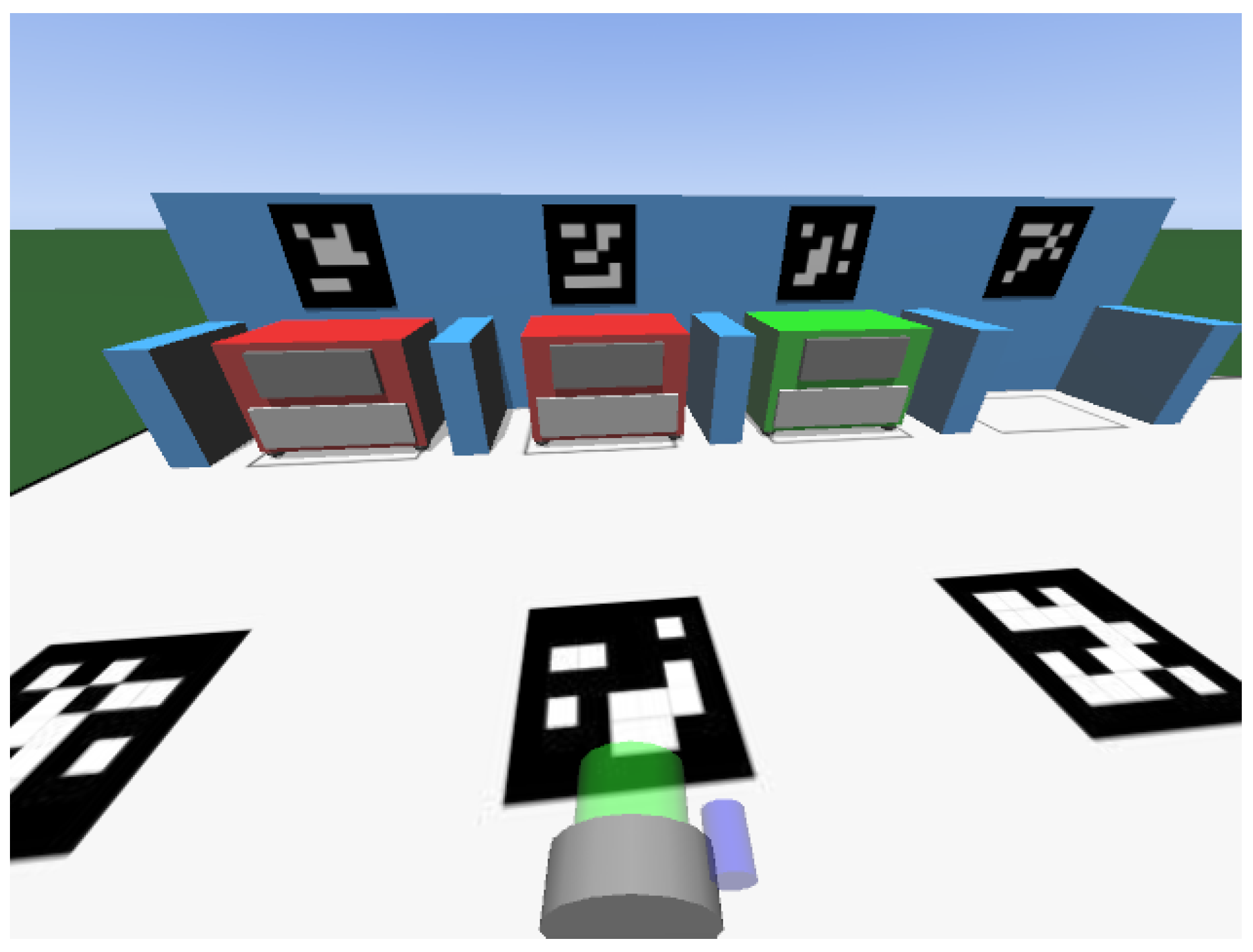
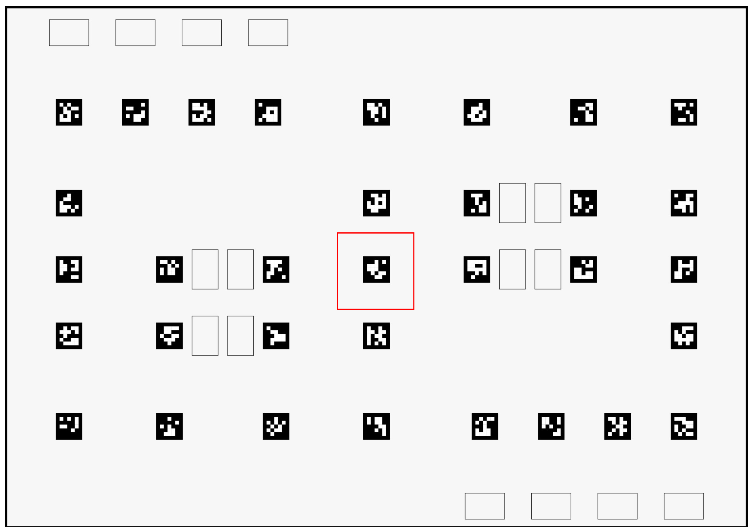
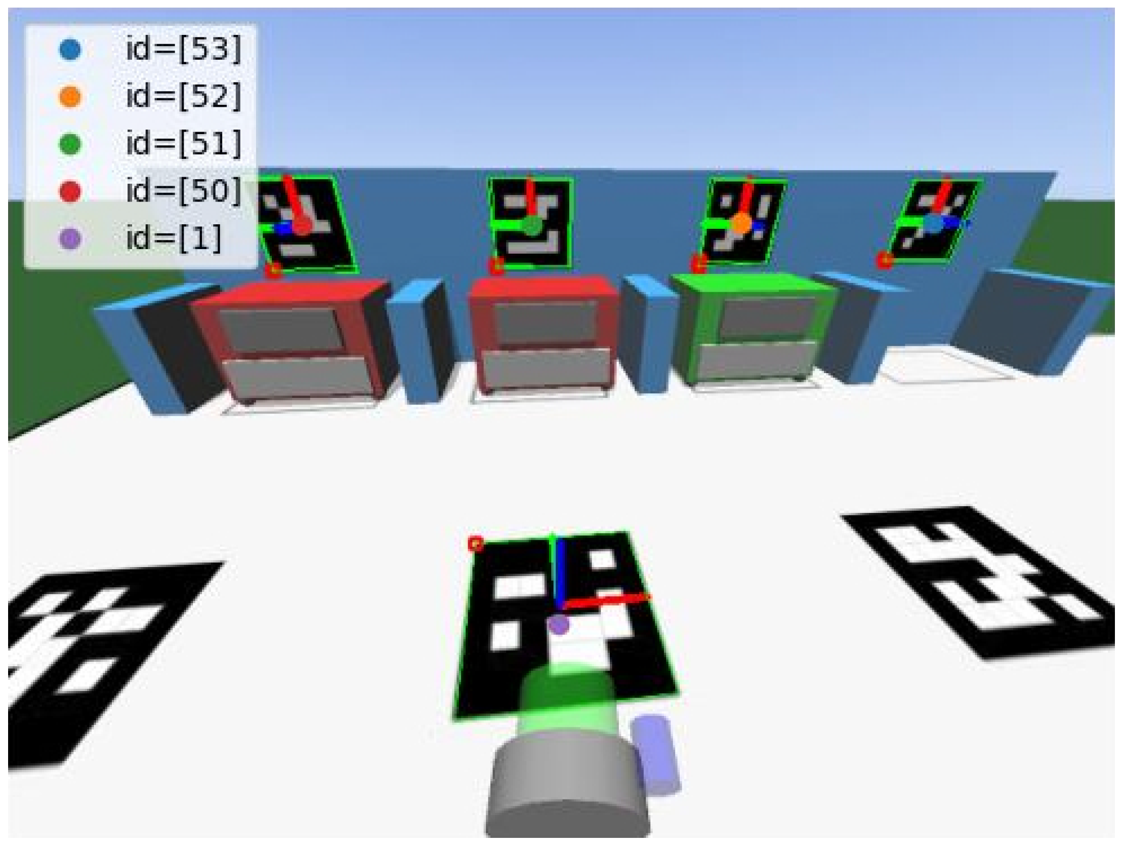
3.2. Fiducial Markers
3.3. Scenario Context
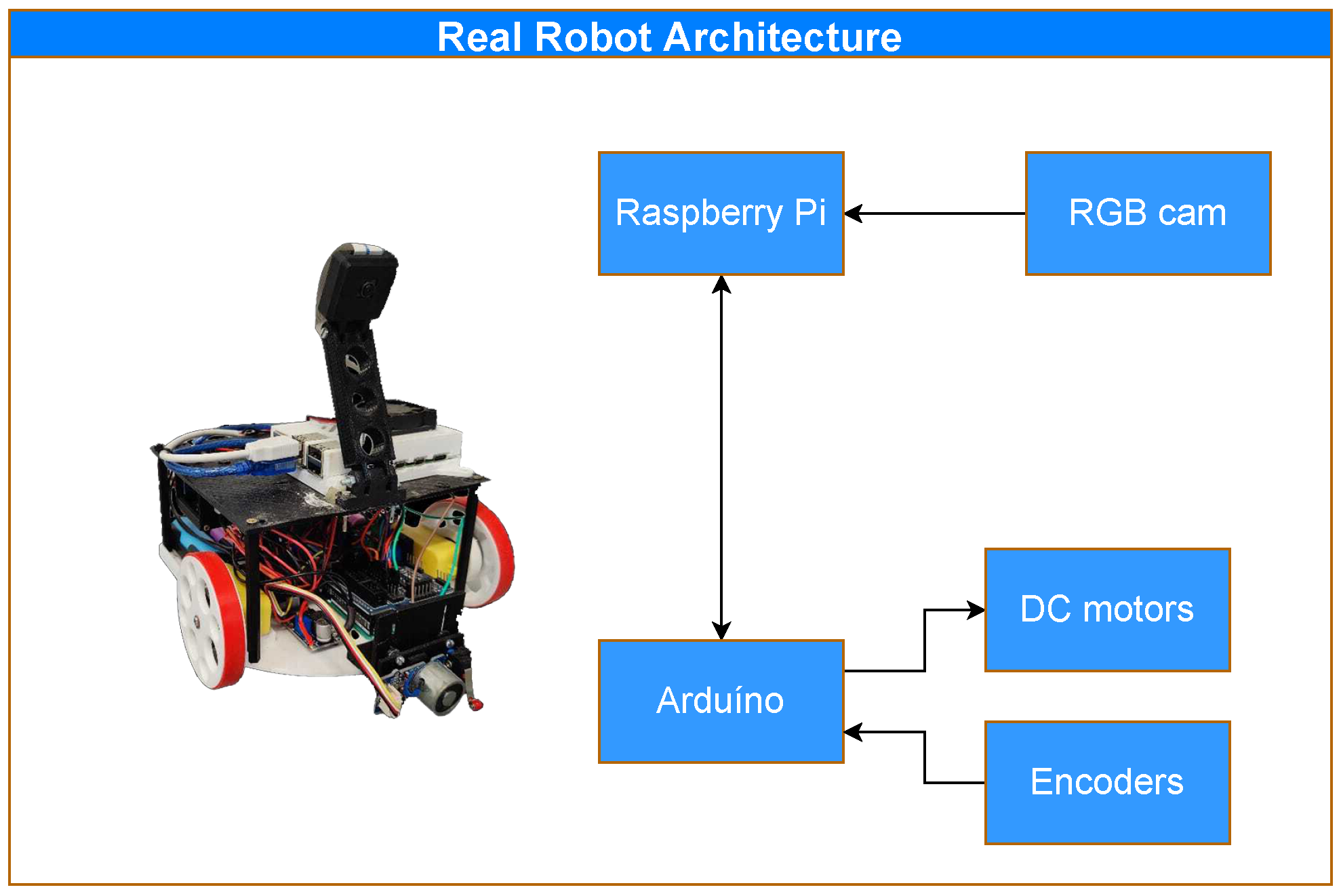
3.3.1. Robot
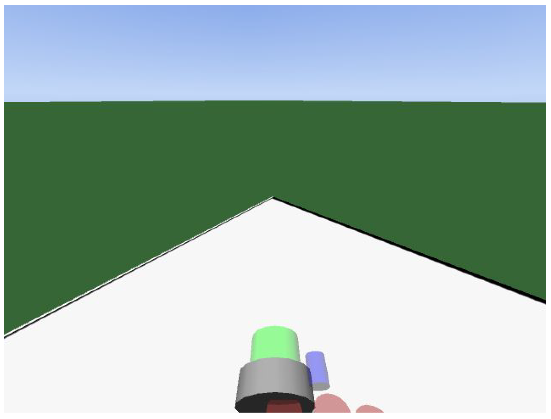
3.3.2. Realistic Simulator
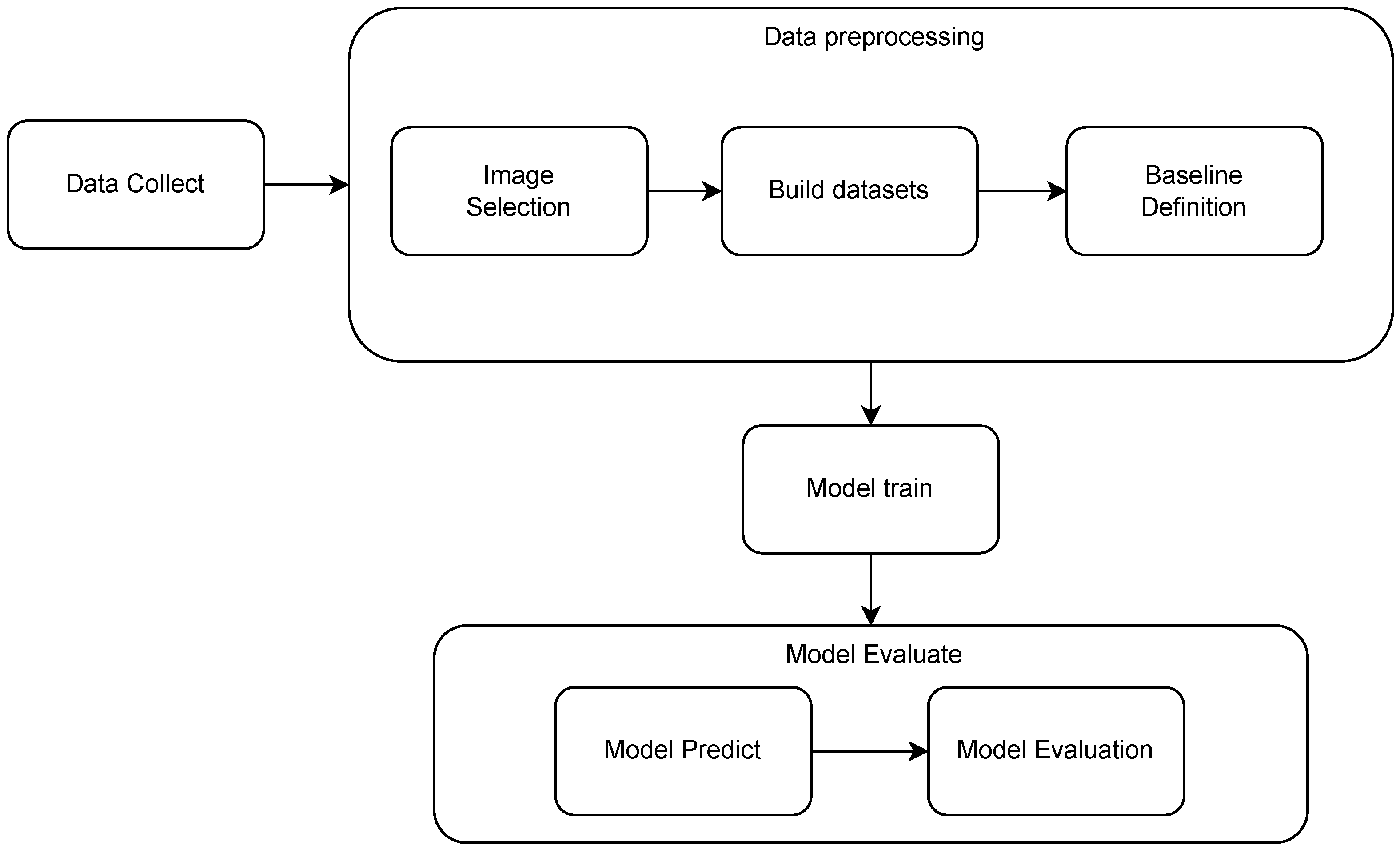
3.4. Methodology
3.4.1. Data Collection
3.4.2. Data Preprocessing
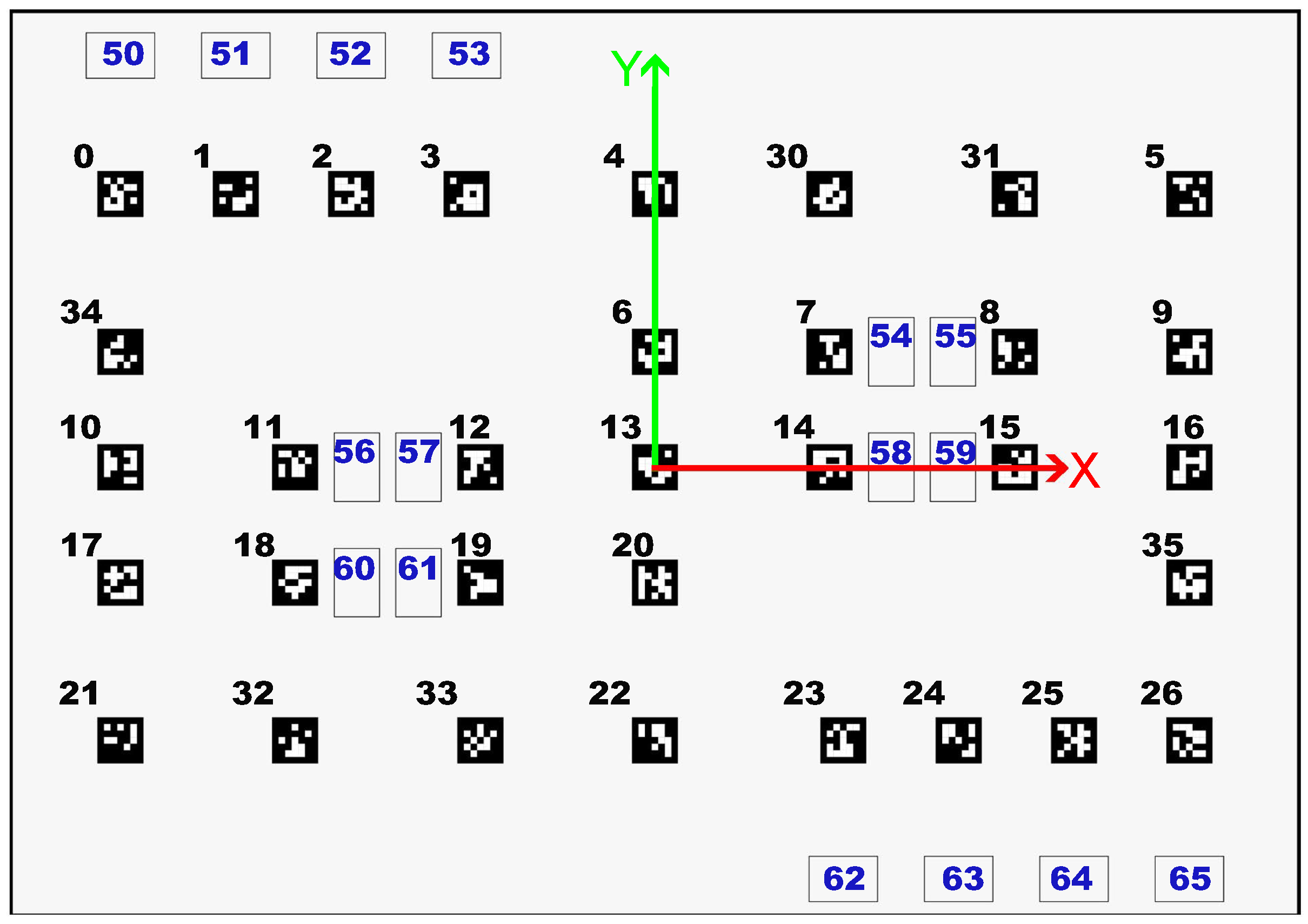
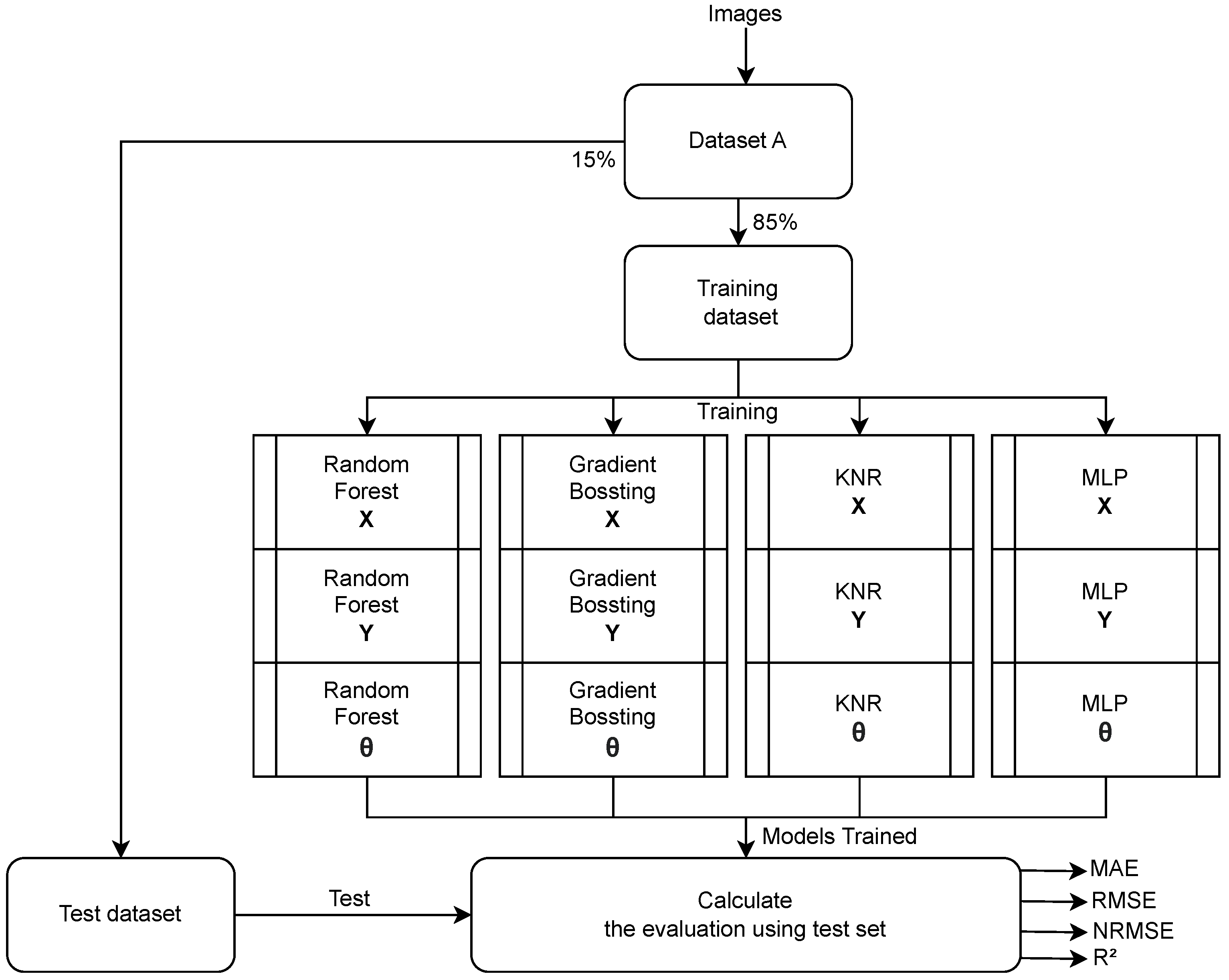
- Dataset A—Using images from the whole field and combining the observations’ attributes in a matrix format: The images used in this dataset were collected in the whole field considering a grid with a 1 cm resolution. In this, each observation in the dataset represents one image and has only one feature and 3 targets. The feature is a matrix with 49 lines (where each represents one ArUco) and 7 columns (where each represents the tvec and rvec array data and the last column serves to identify whether the marker was detected or not). In the cases in which an image does not contain a specific ArUco, the corresponding line in the matrix will be 0 (indicating the absence of the ArUco in that image). The target variables are x, y and .
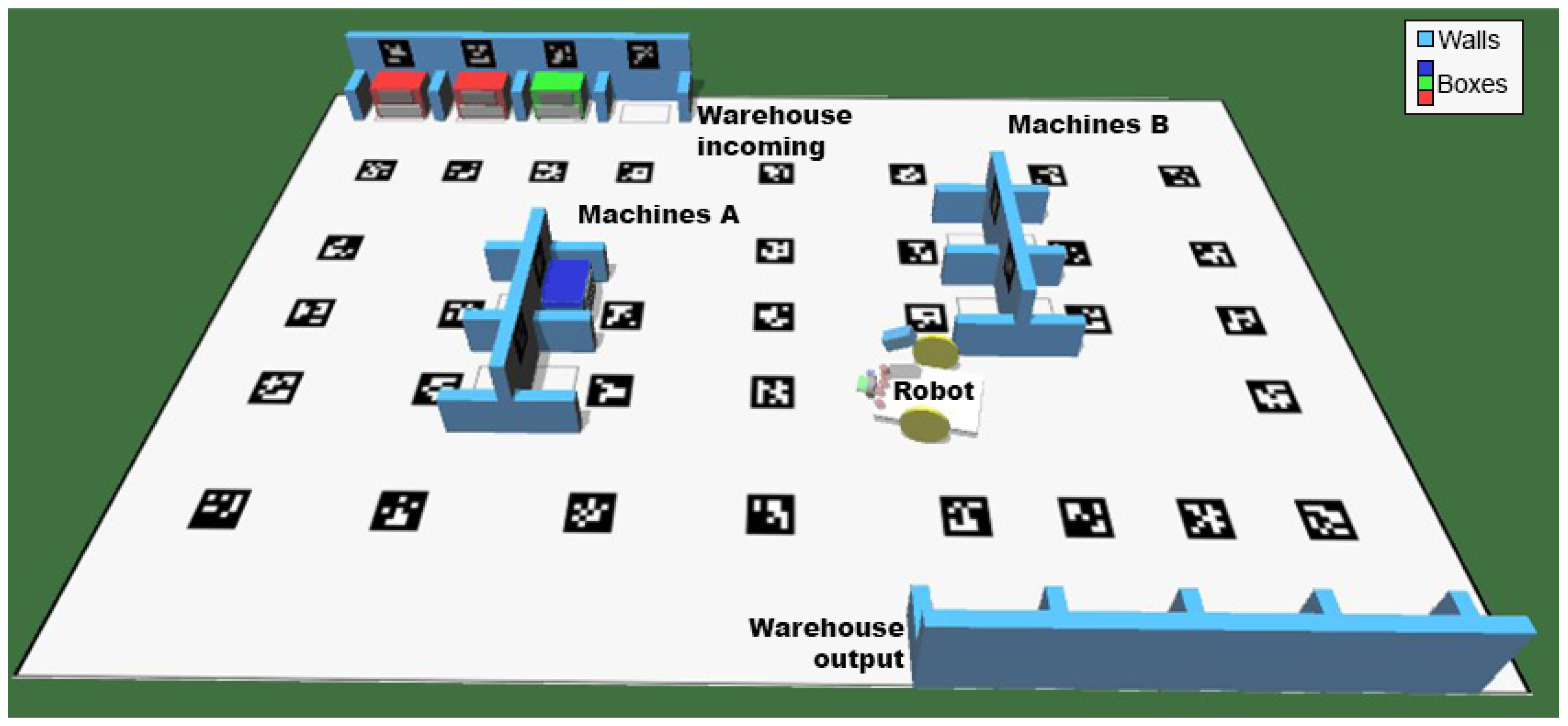
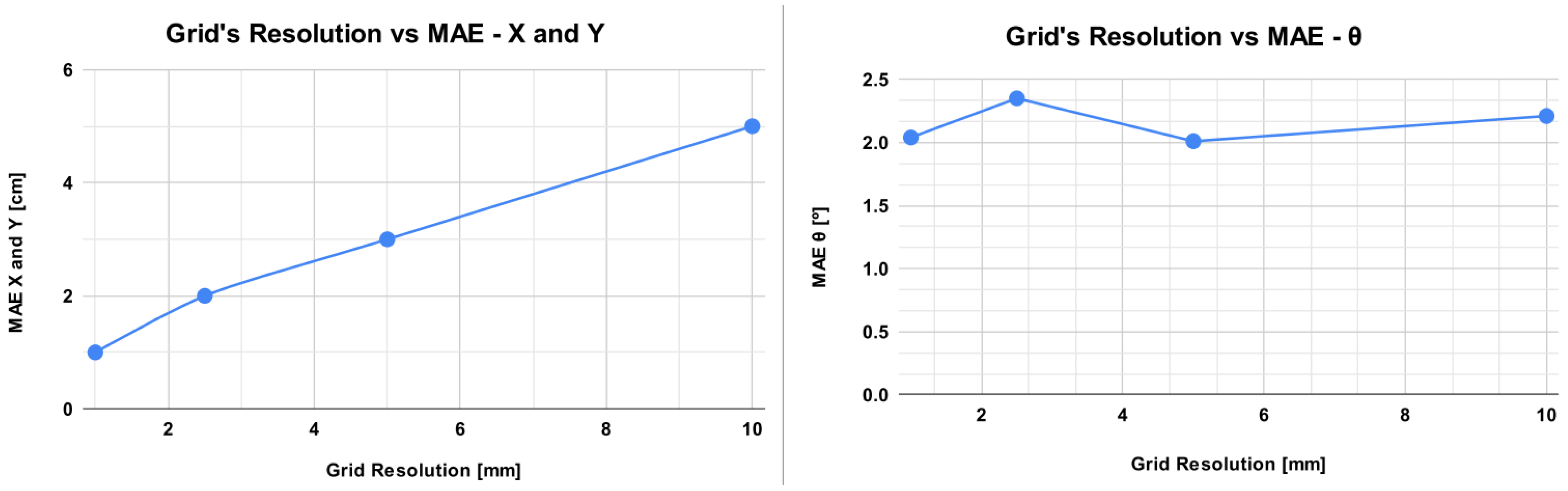
- Datasets B—Using images from the limited part of the field with different grid resolutions and combining the observations’ attributes in a matrix format: The images used in these datasets were collected in the center of the field (Figure 7) considering different grid resolutions. Four resolutions were used and four datasets were created: B1 with 10 mm, B2 with 5 mm, B3 with 2.5 mm, and B4 with 1 mm. The method to create each dataset was the same as presented for Dataset A.
- Dataset C—Using images from the whole field in an ArUco’s array: The images used in this dataset were collected in the whole field considering a grid with a 1 cm resolution. Instead of each observation representing an image, now, each one represents one detected ArUco. Thus, each observation is composed of seven features: the tag’s id, rvecs and tvecs; and three targets, x, y and . Thus, in this dataset, the information about the image is not relevant anymore, since the focus is on the relative pose of the ArUcos.
- Dataset D—Using images from a random route in an ArUco’s array: The images used in this dataset were collected in the whole field considering a random path. The method to create the dataset was the same as presented for Dataset C.
3.4.3. Processing and Model Definition
3.4.4. Model Evaluation
4. Results and Discussion
5. Conclusions
Author Contributions
Funding
Informed Consent Statement
Data Availability Statement
Acknowledgments
Conflicts of Interest
References
- Huang, S.; Dissanayake, G. Robot Localization: An Introduction. In Wiley Encyclopedia of Electrical and Electronics Engineering; John Wiley & Sons, Ltd.: Hoboken, NJ, USA, 2016; pp. 1–10. [Google Scholar] [CrossRef]
- Grewal, M.S.; Weill, L.R.; Andrews, A.P. Global Positioning Systems, Inertial Navigation, and Integration; John Wiley & Sons, Ltd.: Hoboken, NJ, USA, 2007. [Google Scholar]
- Nessa, A.; Adhikari, B.; Hussain, F.; Fernando, X.N. A Survey of Machine Learning for Indoor Positioning. IEEE Access 2020, 8, 214945–214965. [Google Scholar] [CrossRef]
- Braun, J.; Oliveira Júnior, A.; Berger, G.; Pinto, V.; Soares, I.; Pereira, A.; Lima, J.; Costa, P. A robot localization proposal for the RobotAtFactory 4.0: A novel robotics competition within the Industry 4.0 concept. Front. Robot. AI 2022, 9, 1023590. [Google Scholar] [CrossRef] [PubMed]
- Kalman, R.E. A New Approach to Linear Filtering and Prediction Problems. J. Basic Eng. 1960, 82, 35–45. [Google Scholar] [CrossRef]
- Welch, G.; Bishop, G. An Introduction to the Kalman Filter; Technical Report; University of North Carolina at Chapel Hill: Chapel Hill, NC, USA, 2004. [Google Scholar]
- Russell, S.; Norvig, P. Artificial Intelligence: A Modern Approach, 3rd ed.; Prentice Hall: Hoboken, NJ, USA, 2010. [Google Scholar]
- Maybeck, P.S. The Kalman filter: An introduction to concepts. In Autonomous Robot Vehicles; Springer: Berlin/Heidelberg, Germany, 1990; pp. 194–204. [Google Scholar]
- Fox, D.; Burgard, W.; Thrun, S. Markov localization for mobile robots in dynamic environments. J. Artif. Intell. Res. 1999, 11, 391–427. [Google Scholar] [CrossRef]
- Gordon, N.J.; Salmond, D.J.; Smith, A.F. Novel approach to nonlinear/non-Gaussian Bayesian state estimation. IEE Proc. F Radar Signal Process 1993, 140, 107–113. [Google Scholar] [CrossRef]
- Arulampalam, M.S.; Maskell, S.; Gordon, N.; Clapp, T. A tutorial on particle filters for online nonlinear/non-Gaussian Bayesian tracking. IEEE Trans. Signal Process. 2002, 50, 174–188. [Google Scholar] [CrossRef]
- Fox, D.; Burgard, W.; Dellaert, F.; Thrun, S. Monte carlo localization: Efficient position estimation for mobile robots. AAAI/IAAI 1999, 1999, 2. [Google Scholar]
- Dellaert, F.; Fox, D.; Burgard, W.; Thrun, S. Monte Carlo localization for mobile robots. In Proceedings of the 1999 IEEE International Conference on Robotics and Automation (Cat. No.99CH36288C), Detroit, MI, USA, 10–15 May 1999; Volume 2, pp. 1322–1328. [Google Scholar] [CrossRef]
- Lauer, M.; Lange, S.; Riedmiller, M. Calculating the Perfect Match: An Efficient and Accurate Approach for Robot Self-localization. In RoboCup 2005: Robot Soccer World Cup IX; Bredenfeld, A., Jacoff, A., Noda, I., Takahashi, Y., Eds.; Springer: Berlin/Heidelberg, Gremany, 2006; pp. 142–153. [Google Scholar]
- Besl, P.; McKay, N.D. A method for registration of 3-D shapes. IEEE Trans. Pattern Anal. Mach. Intell. 1992, 14, 239–256. [Google Scholar] [CrossRef]
- Sobreira, H.; Costa, C.; Sousa, I.; Rocha, L.; Lima, J.; Farias, P.; Costa, P.; Moreira, A. Map-Matching Algorithms for Robot Self-Localization: A Comparison Between Perfect Match, Iterative Closest Point and Normal Distributions Transform. J. Intell. Robot. Syst. 2019, 93, 533–546. [Google Scholar] [CrossRef]
- Biber, P.; Strasser, W. The normal distributions transform: A new approach to laser scan matching. In Proceedings of the 2003 IEEE/RSJ International Conference on Intelligent Robots and Systems (IROS 2003) (Cat. No.03CH37453), Las Vegas, NV, USA, 27–31 October 2003; Volume 3, pp. 2743–2748. [Google Scholar] [CrossRef]
- Magnusson, M.; Nuchter, A.; Lorken, C.; Lilienthal, A.J.; Hertzberg, J. Evaluation of 3D registration reliability and speed—A comparison of ICP and NDT. In Proceedings of the 2009 IEEE International Conference on Robotics and Automation, Kobe, Japan, 12–17 May 2009; pp. 3907–3912. [Google Scholar] [CrossRef]
- Magnusson, M. The Three-Dimensional Normal-Distributions Transform: An Efficient Representation for Registration, Surface Analysis, and Loop Detection. Ph.D. Thesis, Örebro Universitet, Örebro, Sweden, 2009. [Google Scholar]
- Pullano, S.A.; Bianco, M.G.; Critello, D.C.; Menniti, M.; La Gatta, A.; Fiorillo, A.S. A Recursive Algorithm for Indoor Positioning Using Pulse-Echo Ultrasonic Signals. Sensors 2020, 20, 5042. [Google Scholar] [CrossRef]
- Kalaitzakis, M.; Cain, B.; Carroll, S.; Ambrosi, A.; Whitehead, C.; Vitzilaios, N. Fiducial markers for pose estimation. J. Intell. Robot. Syst. 2021, 101, 1–26. [Google Scholar] [CrossRef]
- de Oliveira Júnior, A.; Piardi, L.; Bertogna, E.G.; Leitão, P. Improving the Mobile Robots Indoor Localization System by Combining SLAM with Fiducial Markers. In Proceedings of the 2021 Latin American Robotics Symposium (LARS), 2021 Brazilian Symposium on Robotics (SBR), and 2021 Workshop on Robotics in Education (WRE), Natal, Brazil, 11–15 October 2021; pp. 234–239. [Google Scholar] [CrossRef]
- Sadeghi Esfahlani, S.; Sanaei, A.; Ghorabian, M.; Shirvani, H. The Deep Convolutional Neural Network Role in the Autonomous Navigation of Mobile Robots (SROBO). Remote Sens. 2022, 14, 3324. [Google Scholar] [CrossRef]
- Atanasyan, A.; Roßmann, J. Improving Self-Localization Using CNN-based Monocular Landmark Detection and Distance Estimation in Virtual Testbeds. In Tagungsband des 4. Kongresses Montage Handhabung Industrieroboter; Schüppstuhl, T., Tracht, K., Roßmann, J., Eds.; Springer: Berlin/Heidelberg, Germany, 2019; pp. 249–258. [Google Scholar]
- Kendall, A.; Grimes, M.; Cipolla, R. PoseNet: A Convolutional Network for Real-Time 6-DOF Camera Relocalization. In Proceedings of the 2015 IEEE International Conference on Computer Vision (ICCV), Santiago, Chile, 7–13 December 2015; pp. 2938–2946. [Google Scholar] [CrossRef]
- Szegedy, C.; Liu, W.; Jia, Y.; Sermanet, P.; Reed, S.; Anguelov, D.; Erhan, D.; Vanhoucke, V.; Rabinovich, A. Going deeper with convolutions. In Proceedings of the 2015 IEEE Conference on Computer Vision and Pattern Recognition (CVPR), Boston, MA, USA, 8–10 June 2015; pp. 1–9. [Google Scholar] [CrossRef]
- Kim, G.; Petriu, E.M. Fiducial marker indoor localization with Artificial Neural Network. In Proceedings of the 2010 IEEE/ASME International Conference on Advanced Intelligent Mechatronics, Montreal, QC, Canada, 6–9 July 2010; pp. 961–966. [Google Scholar] [CrossRef]
- Breiman, L. Random forests. Mach. Learn. 2001, 45, 5–32. [Google Scholar] [CrossRef]
- James, G.; Witten, D.; Hastie, T.; Tibshirani, R. An Introduction to Statistical Learning: With Applications in R; Springer: Berlin/Heidelberg, Germany, 2014. [Google Scholar]
- Murtagh, F. Multilayer perceptrons for classification and regression. Neurocomputing 1991, 2, 183–197. [Google Scholar] [CrossRef]
- McCulloch, W.S.; Pitts, W. A logical calculus of the ideas immanent in nervous activity. Bull. Math. Biophys. 1943, 5, 115–137. [Google Scholar] [CrossRef]
- Rumelhart, D.E.; Hinton, G.E.; Williams, R.J. Learning representations by back-propagating errors. Nature 1986, 323, 533–536. [Google Scholar] [CrossRef]
- Friedman, J.H. Greedy function approximation: A gradient boosting machine. Ann. Stat. 2001, 29, 1189–1232. [Google Scholar] [CrossRef]
- Natekin, A.; Knoll, A. Gradient boosting machines, a tutorial. Front. Neurorobot. 2013, 7, 21. [Google Scholar] [CrossRef] [PubMed]
- Kalaitzakis, M.; Carroll, S.; Ambrosi, A.; Whitehead, C.; Vitzilaios, N. Experimental Comparison of Fiducial Markers for Pose Estimation. In Proceedings of the 2020 International Conference on Unmanned Aircraft Systems (ICUAS), Athens, Greece, 1–4 September 2020; pp. 781–789. [Google Scholar] [CrossRef]
- Garrido-Jurado, S.; Muñoz-Salinas, R.; Madrid-Cuevas, F.; Marín-Jiménez, M. Automatic generation and detection of highly reliable fiducial markers under occlusion. Pattern Recognit. 2014, 47, 2280–2292. [Google Scholar] [CrossRef]
- Kandlhofer, M.; Steinbauer, G. Evaluating the impact of educational robotics on pupils’ technical- and social-skills and science related attitudes. Robot. Auton. Syst. 2016, 75, 679–685. [Google Scholar] [CrossRef]
- Brancalião, L.; Gonçalves, J.; Conde, M.Á.; Costa, P. Systematic Mapping Literature Review of Mobile Robotics Competitions. Sensors 2022, 22, 2160. [Google Scholar] [CrossRef]
- Kohnová, L.; Salajová, N. Impact of Industry 4.0 on Companies: Value Chain Model Analysis. Adm. Sci. 2023, 13, 35. [Google Scholar] [CrossRef]
- Ryalat, M.; ElMoaqet, H.; AlFaouri, M. Design of a Smart Factory Based on Cyber-Physical Systems and Internet of Things towards Industry 4.0. Appl. Sci. 2023, 13, 2156. [Google Scholar] [CrossRef]
- Braun, J.; Júnior, A.O.; Berger, G.S.; Lima, J.; Pereira, A.I.; Costa, P. RobotAtFactory 4.0: A ROS framework for the SimTwo simulator. In Proceedings of the 2022 IEEE International Conference on Autonomous Robot Systems and Competitions (ICARSC). Santa Maria da Feira, Portugal, 29–30 April 2022; pp. 205–210. [Google Scholar] [CrossRef]
- Costa, P.; Gonçalves, J.; Lima, J.; Malheiros, P. SimTwo Realistic Simulator: A Tool for the Development and Validation of Robot Software. Theory Appl. Math. Comput. Sci. 2011, 1, 17–33. [Google Scholar]
- Sammut, C.; Webb, G.I. Encyclopedia of Machine Learning; Springer: Berlin/Heidelberg, Germany, 2011. [Google Scholar]


| id | rvec [rad] | tvec [m] |
|---|---|---|
| 1 | 2.11, , 0.08 | 0.00, 0.02, 0.04 |
| 50 | , 1.92, 0.45 | , , 0.09 |
| 51 | , 1.83, 0.46 | , , 0.10 |
| 52 | , 1.92, 0.39 | 0.04, , 0.10 |
| 53 | , 1.93, 0.41 | 0.10, , 0.11 |
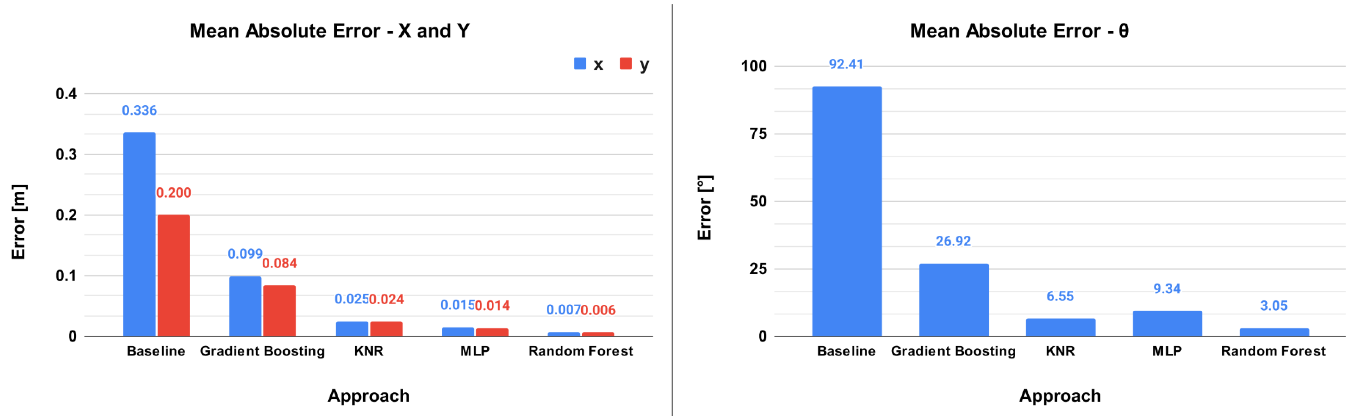
| Approach | Baseline | GB | KNR | MLP | RF | |
|---|---|---|---|---|---|---|
| MAE | x [m] | 0.336 | 0.099 | 0.025 | 0.015 | 0.007 |
| y [m] | 0.200 | 0.084 | 0.024 | 0.014 | 0.006 | |
| [°] | 92.41 | 26.92 | 6.55 | 9.34 | 3.05 | |
| RMSE | x [m] | 0.418 | 0.133 | 0.041 | 0.022 | 0.014 |
| y [m] | 0.226 | 0.109 | 0.041 | 0.021 | 0.015 | |
| [°] | 105.99 | 37.85 | 19.40 | 21.80 | 11.24 | |
| NRMSE | x | 0.303 | 0.096 | 0.030 | 0.016 | 0.010 |
| y | 0.310 | 0.149 | 0.056 | 0.030 | 0.019 | |
| 0.294 | 0.105 | 0.054 | 0.061 | 0.031 | ||
| R² | x [%] | 0.00 | 0.90 | 0.99 | 0.99 | 0.99 |
| y [%] | 0.00 | 0.77 | 0.97 | 0.99 | 0.99 | |
| [%] | 0.00 | 0.87 | 0.97 | 0.96 | 0.99 | |
| Training time [s] | - | 3302 | 28 | 1812 | 15433 | |
| Response time avg [ms] | - | 0.08 | 4.16 | 0.12 | 0.46 | |
| Grid’s Resolution | 10 mm | 5 mm | 2.5 mm | 1 mm | |
|---|---|---|---|---|---|
| Quantity of images | 8306 | 33,281 | 113,596 | 655,130 | |
| MAE | x [m] | 0.005 | 0.003 | 0.002 | 0.001 |
| y [m] | 0.005 | 0.003 | 0.002 | 0.001 | |
| [°] | 2.04 | 2.35 | 2.01 | 2.21 | |
| RMSE | x [m] | 0.008 | 0.005 | 0.003 | 0.002 |
| y [m] | 0.007 | 0.005 | 0.003 | 0.002 | |
| [°] | 8.98 | 12.46 | 10.35 | 10.60 | |
| NRMSE | x | 0.073 | 0,045 | 0.030 | 0.018 |
| y | 0.064 | 0.043 | 0.027 | 0.018 | |
| 0.025 | 0.035 | 0.029 | 0.029 | ||
| R² | x [%] | 0.95 | 0.97 | 0.99 | 0.99 |
| y [%] | 0.95 | 0.98 | 0.99 | 0.99 | |
| [%] | 0.99 | 0.99 | 0.99 | 0.99 | |
| Approach | Analytical | ML (Random Forest) | |
|---|---|---|---|
| MAE | x [m] | 0.028 | 0.022 |
| y [m] | 0.031 | 0.023 | |
| [°] | 6.00 | 7.27 | |
| RMSE | x [m] | 0.034 | 0.037 |
| y [m] | 0.037 | 0.043 | |
| [°] | 8.89 | 14.91 | |
| NRMSE | x | 0.023 | 0.025 |
| y | 0.044 | 0.051 | |
| 0.025 | 0.041 | ||
| Avg percentage Relative error | x [%] | 29.6 | 27.6 |
| y [%] | 35.9 | 22.2 | |
| [%] | 17.2 | 17.3 | |
Disclaimer/Publisher’s Note: The statements, opinions and data contained in all publications are solely those of the individual author(s) and contributor(s) and not of MDPI and/or the editor(s). MDPI and/or the editor(s) disclaim responsibility for any injury to people or property resulting from any ideas, methods, instructions or products referred to in the content. |
© 2023 by the authors. Licensee MDPI, Basel, Switzerland. This article is an open access article distributed under the terms and conditions of the Creative Commons Attribution (CC BY) license (https://creativecommons.org/licenses/by/4.0/).
Share and Cite
Klein, L.C.; Braun, J.; Mendes, J.; Pinto, V.H.; Martins, F.N.; de Oliveira, A.S.; Wörtche, H.; Costa, P.; Lima, J. A Machine Learning Approach to Robot Localization Using Fiducial Markers in RobotAtFactory 4.0 Competition. Sensors 2023, 23, 3128. https://doi.org/10.3390/s23063128
Klein LC, Braun J, Mendes J, Pinto VH, Martins FN, de Oliveira AS, Wörtche H, Costa P, Lima J. A Machine Learning Approach to Robot Localization Using Fiducial Markers in RobotAtFactory 4.0 Competition. Sensors. 2023; 23(6):3128. https://doi.org/10.3390/s23063128
Chicago/Turabian StyleKlein, Luan C., João Braun, João Mendes, Vítor H. Pinto, Felipe N. Martins, Andre Schneider de Oliveira, Heinrich Wörtche, Paulo Costa, and José Lima. 2023. "A Machine Learning Approach to Robot Localization Using Fiducial Markers in RobotAtFactory 4.0 Competition" Sensors 23, no. 6: 3128. https://doi.org/10.3390/s23063128
APA StyleKlein, L. C., Braun, J., Mendes, J., Pinto, V. H., Martins, F. N., de Oliveira, A. S., Wörtche, H., Costa, P., & Lima, J. (2023). A Machine Learning Approach to Robot Localization Using Fiducial Markers in RobotAtFactory 4.0 Competition. Sensors, 23(6), 3128. https://doi.org/10.3390/s23063128