
Two-Stage Framework for Faster Semantic Segmentation

 ,
,  ,
, 
Abstract
1. Introduction
2. Related Work
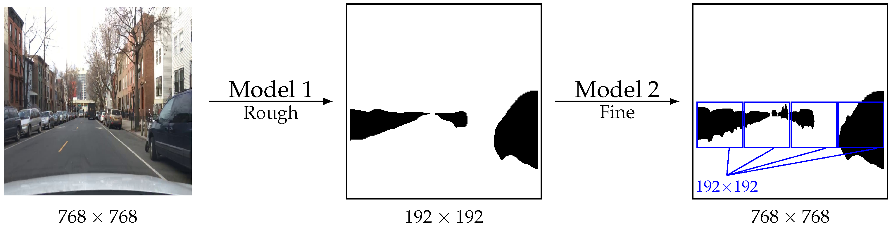
3. Method
- Step 1.
- Model 1 segments a low-resolution version of the image (line 1);
- Step 2.
- the poorly segmented image patches are identified based on the probabilities produced by Model 1 (line 2); and
- Step 3.
- Model 2 refines these patches (line 3).
| Algorithm 1: Pseudocode of the proposed method. |
Input: two models, and , and an image input x 1: 2: 3: , where and are upscale and downscale interpolations, crops the patch, for a patch by calculating the average of the uncertainty associated with the probability of each pixel, , so that highly uncertain regions correspond to those with probabilities closest to 0.5. |
3.1. Selection Method
- Random: uniform sampling.
- Weighted: Sampling is weighted by the uncertainty produced by Model 1. Shannon entropy is used as a measure of uncertainty by taking the probability map p produced by Model 1, and computing an uncertainty h score. This uncertainty is then normalized and used as the sampling probability.
- Highest: The highest uncertainty patch is always selected. While this seems to be the most obvious approach, it also removes some stochasticity and variability from the training of Model 2.
3.2. Extension
4. Experiments and Results
4.1. Datasets
4.2. Experimental Setup
4.3. Results
4.4. Ablation Studies
- The number of patches used to divide the image: There is a general reduction of quality as the number of patches is increased. However, it should be noted that this comes with a gain in latency because the more patches used, the smaller the input sizes, which means lower FLOPs, as previously detailed in Table 1.
- The sampling strategy used to select the patches during the training of Model 2: The results of varying the way that patches are selected during the training of Model 2 are based on the uncertainty produced by Model 1. The differences are not considerable, albeit always choosing the highest uncertainty patch or sampling weighted by the normalized uncertainty seem like the best strategies.
- The impact of changing the uncertainty threshold with which patches are selected for Model 2 during inference: The threshold chooses the patches from Model 1 to be refined by Model 2. The lower the uncertainty threshold, the more patches will be selected. Clearly, the more patches that are refined by Model 2, the better the final segmentation, naturally at a proportional time cost.
- Whether certain additional features from the proposal are relevant: The dashed lines illustrated in the pipeline from Figure 3 are disabled depending on whether Model 1 is used to pretrain Model 2 (fine tune) or whether an activation map is given from Model 1 to Model 2 (context). In both cases, both of these aspects of the pipeline clearly aid in improving the output quality, because disabling them lowers quality.
5. Conclusions
Author Contributions
Funding
Conflicts of Interest
References
- Long, J.; Shelhamer, E.; Darrell, T. Fully convolutional networks for semantic segmentation. In Proceedings of the IEEE Conference on Computer Vision and Pattern Recognition (CVPR), Boston, MA, USA, 7–12 June 2015; pp. 3431–3440. [Google Scholar]
- Badrinarayanan, V.; Kendall, A.; Cipolla, R. SegNet: A deep convolutional encoder-decoder architecture for image segmentation. IEEE Trans. Pattern Anal. Mach. Intell. 2017, 39, 2481–2495. [Google Scholar] [CrossRef] [PubMed]
- Ronneberger, O.; Fischer, P.; Brox, T. U-Net: Convolutional networks for biomedical image segmentation. In Proceedings of the International Conference on Medical Image Computing and Computer-Assisted Intervention (MICCAI), Munich, Germany, 5–9 October 2015; Springer: Berlin/Heidelberg, Germany, 2015; pp. 234–241. [Google Scholar]
- Chen, L.C.; Papandreou, G.; Schroff, F.; Adam, H. Rethinking atrous convolution for semantic image segmentation. arXiv 2017, arXiv:1706.05587. [Google Scholar]
- Wang, C.; Zhao, Z.; Ren, Q.; Xu, Y.; Yu, Y. Dense U-Net based on patch-based learning for retinal vessel segmentation. Entropy 2019, 21, 168. [Google Scholar] [CrossRef] [PubMed]
- Kondaveeti, H.K.; Bandi, D.; Mathe, S.E.; Vappangi, S.; Subramanian, M. A review of image processing applications based on Raspberry-Pi. In Proceedings of the 2022 8th International Conference on Advanced Computing and Communication Systems (ICACCS), Coimbatore, India, 25–26 March 2022; Volume 1, pp. 22–28. [Google Scholar]
- Fernandes, K.; Cruz, R.; Cardoso, J.S. Deep image segmentation by quality inference. In Proceedings of the 2018 International Joint Conference on Neural Networks (IJCNN), Rio de Janeiro, Brazil, 8–13 July 2018; pp. 1–8. [Google Scholar]
- Kim, J.U.; Kim, H.G.; Ro, Y.M. Iterative deep convolutional encoder-decoder network for medical image segmentation. In Proceedings of the 2017 39th Annual International Conference of the IEEE Engineering in Medicine and Biology Society (EMBC), Jeju Island, Republic of Korea, 11–15 July 2017; pp. 685–688. [Google Scholar]
- Wang, W.; Yu, K.; Hugonot, J.; Fua, P.; Salzmann, M. Recurrent U-Net for resource-constrained segmentation. In Proceedings of the IEEE/CVF International Conference on Computer Vision (ICCV), Seoul, Republic of Korea, 27 October–2 November 2019; pp. 2142–2151. [Google Scholar]
- Banino, A.; Balaguer, J.; Blundell, C. PonderNet: Learning to Ponder. In Proceedings of the 8th ICML Workshop on Automated Machine Learning (AutoML), Virtual, 23–24 July 2021. [Google Scholar]
- Silva, D.T.; Cruz, R.; Gonçalves, T.; Carneiro, D. Two-stage Semantic Segmentation in Neural Networks. In Proceedings of the Fifteenth International Conference on Machine Vision (ICMV 2022), Rome, Italy, 18–20 November 2022. [Google Scholar]
- Google AI Blog. Accurate Alpha Matting for Portrait Mode Selfies on Pixel 6. 2022. Available online: https://ai.googleblog.com/2022/01/accurate-alpha-matting-for-portrait.html (accessed on 12 February 2023).
- Miangoleh, S.M.H.; Dille, S.; Mai, L.; Paris, S.; Aksoy, Y. Boosting monocular depth estimation models to high-resolution via content-adaptive multi-resolution merging. In Proceedings of the IEEE/CVF Conference on Computer Vision and Pattern Recognition (CVPR), Nashville, TN, USA, 20–25 June 2021; pp. 9685–9694. [Google Scholar]
- Yu, Q.; Wang, H.; Kim, D.; Qiao, S.; Collins, M.; Zhu, Y.; Adam, H.; Yuille, A.; Chen, L.C. CMT-DeepLab: Clustering Mask Transformers for Panoptic Segmentation. In Proceedings of the IEEE/CVF Conference on Computer Vision and Pattern Recognition (CVPR), New Orleans, LA, USA, 18–24 June 2022; pp. 2560–2570. [Google Scholar]
- Mnih, V.; Heess, N.; Graves, A. Recurrent models of visual attention. In Proceedings of the 27th International Conference on Neural Information Processing Systems, Montreal, QC, Canada, 8–13 December 2014. [Google Scholar]
- Ba, J.; Mnih, V.; Kavukcuoglu, K. Multiple object recognition with visual attention. In Proceedings of the International Conference on Learning Representations, San Diego, CA, USA, 7–9 May 2015. [Google Scholar]
- He, K.; Zhang, X.; Ren, S.; Sun, J. Deep residual learning for image recognition. In Proceedings of the IEEE Conference on Computer Vision and Pattern Recognition, Las Vegas, NV, USA, 27–30 June 2016; pp. 770–778. [Google Scholar]
- Yu, F.; Chen, H.; Wang, X.; Xian, W.; Chen, Y.; Liu, F.; Madhavan, V.; Darrell, T. BDD100K: A Diverse Driving Dataset for Heterogeneous Multitask Learning. In Proceedings of the 2020 IEEE/CVF Conference on Computer Vision and Pattern Recognition (CVPR), Seattle, WA, USA, 13–19 June 2018. [Google Scholar]
- Alhaija, H.; Mustikovela, S.; Mescheder, L.; Geiger, A.; Rother, C. Augmented Reality Meets Computer Vision: Efficient Data Generation for Urban Driving Scenes. Int. J. Comput. Vis. (IJCV) 2018, 126, 961–972. [Google Scholar] [CrossRef]
- Kaggle. 2018 Data Science Bowl. 2018. Available online: https://www.kaggle.com/c/data-science-bowl-2018 (accessed on 12 February 2023).
- Mendonça, T.; Ferreira, P.M.; Marques, J.S.; Marcal, A.R.; Rozeira, J. PH2–A dermoscopic image database for research and benchmarking. In Proceedings of the 2013 35th Annual International Conference of the IEEE Engineering in Medicine and Biology Society (EMBC), Osaka, Japan, 3–7 July 2013; pp. 5437–5440. [Google Scholar]
- Russakovsky, O.; Deng, J.; Su, H.; Krause, J.; Satheesh, S.; Ma, S.; Huang, Z.; Karpathy, A.; Khosla, A.; Bernstein, M.; et al. ImageNet Large Scale Visual Recognition Challenge. Int. J. Comput. Vis. (IJCV) 2015, 115, 211–252. [Google Scholar] [CrossRef]
- Marcel, S.; Rodriguez, Y. Torchvision the machine-vision package of torch. In Proceedings of the 18th ACM International Conference on Multimedia, Firenze, Italy, 25–29 October 2010; pp. 1485–1488. [Google Scholar]
- Lin, T.Y.; Goyal, P.; Girshick, R.; He, K.; Dollár, P. Focal loss for dense object detection. In Proceedings of the IEEE International Conference on Computer Vision (ICCV), Venice, Italy, 22–29 October 2017; pp. 2980–2988. [Google Scholar]


| FLOPs () | ||||||
|---|---|---|---|---|---|---|
| Architecture | #Params () | |||||
| ResNet-50 * | 23.5 | 215 | 759 | 3035 | 12,142 | 48,567 |
| DeepLab v3 [4] | 42.0 | 1533 | 6132 | 24,527 | 98,107 | 392,425 |
| U-Net [3] | 73.4 | 695 | 2413 | 9653 | 38,613 | 154,452 |
| SegNet [2] | 48.4 | 594 | 1776 | 7105 | 28,421 | 113,684 |
| FCN [1] | 35.3 | 1316 | 5265 | 21,060 | 84,238 | 336,952 |
| Dataset | Category | N | Avg Res | % Fg | Example |
|---|---|---|---|---|---|
| BDD [18] | Autonomous driving | 8000 | 9.7 |  | |
| KITTI [19] | Autonomous driving | 200 | 6.6 |  | |
| BOWL [20] | Biomedical | 670 | 13.5 |  | |
| PH2 [21] | Biomedical | 200 | 31.8 |  |
| Baseline | Proposal | ||||||
|---|---|---|---|---|---|---|---|
| Architecture | Dataset | Time (s) | Time (s) | ||||
| Dice (%) | Train | Inference | Dice (%) | Train | Inference | ||
| Average | 87.6 | 181.0 | 5407.0 | 82.1 | 105.0 | 1369.9 | |
| DeepLab | BDD | 86.4 | 661.7 | 23,191.8 | 79.8 | 227.0 | 5416.6 |
| KITTI | 92.4 | 15.9 | 1363.7 | 85.6 | 11.5 | 257.5 | |
| BOWL | 87.0 | 94.0 | 4622.2 | 81.7 | 81.2 | 1772.0 | |
| PH2 | 91.9 | 15.8 | 1384.3 | 94.5 | 11.0 | 544.9 | |
| U-Net | BDD | 82.7 | 536.8 | 11,166.0 | 81.2 | 356.7 | 2338.7 |
| KITTI | 88.5 | 13.3 | 687.7 | 72.6 | 10.8 | 133.4 | |
| BOWL | 82.9 | 93.3 | 2201.5 | 83.2 | 79.7 | 966.7 | |
| PH2 | 90.5 | 13.0 | 682.3 | 91.1 | 10.4 | 251.6 | |
| SegNet | BDD | 85.9 | 529.9 | 9090.0 | 76.9 | 354.4 | 2287.3 |
| KITTI | 81.2 | 13.3 | 549.9 | 71.1 | 10.7 | 203.9 | |
| BOWL | 78.9 | 91.1 | 1868.9 | 67.1 | 79.1 | 1185.1 | |
| PH2 | 92.1 | 13.0 | 538.5 | 89.5 | 10.3 | 266.1 | |
| FCN | BDD | 86.1 | 679.2 | 21,977.2 | 79.9 | 335.5 | 3902.6 |
| KITTI | 92.9 | 16.3 | 1336.0 | 84.7 | 10.8 | 219.9 | |
| BOWL | 87.0 | 93.2 | 4507.4 | 79.4 | 80.9 | 1633.9 | |
| PH2 | 94.7 | 16.1 | 1343.8 | 94.8 | 10.3 | 538.0 | |
| (1) Dice (%) per #patches | |||||
|---|---|---|---|---|---|
| Dataset | 4 | 16 | 64 | 128 | |
| BDD | 84.4 | 79.8 | 80.1 | 68.1 | |
| KITTI | 89.3 | 85.6 | 80.3 | 53.4 | |
| BOWL | 85.5 | 81.7 | 78.9 | 75.1 | |
| PH2 | 91.5 | 94.5 | 93.1 | 88.6 | |
| (2) Dice (%) per patch selection | |||||
| Dataset | Random | Weighted | Highest | ||
| BDD | 79.3 | 79.8 | 79.9 | ||
| KITTI | 84.4 | 85.6 | 86.1 | ||
| BOWL | 80.7 | 81.7 | 81.4 | ||
| PH2 | 93.9 | 94.5 | 94.6 | ||
| (3) Dice (%) per uncertainty threshold | |||||
| Dataset | ≥1 | ≥0.75 | ≥0.5 | ≥0.25 | ≥0 |
| BDD | 75.3 | 75.5 | 76.0 | 79.8 | 84.4 |
| KITTI | 80.4 | 80.4 | 80.7 | 85.6 | 90.4 |
| BOWL | 76.5 | 76.7 | 78.0 | 81.7 | 87.2 |
| PH2 | 93.9 | 93.9 | 94.0 | 94.5 | 94.4 |
| (4) Dice (%) per disabled feature | |||||
| Dataset | Disable fine tune | Disable context | Full-featured | ||
| BDD | 77.1 | 79.0 | 79.8 | ||
| KITTI | 80.2 | 82.2 | 85.6 | ||
| BOWL | 80.4 | 78.9 | 81.7 | ||
| PH2 | 94.2 | 94.2 | 94.5 | ||
Disclaimer/Publisher’s Note: The statements, opinions and data contained in all publications are solely those of the individual author(s) and contributor(s) and not of MDPI and/or the editor(s). MDPI and/or the editor(s) disclaim responsibility for any injury to people or property resulting from any ideas, methods, instructions or products referred to in the content. |
© 2023 by the authors. Licensee MDPI, Basel, Switzerland. This article is an open access article distributed under the terms and conditions of the Creative Commons Attribution (CC BY) license (https://creativecommons.org/licenses/by/4.0/).
Share and Cite
Cruz, R.; Silva, D.T.e.; Gonçalves, T.; Carneiro, D.; Cardoso, J.S. Two-Stage Framework for Faster Semantic Segmentation. Sensors 2023, 23, 3092. https://doi.org/10.3390/s23063092
Cruz R, Silva DTe, Gonçalves T, Carneiro D, Cardoso JS. Two-Stage Framework for Faster Semantic Segmentation. Sensors. 2023; 23(6):3092. https://doi.org/10.3390/s23063092
Chicago/Turabian StyleCruz, Ricardo, Diana Teixeira e Silva, Tiago Gonçalves, Diogo Carneiro, and Jaime S. Cardoso. 2023. "Two-Stage Framework for Faster Semantic Segmentation" Sensors 23, no. 6: 3092. https://doi.org/10.3390/s23063092
APA StyleCruz, R., Silva, D. T. e., Gonçalves, T., Carneiro, D., & Cardoso, J. S. (2023). Two-Stage Framework for Faster Semantic Segmentation. Sensors, 23(6), 3092. https://doi.org/10.3390/s23063092