
FPGA-Based Vehicle Detection and Tracking Accelerator


Abstract
1. Introduction
- We trained the YOLOv3 and YOLOv3-tiny networks using the UA-DETRAC dataset [17]. Then, we incorporate the dynamic threshold structured pruning strategy based on binary search and the dynamic INT16 fixed-point quantization algorithm to compress the model.
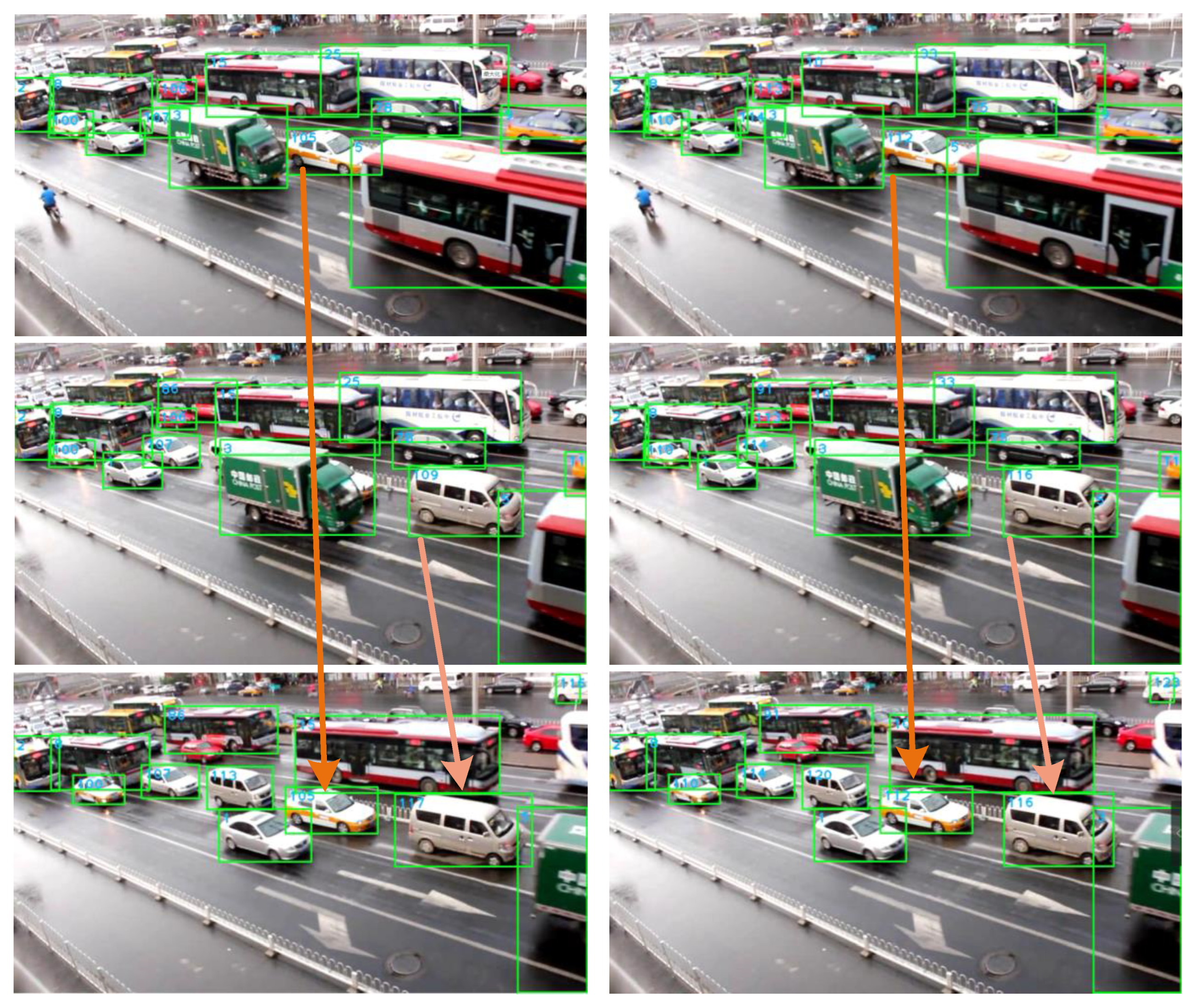
- A reidentification dataset was generated based on the UA-DETRAC dataset and used to train the appearance feature extraction network of the Deepsort algorithm with a modified input size to improve the vehicle tracking performance.
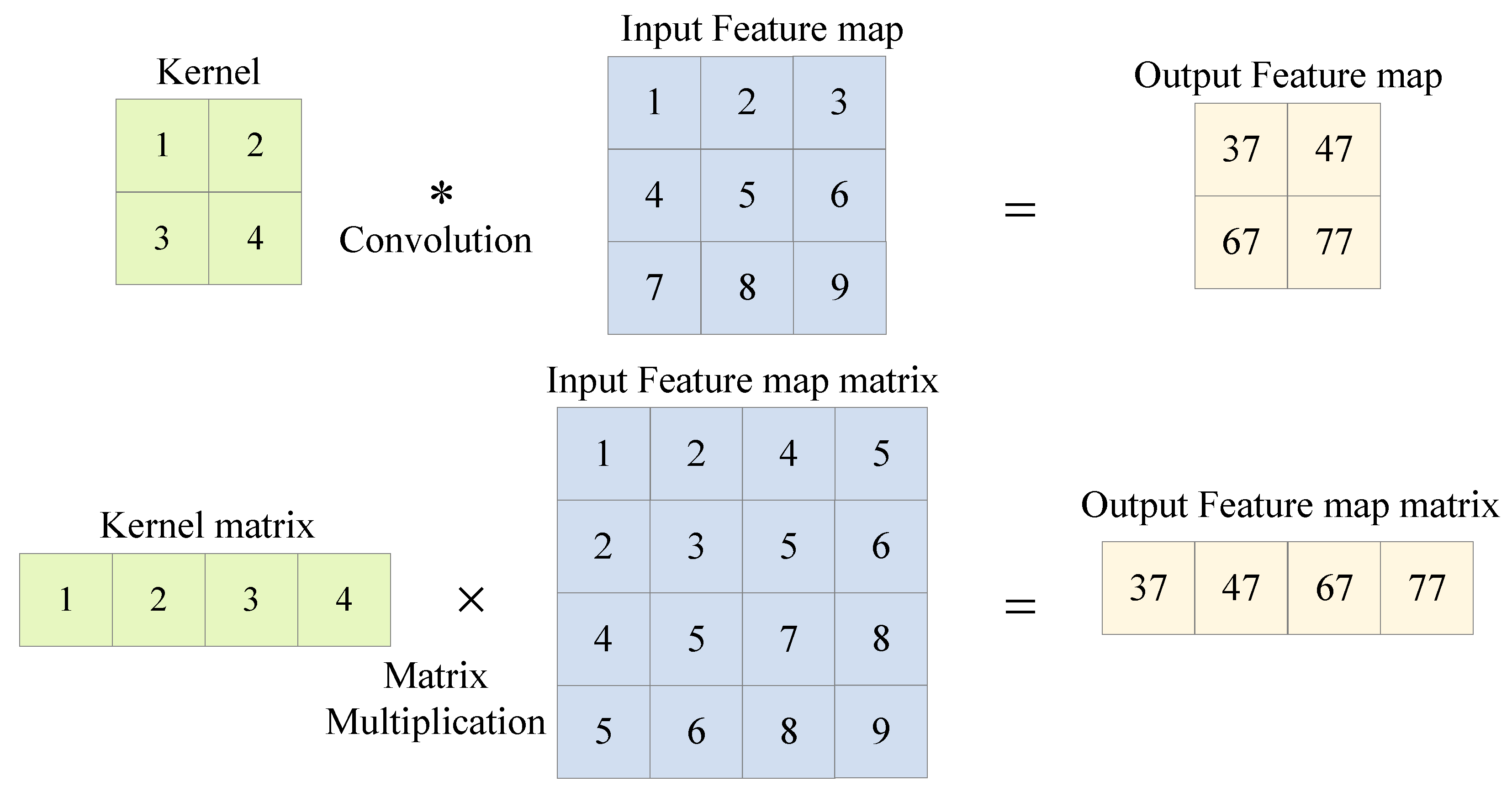
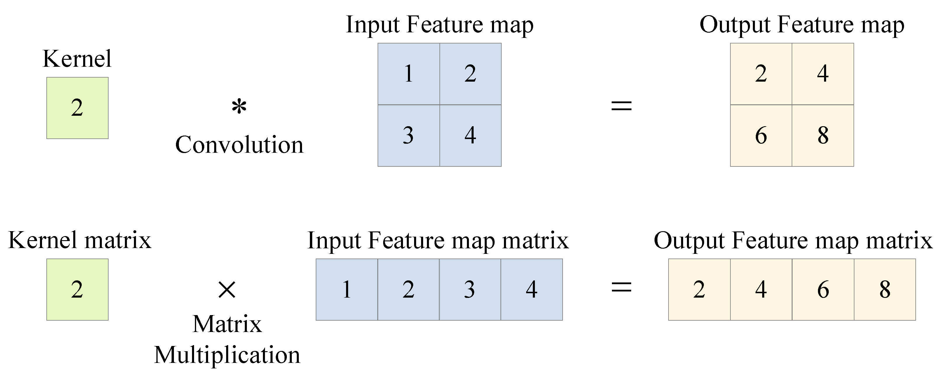
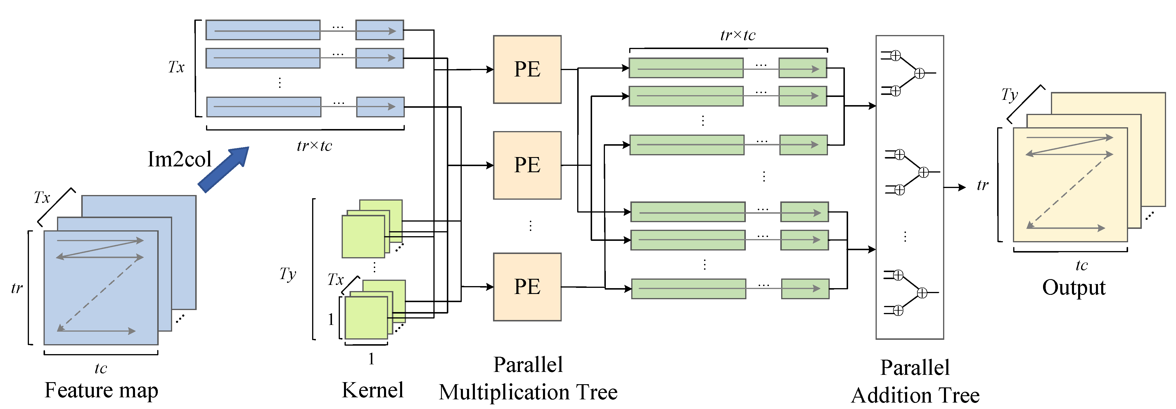
- We designed and implemented a vehicle detector based on an FPGA using high level synthesis (HLS) technology. At the hardware level, optimization techniques such as the Im2col+GEMM and Winograd algorithms, parameter rearrangement, and multichannel transmission are adopted to improve the computational throughput and balance the resource occupancy and power consumption. Compared with the other related work, vehicle detection performance with higher precision and higher throughput is realized with lower power consumption.
- Our design adopts a loosely coupled architecture, which can flexibly switch between the two detection models by changing the memory management module, optimizing the balance between the software flexibility and high computing efficiency of the dedicated chips.
2. Background and Related Work
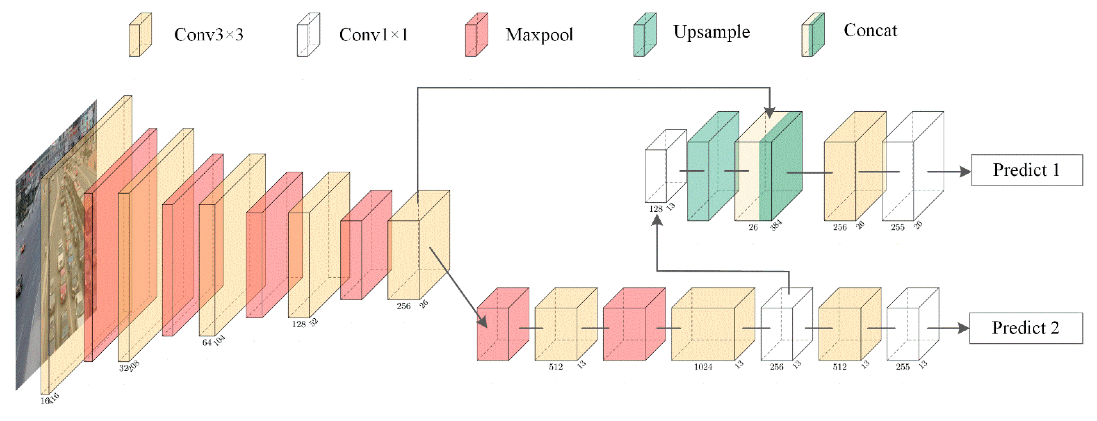
2.1. YOLO
2.2. Deepsort
2.3. Simplification of the DNN
2.4. CNN Accelerator Based on an FPGA
3. Optimization and Implementation of the Vehicle Detector
3.1. Model Compression
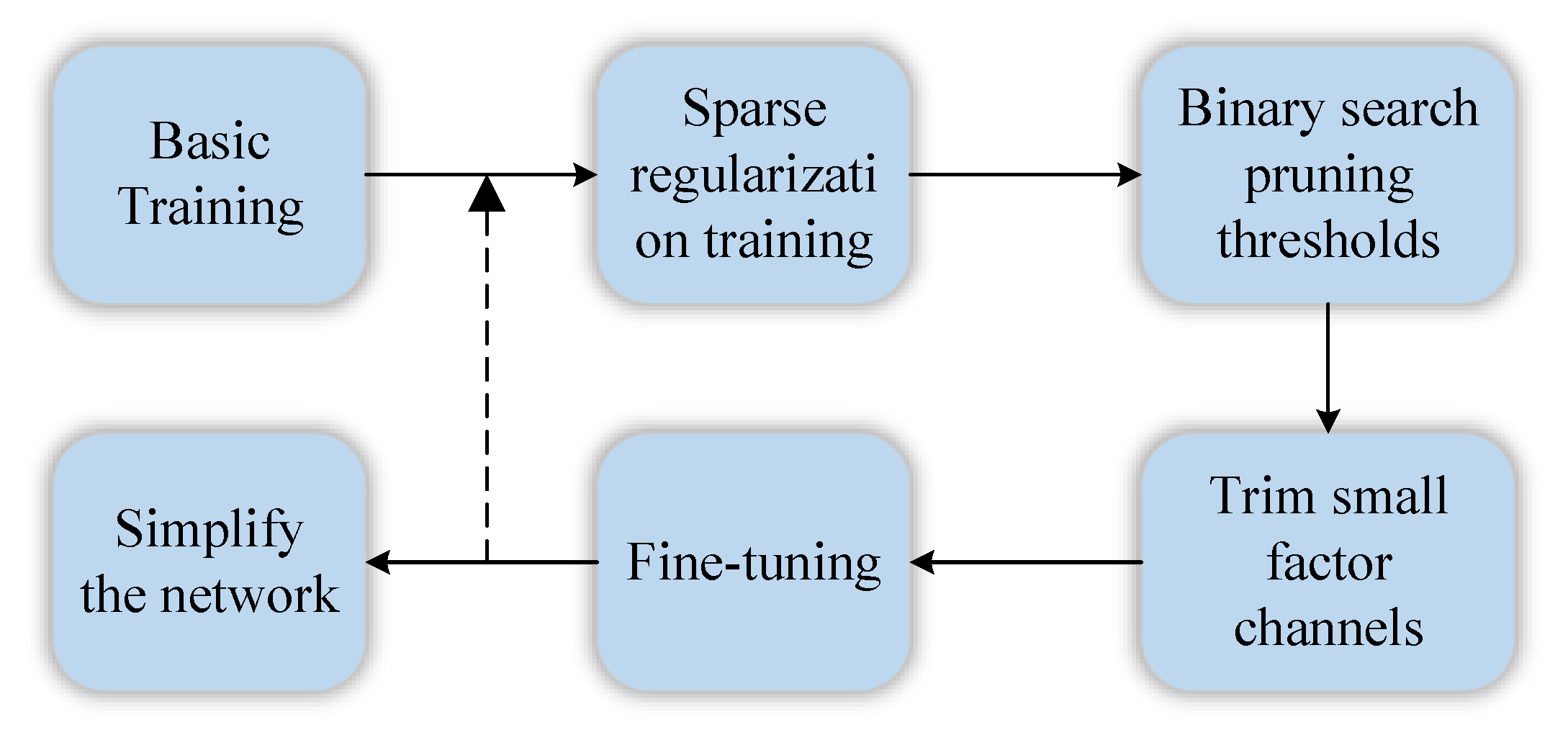
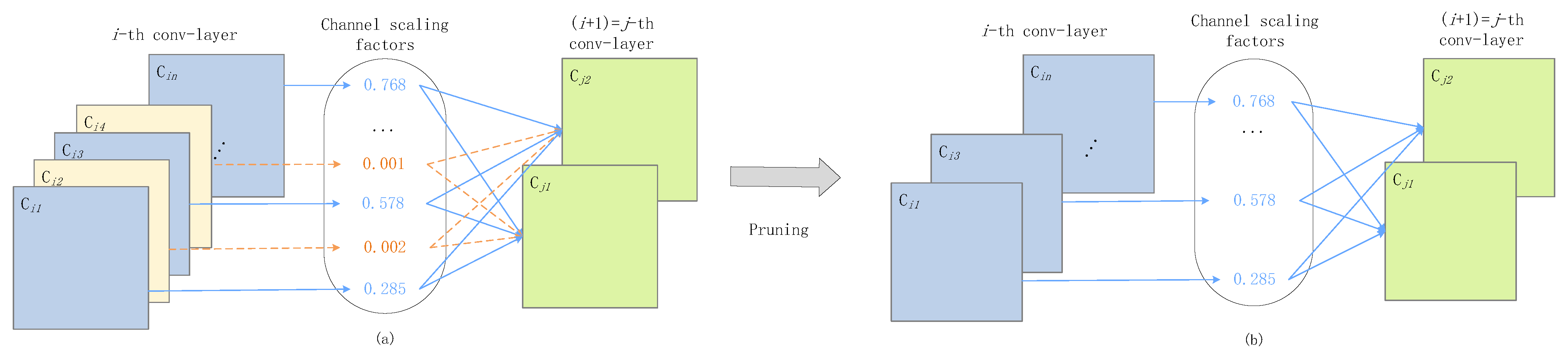
3.1.1. Structured Pruning Based on Dynamic Threshold of Binary Search
3.1.2. Dynamic 16-bit Fixed-Point Quantization
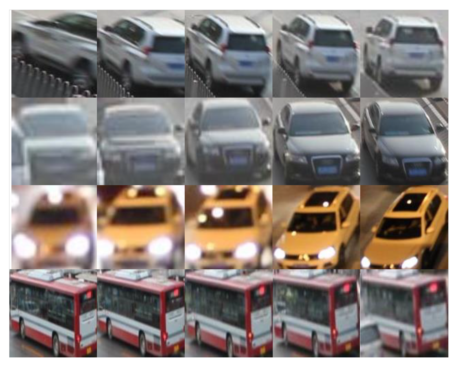
3.2. Self-Generated REID-UADETRAC Dataset
3.3. Overview of the Accelerator Architecture
3.4. Strategies of Memory Optimization
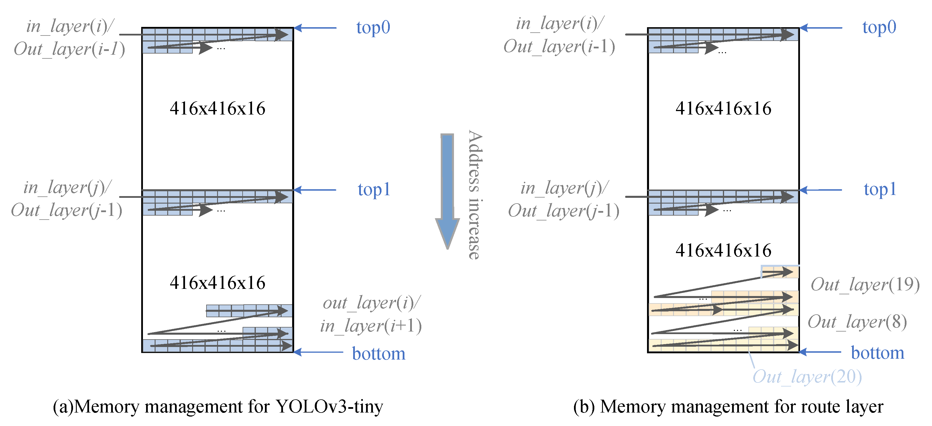
3.4.1. Model Configurability and Memory Interlayer Multiplexing
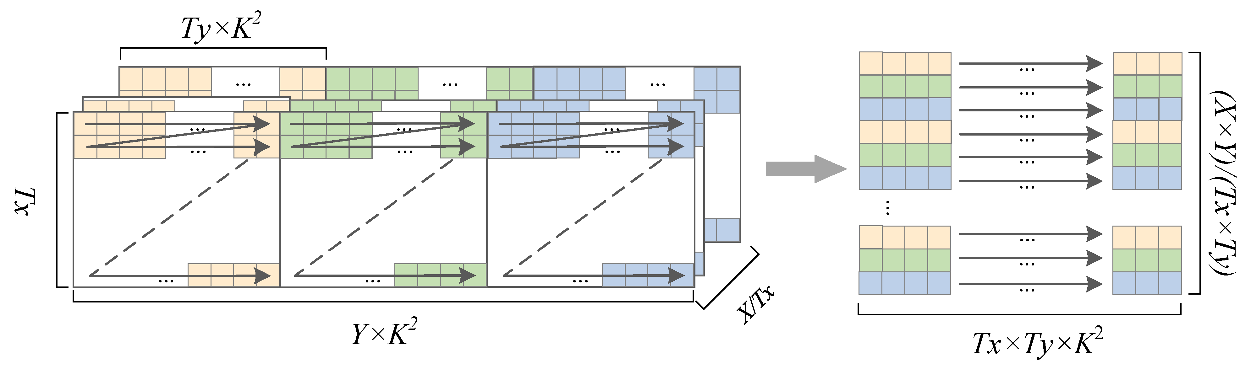
3.4.2. Parameter Rearrangement in Memory
3.4.3. Multichannel Transmission
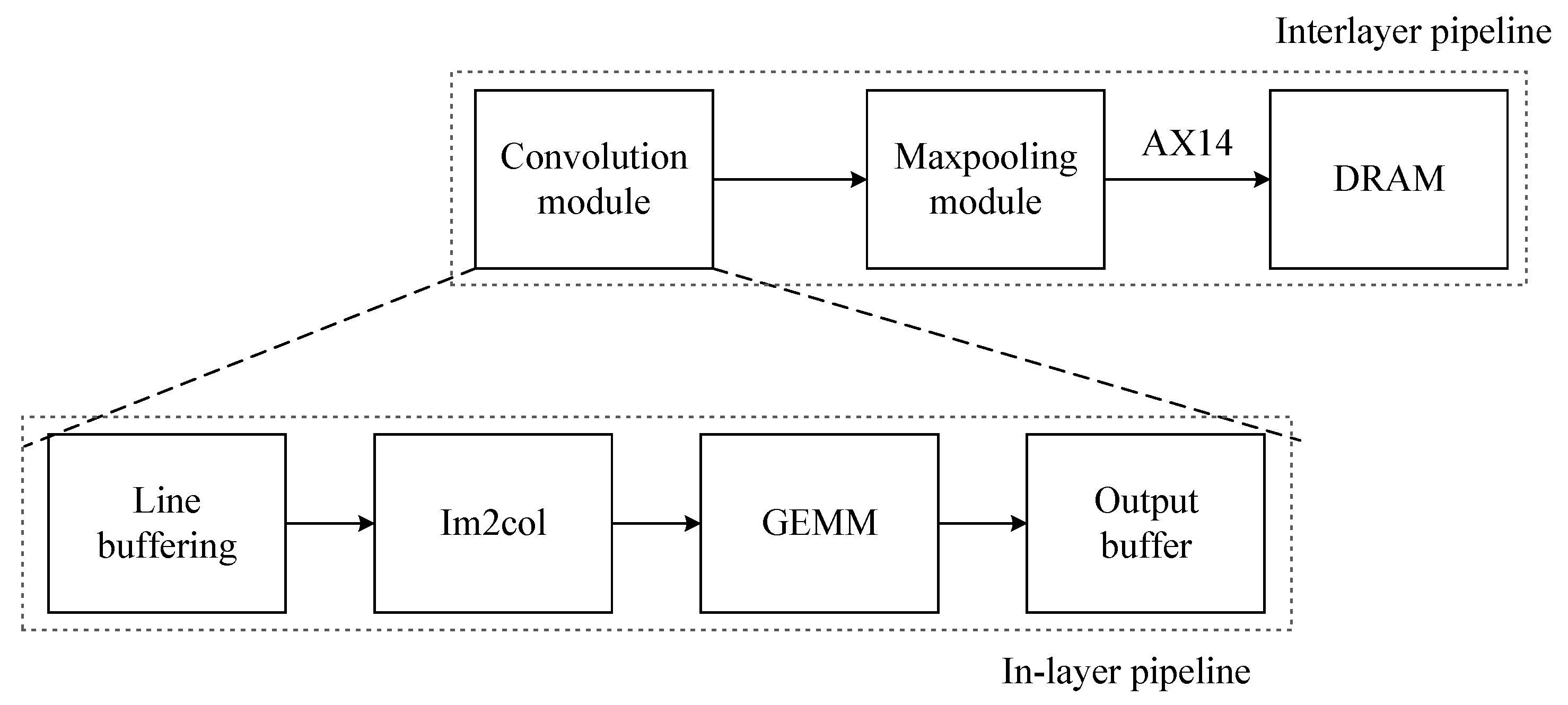
3.4.4. Multi-Level Pipeline Optimization
3.5. Strategies of Computational Optimization
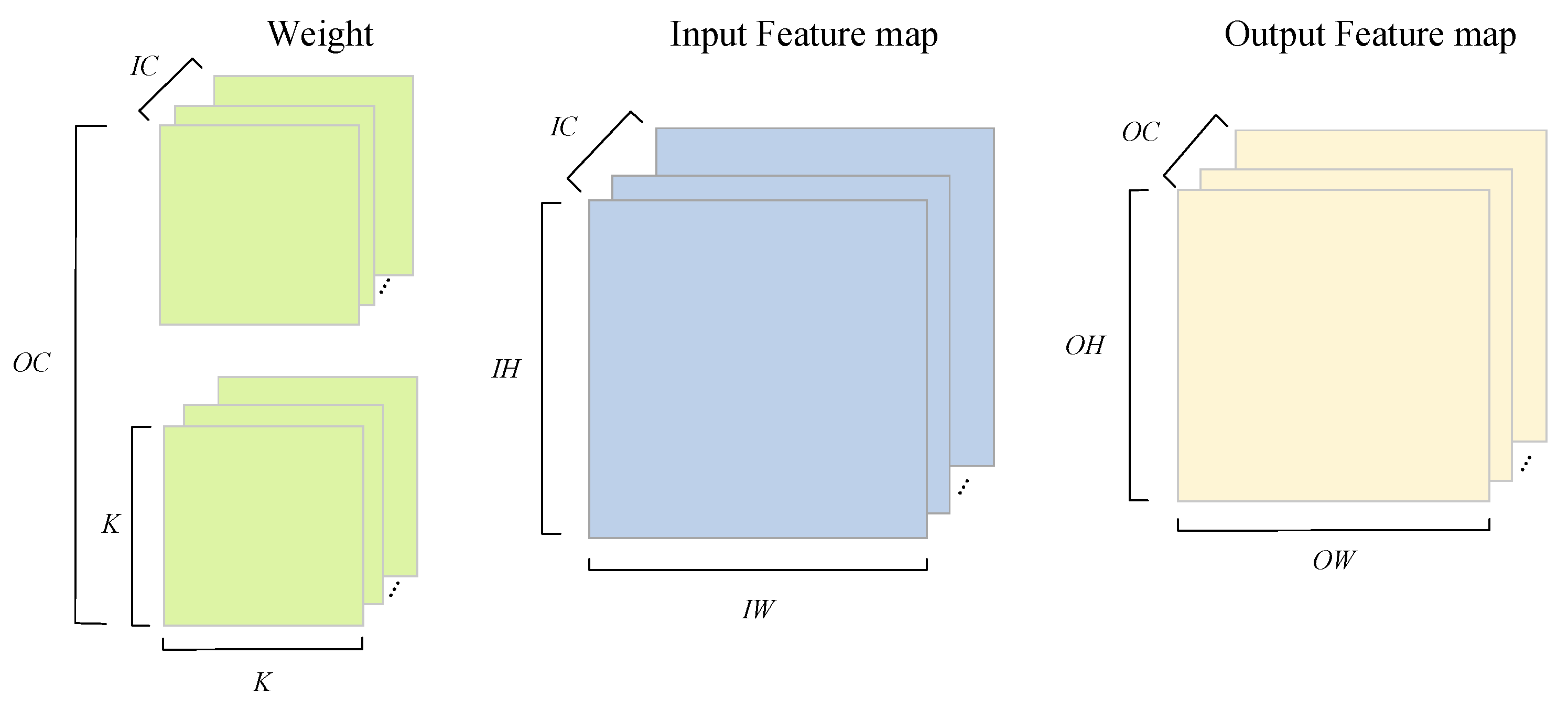
Multiscale Convolution Acceleration Engines
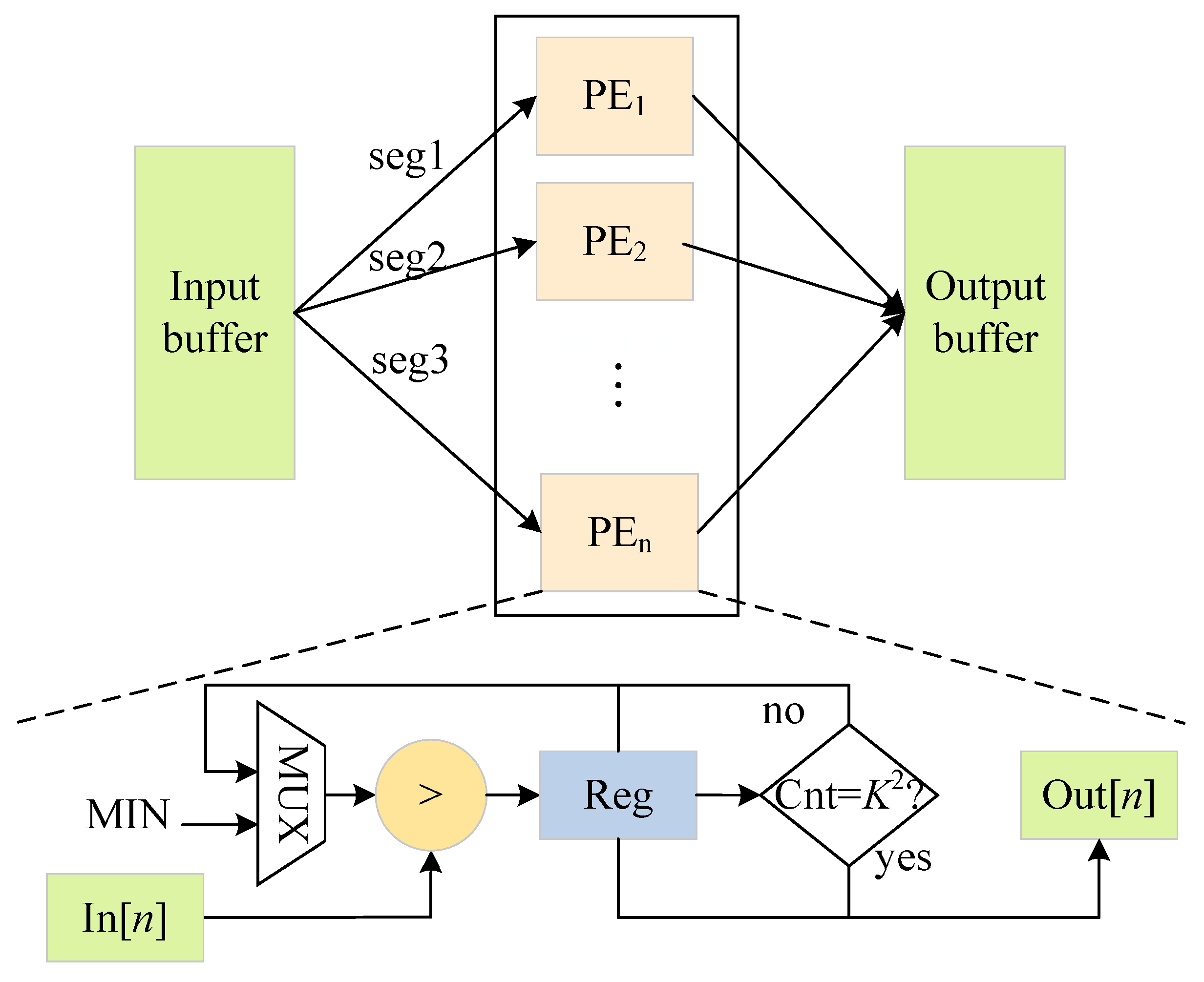
3.6. Max-Pooling and Upsampling Parallel Optimization
Fused Convolution and Batch Normalization Computation
4. Experiments
4.1. Experimental Setup
4.2. Dataset and Model Training
4.3. RE-ID Deepsort
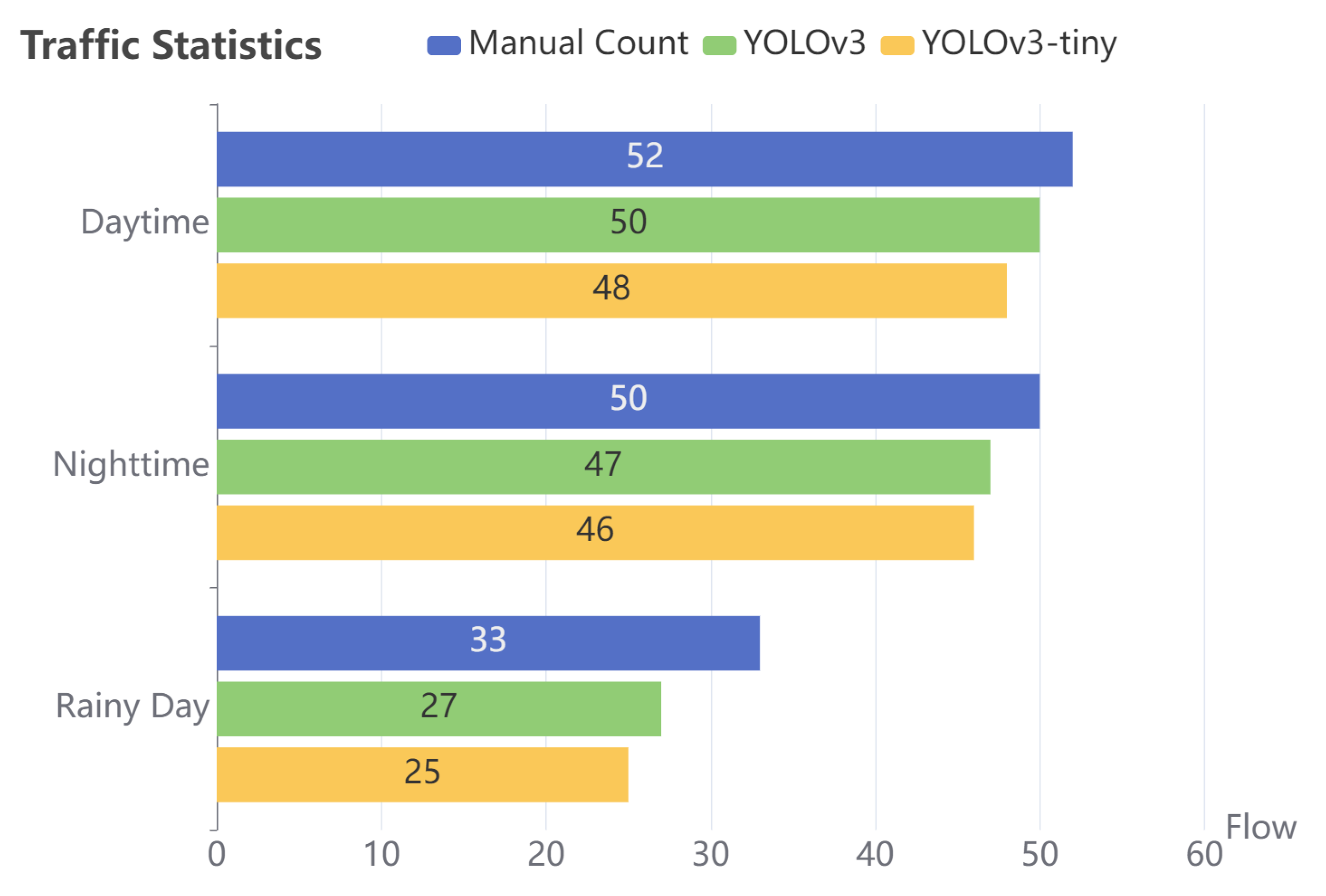
4.4. Comparison and Discussion
4.5. Scalability Discussion
5. Conclusions and Future Work
Author Contributions
Funding
Institutional Review Board Statement
Informed Consent Statement
Data Availability Statement
Conflicts of Interest
References
- Jan, B.; Farman, H.; Khan, M.; Talha, M.; Din, I.U. Designing a Smart Transportation System: An Internet of Things and Big Data Approach. IEEE Wirel. Commun. 2019, 26, 73–79. [Google Scholar] [CrossRef]
- Lin, J.; Yu, W.; Yang, X.; Zhao, P.; Zhang, H.; Zhao, W. An Edge Computing Based Public Vehicle System for Smart Transportation. IEEE Trans. Veh. Technol. 2020, 69, 12635–12651. [Google Scholar] [CrossRef]
- Wang, S.; Djahel, S.; Zhang, Z.; McManis, J. Next Road Rerouting: A Multiagent System for Mitigating Unexpected Urban Traffic Congestion. IEEE Trans. Intell. Transp. Syst. 2016, 17, 2888–2899. [Google Scholar] [CrossRef]
- Tseng, Y.-T.; Ferng, H.-W. An Improved Traffic Rerouting Strategy Using Real-Time Traffic Information and Decisive Weights. IEEE Trans. Veh. Technol. 2021, 70, 9741–9751. [Google Scholar] [CrossRef]
- Heitz, D.; Mémin, E.; Schnörr, C. Variational fluid flow measurements from image sequences: Synopsis and perspectives. Exp. Fluids 2010, 48, 369–393. [Google Scholar] [CrossRef]
- Zivkovic, Z.; van der Heijden, F. Efficient adaptive density estimation per image pixel for the task of background subtraction. Pattern Recognit. Lett. 2006, 27, 773–780. [Google Scholar] [CrossRef]
- Wang, G.; Wu, J.; Xu, T.; Tian, B. 3D Vehicle Detection With RSU LiDAR for Autonomous Mine. IEEE Trans. Veh. Technol. 2021, 70, 344–355. [Google Scholar] [CrossRef]
- Nguyen, D.T.; Nguyen, T.N.; Kim, H.; Lee, H.-J. A High-Throughput and Power-Efficient FPGA Implementation of YOLO CNN for Object Detection. IEEE Trans. Very Large Scale Integr. (VLSI) Syst. 2019, 27, 1861–1873. [Google Scholar] [CrossRef]
- Girshick, R.; Donahue, J.; Darrell, T.; Malik, J. Region-Based Convolutional Networks for Accurate Object Detection and Segmentation. IEEE Trans. Pattern Anal. Mach. Intell. 2016, 38, 142–158. [Google Scholar] [CrossRef]
- Ren, S.; He, K.; Girshick, R.; Sun, J. Faster R-CNN: Towards Real-Time Object Detection with Region Proposal Networks. Adv. Neural Inf. Process. Syst. 2015, 28. Available online: https://proceedings.neurips.cc/paper/2015/hash/14bfa6bb14875e45bba028a21ed38046-Abstract.html (accessed on 1 January 2023). [CrossRef]
- Liu, W.; Anguelov, D.; Erhan, D.; Szegedy, C.; Reed, S.; Fu, C.Y.; Berg, A.C. SSD: Single Shot MultiBox Detector. In Computer Vision–ECCV 2016: 14th European Conference, Amsterdam, The Netherlands, 11–14 October 2016, Proceedings, Part I 14; Springer International Publishing: Cham, Switzerland, 2016; pp. 21–37. [Google Scholar] [CrossRef]
- Redmon, J.; Divvala, S.; Girshick, R.; Farhadi, A. You Only Look Once: Unified, Real-Time Object Detection. In Proceedings of the IEEE Conference on Computer Vision and Pattern Recognition (CVPR), Las Vegas, NV, USA, 26 June–1 July 2016; pp. 779–788. [Google Scholar]
- Redmon, J.; Farhadi, A. YOLO9000: Better, Faster, Stronger. In Proceedings of the IEEE Conference on Computer Vision and Pattern Recognition (CVPR), Honolulu, HI, USA, 21–26 July 2017; pp. 7263–7271. [Google Scholar]
- Pei, S.; Wang, X. Research on FPGA-Accelerated Computing Model of YOLO Detection Network. Small Microcomput. Syst. Available online: https://kns.cnki.net/kcms/detail/21.1106.TP.20210906.1741.062.html (accessed on 1 January 2023).
- Zhao, M.; Peng, J.; Yu, S.; Liu, L.; Wu, N. Exploring Structural Sparsity in CNN via Selective Penalty. IEEE Trans. Circuits Syst. Video Technol. 2022, 32, 1658–1666. [Google Scholar] [CrossRef]
- Nguyen, D.T.; Kim, H.; Lee, H.-J. Layer-Specific Optimization for Mixed Data Flow With Mixed Precision in FPGA Design for CNN-Based Object Detectors. IEEE Trans. Circuits Syst. Video Technol. 2021, 31, 2450–2464. [Google Scholar] [CrossRef]
- Wen, L.; Du, D.; Cai, Z.; Lei, Z.; Chang, M.-C.; Qi, H.; Lim, J.; Yang, M.-H.; Lyu, S. UA-DETRAC: A new benchmark and protocol for multi-object detection and tracking. Comput. Vis. Image Underst. 2020, 193, 102907. [Google Scholar] [CrossRef]
- Wojke, N.; Bewley, A.; Paulus, D. Simple online and realtime tracking with a deep association metric. In Proceedings of the 2017 IEEE International Conference on Image Processing (ICIP), Beijing, China, 17–20 September 2017; pp. 3645–3649. [Google Scholar] [CrossRef]
- Wright, M.B. Speeding up the hungarian algorithm. Comput. Oper. Res. 1990, 17, 95–96. [Google Scholar] [CrossRef]
- De Maesschalck, R.; Jouan-Rimbaud, D.; Massart, D.L. The Mahalanobis distance. Chemom. Intell. Lab. Syst. 2000, 50, 1–18. [Google Scholar] [CrossRef]
- Han, S.; Pool, J.; Tran, J.; Dally, W. Learning both Weights and Connections for Efficient Neural Network. Adv. Neural Inf. Process. Syst. 2015, 28. Available online: https://proceedings.neurips.cc/paper/2015/hash/ae0eb3eed39d2bcef4622b2499a05fe6-Abstract.html (accessed on 1 January 2023).
- Li, H.; Kadav, A.; Durdanovic, I.; Samet, H.; Graf, H.P. Pruning Filters for Efficient ConvNets. arXiv 2017, arXiv:1608.08710. [Google Scholar]
- Yang, T.-J.; Howard, A.; Chen, B.; Zhang, X.; Go, A.; Sandler, M.; Sze, V.; Adam, H. NetAdapt: Platform-Aware Neural Network Adaptation for Mobile Applications. In Proceedings of the European Conference on Computer Vision (ECCV), Munich, Germany, 8–14 September 2018; pp. 285–300. [Google Scholar]
- Liu, Z.; Li, J.; Shen, Z.; Huang, G.; Yan, S.; Zhang, C. Learning Efficient Convolutional Networks Through Network Slimming. In Proceedings of the IEEE International Conference on Computer Vision, Venice, Italy, 27–29 October 2017; pp. 2736–2744. [Google Scholar]
- Liu, Z.; Sun, M.; Zhou, T.; Huang, G.; Darrell, T. Rethinking the Value of Network Pruning. arXiv 2019, arXiv:1810.05270. [Google Scholar]
- Qiu, J.; Wang, J.; Yao, S.; Guo, K.; Li, B.; Zhou, E.; Yu, J.; Tang, T.; Xu, N.; Song, S.; et al. Going Deeper with Embedded FPGA Platform for Convolutional Neural Network. In Proceedings of the 2016 ACM/SIGDA International Symposium on Field-Programmable Gate Arrays, New York, NY, USA, 21–23 February 2016; pp. 26–35. [Google Scholar] [CrossRef]
- Cardarilli, G.C.; Di Nunzio, L.; Fazzolari, R.; Giardino, D.; Matta, M.; Patetta, M.; Re, M.; Spanò, S. Approximated computing for low power neural networks. TELKOMNIKA (Telecommun. Comput. Electron. Control.) 2019, 17, 1236–1241. [Google Scholar] [CrossRef]
- Ma, Y.; Cao, Y.; Vrudhula, S.; Seo, J. Optimizing Loop Operation and Dataflow in FPGA Acceleration of Deep Convolutional Neural Networks. In Proceedings of the 2017 ACM/SIGDA International Symposium on Field-Programmable Gate Arrays, Monterey, CA, USA, 22–24 February 2017; pp. 45–54. [Google Scholar] [CrossRef]
- Zhang, C.; Li, P.; Sun, G.; Guan, Y.; Xiao, B.; Cong, J. Optimizing FPGA-based Accelerator Design for Deep Convolutional Neural Networks. In Proceedings of the 2015 ACM/SIGDA International Symposium on Field-Programmable Gate Arrays, New York, NY, USA, 22–24 February 2015; pp. 161–170. [Google Scholar] [CrossRef]
- Lu, L.; Liang, Y.; Xiao, Q.; Yan, S. Evaluating Fast Algorithms for Convolutional Neural Networks on FPGAs. In Proceedings of the 2017 IEEE 25th Annual International Symposium on Field-Programmable Custom Computing Machines (FCCM), Napa, CA, USA, 30 April–2 May 2017; pp. 101–108. [Google Scholar] [CrossRef]
- Lu, L.; Liang, Y. SpWA: An efficient sparse winograd convolutional neural networks accelerator on FPGAs. In Proceedings of the 55th Annual Design Automation Conference, San Francisco, CA, USA, 24–29 June 2018; pp. 1–6. [Google Scholar] [CrossRef]
- Bao, C.; Xie, T.; Feng, W.; Chang, L.; Yu, C. A Power-Efficient Optimizing Framework FPGA Accelerator Based on Winograd for YOLO. IEEE Access 2020, 8, 94307–94317. [Google Scholar] [CrossRef]
- Wang, Z.; Xu, K.; Wu, S.; Liu, L.; Liu, L.; Wang, D. Sparse-YOLO: Hardware/Software Co-Design of an FPGA Accelerator for YOLOv2. IEEE Access 2020, 8, 116569–116585. [Google Scholar] [CrossRef]
- McFarland, M.C.; Parker, A.C.; Camposano, R. The high-level synthesis of digital systems. Proc. IEEE 1990, 78, 301–318. [Google Scholar] [CrossRef]
- Yeom, S.-K.; Seegerer, P.; Lapuschkin, S.; Binder, A.; Wiedemann, S.; Müller, K.R.; Samek, W. Pruning by explaining: A novel criterion for deep neural network pruning. Pattern Recognit. 2021, 115, 107899. [Google Scholar] [CrossRef]
- Shan, L.; Zhang, M.; Deng, L.; Gong, G. A Dynamic Multi-precision Fixed-Point Data Quantization Strategy for Convolutional Neural Network. In Computer Engineering and Technology: 20th CCF Conference, NCCET 2016, Xi’an, China, August 10–12, 2016, Revised Selected Papers; Springer: Singapore, 2016; pp. 102–111. [Google Scholar] [CrossRef]
- Chen, C.; Xia, J.; Yang, W.; Li, K.; Chai, Z. A PYNQ-compliant Online Platform for Zynq-based DNN Developers. In Proceedings of the 2019 ACM/SIGDA International Symposium on Field-Programmable Gate Arrays, New York, NY, USA, 24–26 February 2019; p. 185. [Google Scholar] [CrossRef]
- Qi, Y.; Zhou, X.; Li, B.; Zhou, Q. FPGA-based CNN image recognition acceleration and optimization. Comput. Sci. 2021, 48, 205–212. [Google Scholar] [CrossRef]
- Liu, Z.-G.; Whatmough, P.N.; Mattina, M. Systolic Tensor Array: An Efficient Structured-Sparse GEMM Accelerator for Mobile CNN Inference. IEEE Comput. Archit. Lett. 2020, 19, 34–37. [Google Scholar] [CrossRef]
- Lavin, A.; Gray, S. Fast Algorithms for Convolutional Neural Networks. In Proceedings of the IEEE Conference on Computer Vision and Pattern Recognition (CVPR), Las Vegas, NV, USA, 27–30 June 2016; pp. 4013–4021. [Google Scholar]
- Ji, Z.; Zhang, X.; Wei, Z.; Li, J.; Wei, J. A tile-fusion method for accelerating Winograd convolutions. Neurocomputing 2021, 460, 9–19. [Google Scholar] [CrossRef]
- Adiono, T.; Putra, A.; Sutisna, N.; Syafalni, I.; Mulyawan, R. Low Latency YOLOv3-Tiny Accelerator for Low-Cost FPGA Using General Matrix Multiplication Principle. IEEE Access 2021, 9, 141890–141913. [Google Scholar] [CrossRef]
- Ioffe, S.; Szegedy, C. Batch Normalization: Accelerating Deep Network Training by Reducing Internal Covariate Shift. In Proceedings of the 32nd International Conference on Machine Learning, Lille, France, 7–9 July 2015; pp. 448–456. [Google Scholar]
- Milan, A.; Leal-Taixe, L.; Reid, I.; Roth, S.; Schindler, K. MOT16: A Benchmark for Multi-Object Tracking. arXiv 2016, arXiv:1603.00831. [Google Scholar]
- Taheri Tajar, A.; Ramazani, A.; Mansoorizadeh, M. A lightweight Tiny-YOLOv3 vehicle detection approach. J. -Real-Time Image Process. 2021, 18, 2389–2401. [Google Scholar] [CrossRef]
- Ding, C.; Wang, S.; Wang, N.; Xu, K.; Wang, Y.; Liang, Y. REQ-YOLO: A resource-aware, efficient quantization framework for object detection on FPGAs. In Proceedings of the 2019 ACM/SIGDA International Symposium on Field-Programmable Gate Arrays, Seaside, CA, USA, 24–26 February 2019; pp. 33–42. [Google Scholar]


| Variables | Meaning |
|---|---|
| The parameter for regulating the effect of the spatial Mahalanobis distance and visual distance on the cost function. | |
| The state vector of the i-th prediction frame. | |
| The covariance matrix of the average tracking results between the detection frame and track i. | |
| Detection box j. | |
| The appearance descriptor extracted from detection box j. | |
| The last 100 appearance descriptor sets associated with track i. |
| Symbol | Meaning |
|---|---|
| I | The input feature map. |
| W | The weights of the convolution layer. |
| B | The bias of the convolution layer. |
| O | The output feature map. |
| The height of the input feature map. | |
| The width of the input feature map. | |
| The number of input channels. | |
| K | The kernel size. |
| The height of the output feature map. | |
| The width of the output feature map. | |
| The number of output channels. | |
| The padding. | |
| S | The stride. |
| Parallelism of multiply-add operations on input feature maps. | |
| Parallelism of multiply-add operations on output feature maps. |
| Symbol | Meaning |
|---|---|
| The output of the feature map after batch normalization. | |
| The parameter that controls the variance of . | |
| The variance of O. | |
| A small constant used to prevent numerical error. | |
| O | The output of the feature map. |
| The estimate of the mean of O. | |
| The parameters that control the mean of . |
| Model | Pruning Rate | AP@0.5 | Model Size (MB) | Parameters () | BFLOPs |
|---|---|---|---|---|---|
| YOLOv3 | 0 | 0.671 | 235.06 | 61523 | 65.864 |
| YOLOv3 | 85% | 0.711 | 33.55 | 8719 | 19.494 |
| YOLOv3-tiny | 0 | 0.625 | 33.10 | 8670 | 5.444 |
| YOLOv3-tiny | 85% | 0.625 | 1.02 | 267 | 1.402 |
| YOLOv3-tiny | 85% + 30% | 0.599 | 0.59 | 69 | 0.735 |
| Model | Number of Vehicles Detected |
|---|---|
| YOLOv3 | 27 |
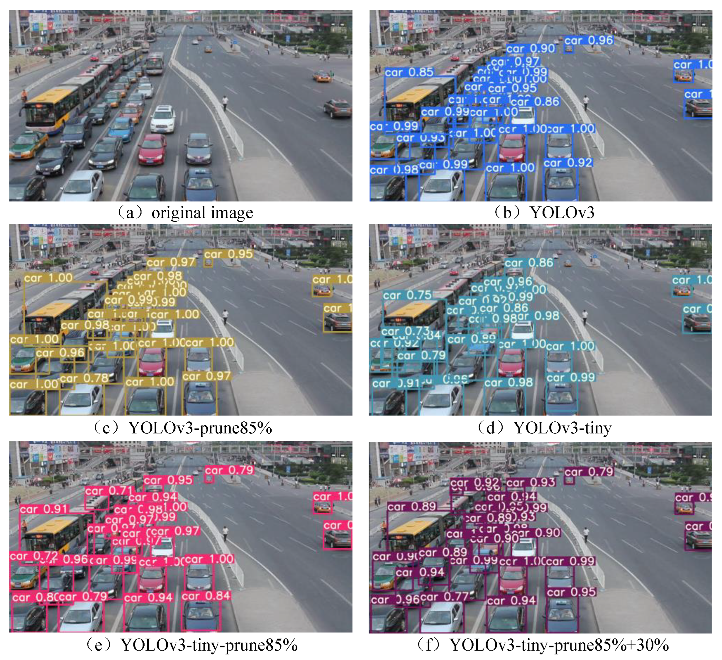
| YOLOv3-prune85% | 27 |
| YOLOv3-tiny | 24 |
| YOLOv3-tiny-prune85% | 24 |
| YOLOv3-tiny-prune85%+30% | 26 |
| Model | Video Stream | IDF1↑ | IDP↑ | IDR↑ | FP↓ | FN↓ | IDs↓ | MOTA↑ | MOTP↓ |
|---|---|---|---|---|---|---|---|---|---|
| Deepsort | MVI_40701 | 76.4% | 82.5% | 71.1% | 1515 | 3706 | 53 | 66.8% | 0.118 |
| RE-ID Deepsort | 79.6% | 86.4% | 76.2% | 1452 | 3686 | 27 | 67.5% | 0.117 | |
| Deepsort | MVI_40771 | 69.3% | 74.5% | 66.2% | 2409 | 2409 | 49 | 65.2% | 0.153 |
| RE-ID Deepsort | 80.6% | 87.2% | 75.0% | 1015 | 2348 | 13 | 69.6% | 0.155 | |
| Deepsort | MVI_40863 | 55.2% | 80.6% | 42.0% | 2076 | 17746 | 51 | 39.2% | 0.138 |
| RE-ID Deepsort | 56.1% | 82.0% | 42.6% | 2037 | 17382 | 35 | 40.5% | 0.138 |
| Item | Platform | CNN Model | Operation (GOP) | Throughput (fps) | Full Power (W) | Efficiency (GOPS/W) | Cost Efficiency (GOPS/$) |
|---|---|---|---|---|---|---|---|
| Baseline1 | CPU AMD R75800H | YOLOv3-tiny | 0.735 | 10.01 | 45 | 0.16 | 1.96 |
| Baseline2 | GeForce RTX 2060 | YOLOv3-tiny | 0.735 | 112.87 | 160 | 0.52 | 16.58 |
| Baseline3 | XCZU9EG-FFVB1156 | yolov3-adas-pruned-0.9 | 5.5 | 84.1 | - | 3.71 | 4.16 |
| Ref [45] | Nvidia Jetson Nano | YOLOv3-tiny | 1.81 | 17 | 10 | 3.08 | 24.62 |
| This work | Zynq-7000 | YOLOv3-tiny | 0.735 | 91.65 | 12.51 | 5.43 | 46.51 |
| Item | Ref [14] | Ref [37] | Ref [33] | Ref [46] | This Work | ||||
|---|---|---|---|---|---|---|---|---|---|
| Basic information introduction | |||||||||
| Platform | ZYNQ XC7Z020 | Zedboard | Arria-10GX1150 | Virtex-7: XC7VX690T-2 | Zynq-7000 | ||||
| Precision | Fixed-16 | Fixed-16 | Int8 | Float-32 | Float-32 | Fixed-16 | |||
| CNN Model | YOLOv2 | YOLOv2 | YOLOv2-tiny | YOLOv2 | YOLOv2-tiny | YOLOv3 | YOLOv3-tiny | YOLOv3 | YOLOv3-tiny |
| Dataset | COCO | COCO | VOC | VOC | UA-DETRAC | ||||
| Hardware resource consumption | |||||||||
| BRAM | 87.5 | 88 | 96% | 1320 | 98.5 (19.7%) | 132.5 (26.5%) | |||
| DSPs | 150 | 153 | 6% | 3456 | 301 (33.8%) | 144 (16.2%) | |||
| LUTs | 36 576 | 37 342 | 45% | 637 560 | 38 336 (22.3%) | 38 228 (22.2%) | |||
| FFs | 43 940 | 35 785 | 717 660 | 62 988 (18.3%) | 42 853 (12.5%) | ||||
| Performance comparison | |||||||||
| mAP | 0.481 | 0.481 | - | 0.744 | 0.548 | 0.711 | 0.599 | 0.711 | 0.599 |
| Operations (GOP) | 29.47 | 29.47 | 5.14 | 4.2 | 1.24 | 19.494 | 0.735 | 19.494 | 0.735 |
| Freq (MHz) | 150 | 150 | 204 | 200 | 210 | 230 | |||
| Performance (GOP/s) | 64.91 | 30.15 | 21.97 | 182.36 | 389.90 | 41.39 | 43.47 | 63.51 | 67.91 |
| Throughput(fps) | 2.20 | 1.02 | 4.27 | 61.90 | 314.2 | 2.12 | 59.14 | 3.23 | 91.65 |
| Efficiency comparison | |||||||||
| Cost Efficiency (GOPS/$×) | 44.45 | 20.65 | 15.05 | 17.49 | 46.75 | 28.35 | 29.77 | 43.50 | 46.51 |
| DSP Efficiency (GOPS/DSPs) | 0.433 | 0.197 | 0.144 | 2.004 | 0.113 | 0.138 | 0.144 | 0.441 | 0.472 |
| Dynamic Power (W) | 1.4 | 1.2 | 0.83 | - | - | 1.80 | 1.48 | 1.52 | 1.31 |
| Full Power (W) | - | - | - | 26 | 21 | 13.29 | 12.92 | 12.73 | 12.51 |
| Dynamic Energy Efficiency (GOPS/W) | 46.36 | 25.13 | 26.47 | - | - | 22.99 | 29.37 | 41.78 | 51.84 |
| Full Energy Efficiency (GOPS/W) | - | - | - | 7.01 | 18.57 | 3.11 | 3.36 | 4.99 | 5.43 |
| Precision | Float-32 | Fixed-16 | ||
|---|---|---|---|---|
| Platform | Zynq-7000 | |||
| Freq (MHz) | 200 | 209 | ||
| BRAM | 230.5 | 263 | ||
| DSPs | 602 | 294 | ||
| LUTs | 89,014 | 91,108 | ||
| FFs | 149,259 | 89,148 | ||
| CNN Model | YOLOv3 | YOLOv3-tiny | YOLOv3 | YOLOv3-tiny |
| Performance (GOP/S) | 78.84 | 82.80 | 115.96 | 124.01 |
| Throughput (fps) | 4.04 | 112.66 | 5.95 | 168.72 |
| Full Power (W) | 16.72 | 16.06 | 15.64 | 15.18 |
Disclaimer/Publisher’s Note: The statements, opinions and data contained in all publications are solely those of the individual author(s) and contributor(s) and not of MDPI and/or the editor(s). MDPI and/or the editor(s) disclaim responsibility for any injury to people or property resulting from any ideas, methods, instructions or products referred to in the content. |
© 2023 by the authors. Licensee MDPI, Basel, Switzerland. This article is an open access article distributed under the terms and conditions of the Creative Commons Attribution (CC BY) license (https://creativecommons.org/licenses/by/4.0/).
Share and Cite
Zhai, J.; Li, B.; Lv, S.; Zhou, Q. FPGA-Based Vehicle Detection and Tracking Accelerator. Sensors 2023, 23, 2208. https://doi.org/10.3390/s23042208
Zhai J, Li B, Lv S, Zhou Q. FPGA-Based Vehicle Detection and Tracking Accelerator. Sensors. 2023; 23(4):2208. https://doi.org/10.3390/s23042208
Chicago/Turabian StyleZhai, Jiaqi, Bin Li, Shunsen Lv, and Qinglei Zhou. 2023. "FPGA-Based Vehicle Detection and Tracking Accelerator" Sensors 23, no. 4: 2208. https://doi.org/10.3390/s23042208
APA StyleZhai, J., Li, B., Lv, S., & Zhou, Q. (2023). FPGA-Based Vehicle Detection and Tracking Accelerator. Sensors, 23(4), 2208. https://doi.org/10.3390/s23042208