
Bayesian Optimization with Support Vector Machine Model for Parkinson Disease Classification

 ,
,  ,
,  ,
,  , and
, and
Abstract
:1. Introduction
1.1. Problem Statement
1.2. Objectives
1.3. Paper Contribution
1.4. Paper Organization
2. Related Work
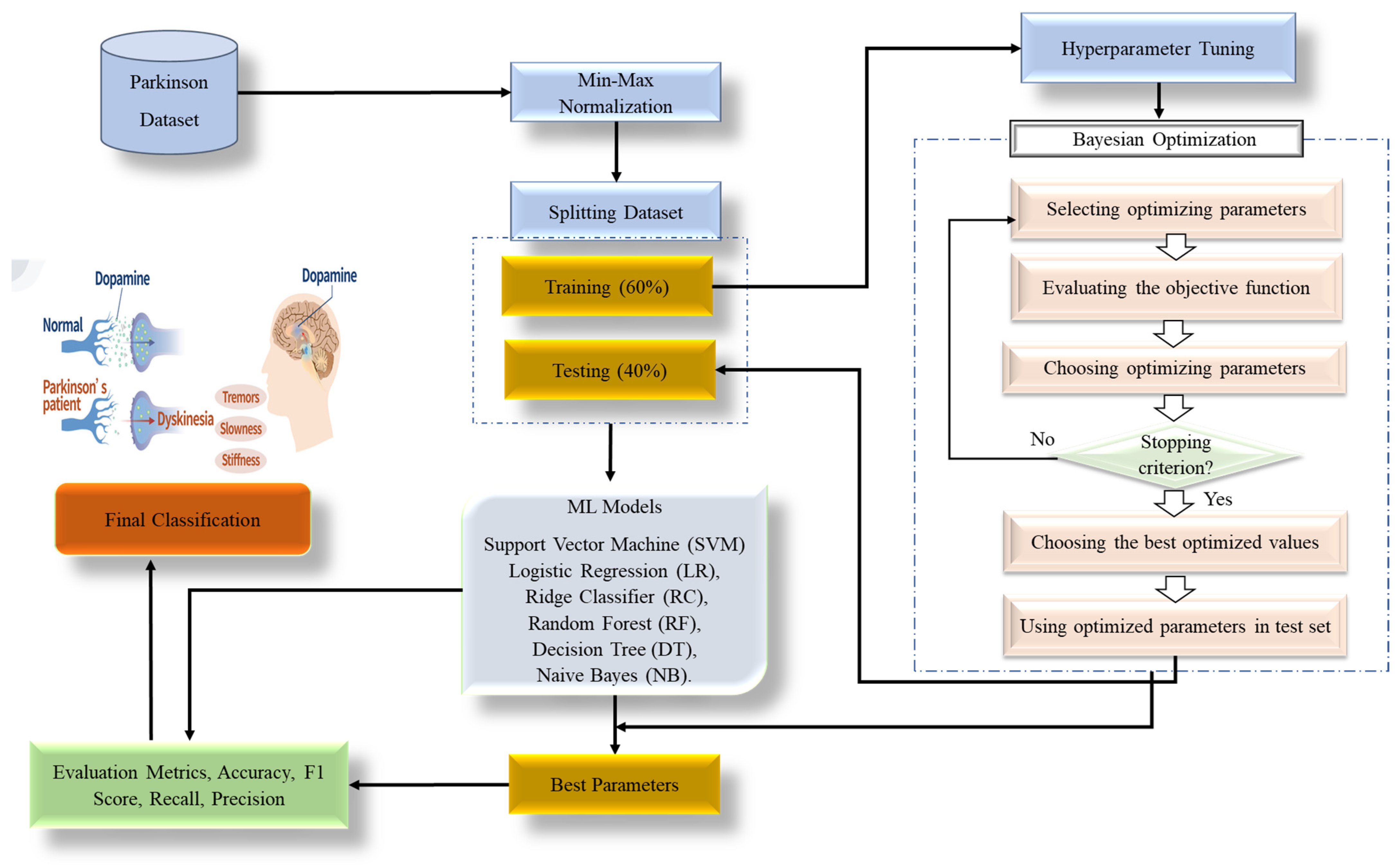
3. Materials and Methods
3.1. Min-Max Normalization
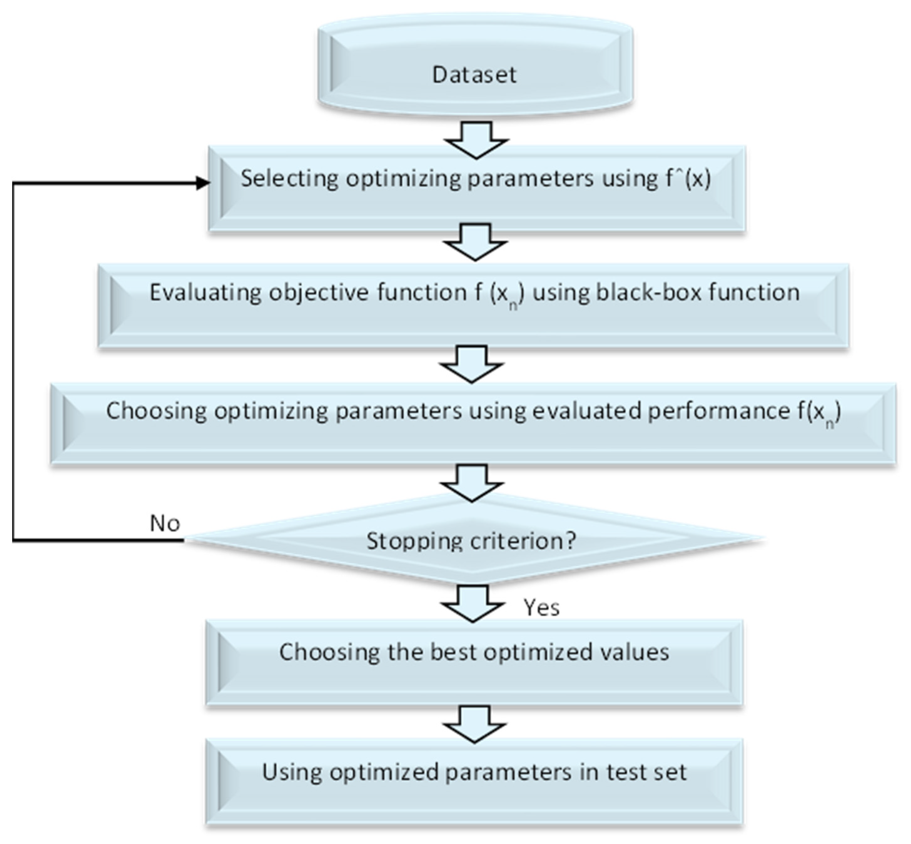
3.2. Bayesian Optimization
3.3. Machine Learning Models Using Bayesian Hyperparameter Optimization
| Algorithm 1. Bayesian Optimization-Support Vector Machine (BO-SVM) |
| Input: Dataset D, hyper-parameter space Θ, Target score function T(), max of evaluation nmax. Split randomly the D into N folds; one for train set and the other for test set. Build a model m on the train dataset using SVM approach. Choose a starting configuration θ0 Θ. Assess the original score y0 = T(θ0). Initialize S0 = {θ0, y0} While t < maximum number of iterations do For m = 1, …, mmax do Choose a new hyperparameter arrangement θm Θ by enhancing function Um Θm = max Um (, St), Analyze H in θm to get a new numerical score ym = T(θm). Strengthen the data {θm, ym}. Update the surrogate model. m = m + 1 End for End while Extract optimized hyperparameters. Build SVM model using these tuned hyperparameters from the test data set. Solve the optimization problem, evaluate the accuracy and save it in array. Output: Mean accuracy of classification. |
4. Experimental Results
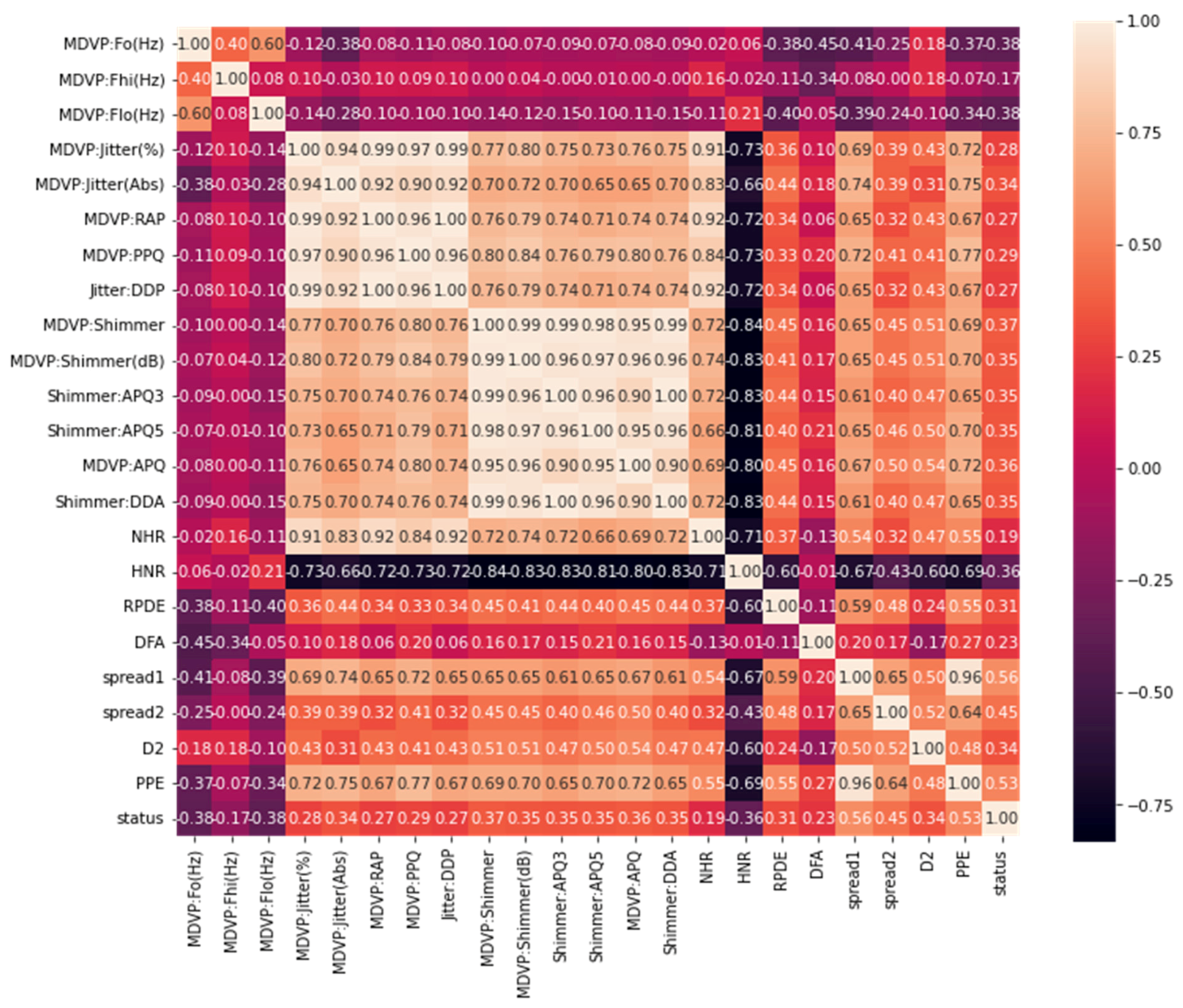
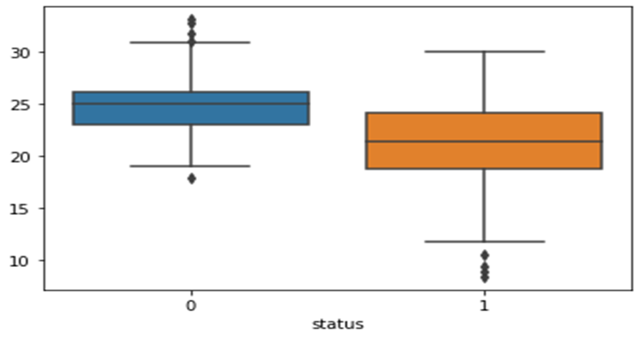
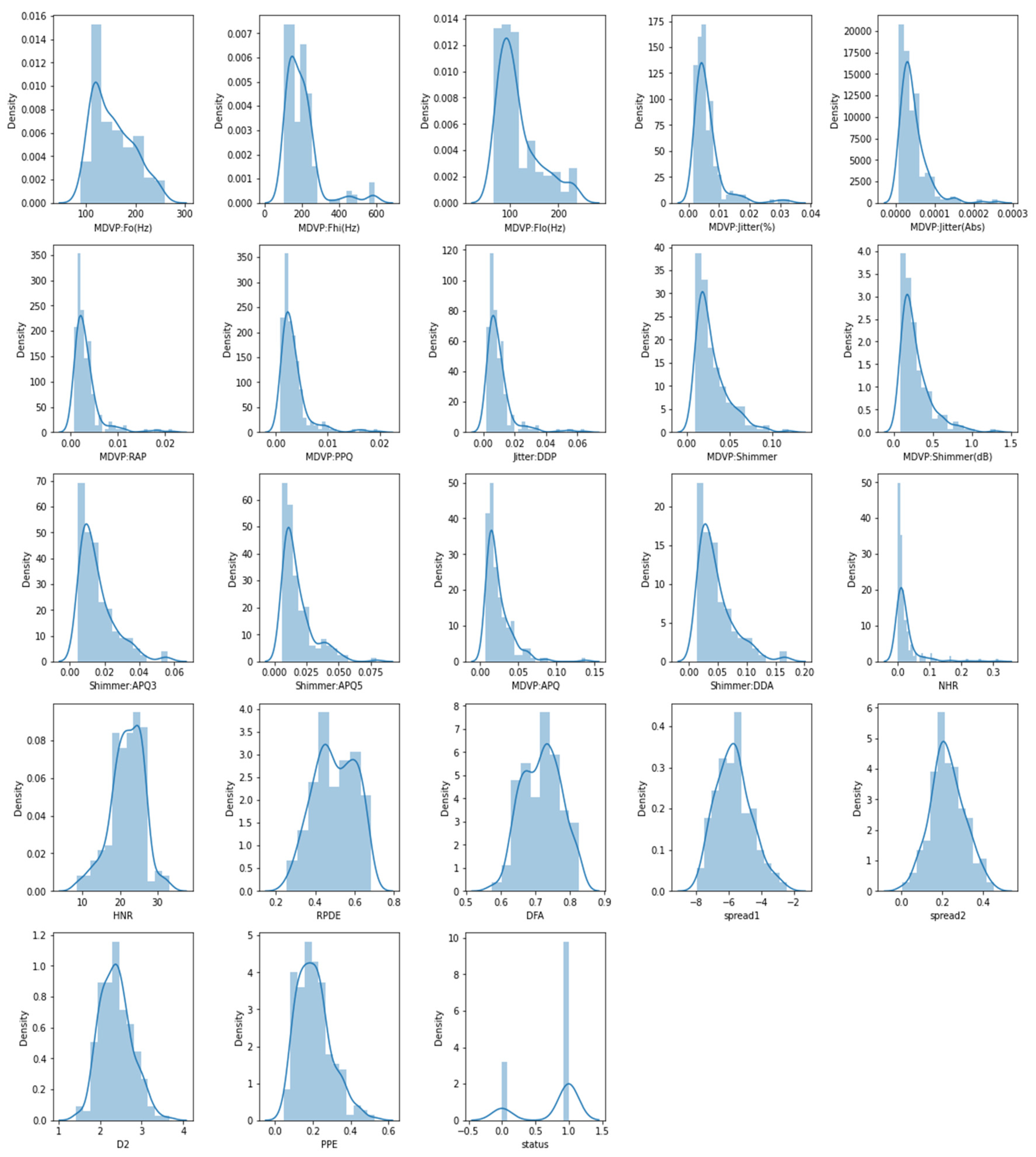
4.1. Dataset Description
4.2. Evaluation Metrics
- Random Forest (RF): The best number of estimators was 10, using the “gini” criterion.
- Ridge Classifier (RC): The best alpha was 0.4, with “copy_X” set to false, “fit_intercept” set to true, “normalize” set to false, and using the “lsqr” solver with a tolerance of 0.01.
- Decision Tree (DT): The best criterion was “entropy” and the best splitter was “random”.
- Naive Bayes (NB): The best alpha was 0.1 and the best value for “var_smoothing” was 0.00001.
- Logistic Regression (LR): The best penalty was “l2” and the best solver was “lbfgs”.
- Support Vector Machine (SVM): The best kernel was “rbf” and the best value for the regularization parameter (C) was 0.4.
4.3. Discussion
- Model-based approach: BO uses a probabilistic model to represent the relationship between the hyperparameters and the performance of the model. This allows BO to make informed decisions about which hyperparameters to try next based on the results of previous trials.
- Handling of noisy objectives: BO can handle noisy or stochastic objective functions, such as those that may be encountered in real-world machine learning applications.
- Incorporation of prior knowledge: BO allows for the incorporation of prior knowledge about the objective function through the use of a prior distribution over the hyperparameters.
- Efficient exploration–exploitation trade-off: BO balances exploration (trying new, potentially better hyperparameters) and exploitation (using the current best hyperparameters) in an efficient manner, allowing for faster convergence to the optimal hyperparameters.
5. Conclusions and Future Work
Author Contributions
Funding
Institutional Review Board Statement
Informed Consent Statement
Data Availability Statement
Conflicts of Interest
References
- Bloem, B.R.; Okun, M.S.; Klein, C. Parkinson’s Disease. Lancet 2021, 397, 2284–2303. [Google Scholar] [CrossRef] [PubMed]
- Mei, J.; Desrosiers, C.; Frasnelli, J. Machine Learning for the Diagnosis of Parkinson’s Disease: A Review of Literature. Front. Aging Neurosci. 2021, 13, 633752. [Google Scholar] [CrossRef] [PubMed]
- Landolfi, A.; Ricciardi, C.; Donisi, L.; Cesarelli, G.; Troisi, J.; Vitale, C.; Barone, P.; Amboni, M. Machine Learning Approaches in Parkinson’s Disease. Curr. Med. Chem. 2021, 28, 6548–6568. [Google Scholar] [CrossRef] [PubMed]
- Gao, C.; Sun, H.; Wang, T.; Tang, M.; Bohnen, N.I.; Müller, M.L.T.M.; Herman, T.; Giladi, N.; Kalinin, A.; Spino, C. Model-Based and Model-Free Machine Learning Techniques for Diagnostic Prediction and Classification of Clinical Outcomes in Parkinson’s Disease. Sci. Rep. 2018, 8, 7129. [Google Scholar] [CrossRef] [PubMed]
- Wang, W.; Lee, J.; Harrou, F.; Sun, Y. Early Detection of Parkinson’s Disease Using Deep Learning and Machine Learning. IEEE Access 2020, 8, 147635–147646. [Google Scholar] [CrossRef]
- Berg, D. Biomarkers for the Early Detection of Parkinson’s and Alzheimer’s Disease. Neurodegener. Dis. 2008, 5, 133–136. [Google Scholar] [CrossRef]
- Becker, G.; Müller, A.; Braune, S.; Büttner, T.; Benecke, R.; Greulich, W.; Klein, W.; Mark, G.; Rieke, J.; Thümler, R. Early Diagnosis of Parkinson’s Disease. J. Neurol. 2002, 249, iii40–iii48. [Google Scholar] [CrossRef]
- Sveinbjornsdottir, S. The Clinical Symptoms of Parkinson’s Disease. J. Neurochem. 2016, 139, 318–324. [Google Scholar] [CrossRef]
- DeMaagd, G.; Philip, A. Parkinson’s Disease and Its Management. Pharm. Ther. 2015, 40, 504–532. [Google Scholar]
- Shams, M.Y.; Elzeki, O.M.; Abouelmagd, L.M.; Hassanien, A.E.; Abd Elfattah, M.; Salem, H. HANA: A Healthy Artificial Nutrition Analysis Model during COVID-19 Pandemic. Comput. Biol. Med. 2021, 135, 104606. [Google Scholar] [CrossRef]
- Salem, H.; Shams, M.Y.; Elzeki, O.M.; Abd Elfattah, M.; Al-Amri, J.F.; Elnazer, S. Fine-Tuning Fuzzy KNN Classifier Based on Uncertainty Membership for the Medical Diagnosis of Diabetes. Appl. Sci. 2022, 12, 950. [Google Scholar] [CrossRef]
- Pham, H.; Do, T.; Chan, K.; Sen, G.; Han, A.; Lim, P.; Cheng, T.; Quang, N.; Nguyen, B.; Chua, M. Multimodal Detection of Parkinson Disease Based on Vocal and Improved Spiral Test. In Proceedings of the 2019 International Conference on System Science and Engineering (ICSSE), Dong Hoi, Vietnam, 20–21 July 2019; pp. 279–284. [Google Scholar]
- Pereira, C.R.; Pereira, D.R.; Rosa, G.H.; Albuquerque, V.H.C.; Weber, S.A.T.; Hook, C.; Papa, J.P. Handwritten Dynamics Assessment through Convolutional Neural Networks: An Application to Parkinson’s Disease Identification. Artif. Intell. Med. 2018, 87, 67–77. [Google Scholar] [CrossRef] [PubMed]
- Choi, H.; Ha, S.; Im, H.J.; Paek, S.H.; Lee, D.S. Refining Diagnosis of Parkinson’s Disease with Deep Learning-Based Interpretation of Dopamine Transporter Imaging. NeuroImage Clin. 2017, 16, 586–594. [Google Scholar] [CrossRef] [PubMed]
- Castillo-Barnes, D.; Ramírez, J.; Segovia, F.; Martínez-Murcia, F.J.; Salas-Gonzalez, D.; Górriz, J.M. Robust Ensemble Classification Methodology for I123-Ioflupane SPECT Images and Multiple Heterogeneous Biomarkers in the Diagnosis of Parkinson’s Disease. Front. Neuroinform. 2018, 12, 53. [Google Scholar] [CrossRef]
- Nuvoli, S.; Spanu, A.; Fravolini, M.L.; Bianconi, F.; Cascianelli, S.; Madeddu, G.; Palumbo, B. [(123)I] Metaiodobenzylguanidine (MIBG) Cardiac Scintigraphy and Automated Classification Techniques in Parkinsonian Disorders. Mol. Imaging Biol. 2020, 22, 703–710. [Google Scholar] [CrossRef]
- Adeli, E.; Shi, F.; An, L.; Wee, C.-Y.; Wu, G.; Wang, T.; Shen, D. Joint Feature-Sample Selection and Robust Diagnosis of Parkinson’s Disease from MRI Data. NeuroImage 2016, 141, 206–219. [Google Scholar] [CrossRef]
- Nunes, A.; Silva, G.; Duque, C.; Januário, C.; Santana, I.; Ambrósio, A.F.; Castelo-Branco, M.; Bernardes, R. Retinal Texture Biomarkers May Help to Discriminate between Alzheimer’s, Parkinson’s, and Healthy Controls. PLoS ONE 2019, 14, e0218826. [Google Scholar] [CrossRef] [PubMed]
- Das, R. A Comparison of Multiple Classification Methods for Diagnosis of Parkinson Disease. Expert Syst. Appl. 2010, 37, 1568–1572. [Google Scholar] [CrossRef]
- Åström, F.; Koker, R. A Parallel Neural Network Approach to Prediction of Parkinson’s Disease. Expert Syst. Appl. 2011, 38, 12470–12474. [Google Scholar] [CrossRef]
- Bhattacharya, I.; Bhatia, M.P.S. SVM Classification to Distinguish Parkinson Disease Patients. In Proceedings of the 1st Amrita ACM-W Celebration on Women in Computing in India, New York, NY, USA, 16 September 2010; pp. 1–6. [Google Scholar]
- Chen, H.-L.; Huang, C.-C.; Yu, X.-G.; Xu, X.; Sun, X.; Wang, G.; Wang, S.-J. An Efficient Diagnosis System for Detection of Parkinson’s Disease Using Fuzzy k-Nearest Neighbor Approach. Expert Syst. Appl. 2013, 40, 263–271. [Google Scholar] [CrossRef]
- Li, D.-C.; Liu, C.-W.; Hu, S.C. A Fuzzy-Based Data Transformation for Feature Extraction to Increase Classification Performance with Small Medical Data Sets. Artif. Intell. Med. 2011, 52, 45–52. [Google Scholar] [CrossRef] [PubMed]
- Eskidere, Ö.; Ertaş, F.; Hanilçi, C. A Comparison of Regression Methods for Remote Tracking of Parkinson’s Disease Progression. Expert Syst. Appl. 2012, 39, 5523–5528. [Google Scholar] [CrossRef]
- Nilashi, M.; Ibrahim, O.; Ahani, A. Accuracy Improvement for Predicting Parkinson’s Disease Progression. Sci. Pep. 2016, 6, 34181. [Google Scholar] [CrossRef] [PubMed]
- Peterek, T.; Dohnálek, P.; Gajdoš, P.; Šmondrk, M. Performance Evaluation of Random Forest Regression Model in Tracking Parkinson’s Disease Progress. In Proceedings of the 13th International Conference on Hybrid Intelligent Systems (HIS 2013), Gammarth, Tunisia, 4–6 December 2013; pp. 83–87. [Google Scholar]
- Karimi-Rouzbahani, H.; Daliri, M. Diagnosis of Parkinson’s Disease in Human Using Voice Signals. Basic Clin. Neurosci. 2011, 2, 12. [Google Scholar]
- Ma, A.; Lau, K.K.; Thyagarajan, D. Voice Changes in Parkinson’s Disease: What Are They Telling Us? J. Clin. Neurosci. Off. J. Neurosurg. Soc. Australas. 2020, 72, 1–7. [Google Scholar] [CrossRef]
- Mudali, D.; Teune, L.K.; Renken, R.J.; Leenders, K.L.; Roerdink, J.B.T.M. Classification of Parkinsonian Syndromes from FDG-PET Brain Data Using Decision Trees with SSM/PCA Features. Comput. Math. Methods Med. 2015, 2015, 136921. [Google Scholar] [CrossRef]
- Tsanas, A.; Little, M.A.; McSharry, P.E.; Ramig, L.O. Enhanced Classical Dysphonia Measures and Sparse Regression for Telemonitoring of Parkinson’s Disease Progression. In Proceedings of the 2010 IEEE International Conference on Acoustics, Speech and Signal Processing, Dallas, TX, USA, 14–19 March 2010; pp. 594–597. [Google Scholar]
- Shahid, A.H.; Singh, M.P. A Deep Learning Approach for Prediction of Parkinson’s Disease Progression. Biomed. Eng. Lett. 2020, 10, 227–239. [Google Scholar] [CrossRef]
- Fernandes, C.; Fonseca, L.; Ferreira, F.; Gago, M.; Costa, L.; Sousa, N.; Ferreira, C.; Gama, J.; Erlhagen, W.; Bicho, E. Artificial Neural Networks Classification of Patients with Parkinsonism Based on Gait. In Proceedings of the 2018 IEEE International Conference on Bioinformatics and Biomedicine (BIBM), New York, NY, USA, 3–6 December 2018. [Google Scholar]
- Ghassemi, N.H.; Marxreiter, F.; Pasluosta, C.F.; Kugler, P.; Schlachetzki, J.; Schramm, A.; Eskofier, B.M.; Klucken, J. Combined Accelerometer and EMG Analysis to Differentiate Essential Tremor from Parkinson’s Disease. Annu. Int. Conf. IEEE Eng. Med. Biol. Soc. 2016, 2016, 672–675. [Google Scholar] [CrossRef]
- Abiyev, R.H.; Abizade, S. Diagnosing Parkinson’s Diseases Using Fuzzy Neural System. Comput. Math. Methods Med. 2016, 2016, 1267919. [Google Scholar] [CrossRef]
- Vlachostergiou, A.; Tagaris, A.; Stafylopatis, A.; Kollias, S. Multi-Task Learning for Predicting Parkinson’s Disease Based on Medical Imaging Information. In Proceedings of the 2018 25th IEEE International Conference on Image Processing (ICIP), Athens, Greece, 7–10 October 2018; pp. 2052–2056. [Google Scholar]
- Liu, L.; Wang, Q.; Adeli, E.; Zhang, L.; Zhang, H.; Shen, D. Feature Selection Based on Iterative Canonical Correlation Analysis for Automatic Diagnosis of Parkinson’s Disease. In Proceedings of the Medical Image Computing and Computer-Assisted Intervention–MICCAI 2016: 19th International Conference, Athens, Greece, October 17–21 2016; Springer: Berlin/Heidelberg, Germany, 2016; pp. 1–8. [Google Scholar]
- Drotár, P.; Mekyska, J.; Rektorová, I.; Masarová, L.; Smékal, Z.; Faundez-Zanuy, M. Analysis of In-Air Movement in Handwriting: A Novel Marker for Parkinson’s Disease. Comput. Methods Programs Biomed. 2014, 117, 405–411. [Google Scholar] [CrossRef]
- Eesa, A.S.; Arabo, W.K. A Normalization Methods for Backpropagation: A Comparative Study. Sci. J. Univ. Zakho 2017, 5, 319–323. [Google Scholar] [CrossRef]
- Victoria, A.H.; Maragatham, G. Automatic Tuning of Hyperparameters Using Bayesian Optimization. Evol. Syst. 2021, 12, 217–223. [Google Scholar] [CrossRef]
- Cho, H.; Kim, Y.; Lee, E.; Choi, D.; Lee, Y.; Rhee, W. Basic Enhancement Strategies When Using Bayesian Optimization for Hyperparameter Tuning of Deep Neural Networks. IEEE Access 2020, 8, 52588–52608. [Google Scholar] [CrossRef]
- Hussain, L.; Malibari, A.A.; Alzahrani, J.S.; Alamgeer, M.; Obayya, M.; Al-Wesabi, F.N.; Mohsen, H.; Hamza, M.A. Bayesian Dynamic Profiling and Optimization of Important Ranked Energy from Gray Level Co-Occurrence (GLCM) Features for Empirical Analysis of Brain MRI. Sci. Rep. 2022, 12, 15389. [Google Scholar] [CrossRef] [PubMed]
- Eltahir, M.M.; Hussain, L.; Malibari, A.A.; Nour, M.K.; Obayya, M.; Mohsen, H.; Yousif, A.; Ahmed Hamza, M. A Bayesian Dynamic Inference Approach Based on Extracted Gray Level Co-Occurrence (GLCM) Features for the Dynamical Analysis of Congestive Heart Failure. Appl. Sci. 2022, 12, 6350. [Google Scholar] [CrossRef]
- Wu, J.; Chen, X.-Y.; Zhang, H.; Xiong, L.-D.; Lei, H.; Deng, S.-H. Hyperparameter Optimization for Machine Learning Models Based on Bayesian Optimization. J. Electron. Sci. Technol. 2019, 17, 26–40. [Google Scholar]
- Kramer, O.; Ciaurri, D.E.; Koziel, S. Derivative-Free Optimization. In Computational Optimization, Methods and Algorithms; Springer: Berlin/Heidelberg, Germany, 2011; pp. 61–83. [Google Scholar]
- UCI Machine Learning Repository. Parkinsons Data Set. 2007. Available online: http://archive.ics.uci.edu/ml/datasets/Parkinsons (accessed on 30 December 2022).
- Jakkula, V. Tutorial on Support Vector Machine (Svm). Sch. EECS Wash. State Univ. 2006, 37, 3. [Google Scholar]
- Cutler, A.; Cutler, D.R.; Stevens, J.R. Random Forests. In Ensemble Machine Learning; Springer: Berlin/Heidelberg, Germany, 2012; pp. 157–175. [Google Scholar]
- Nick, T.G.; Campbell, K.M. Logistic Regression. Top. Biostat. 2007, 404, 273–301. [Google Scholar]
- Zhang, H. The Optimality of Naive Bayes. Aa 2004, 1, 1–6. [Google Scholar]
- Xingyu, M.A.; Bolei, M.A.; Qi, F. Logistic Regression and Ridge Classifier. 2022. Available online: https://www.cis.uni-muenchen.de/~stef/seminare/klassifikation_2021/referate/LogisticRegressionRidgeClassifier.pdf (accessed on 28 January 2023).
- Kotsiantis, S.B. Decision Trees: A Recent Overview. Artif. Intell. Rev. 2013, 39, 261–283. [Google Scholar] [CrossRef]
- Najwa Mohd Rizal, N.; Hayder, G.; Mnzool, M.; Elnaim, B.M.; Mohammed, A.O.Y.; Khayyat, M.M. Comparison between Regression Models, Support Vector Machine (SVM), and Artificial Neural Network (ANN) in River Water Quality Prediction. Processes 2022, 10, 1652. [Google Scholar] [CrossRef]
- Alabdulkreem, E.; Alzahrani, J.S.; Eltahir, M.M.; Mohamed, A.; Hamza, M.A.; Motwakel, A.; Eldesouki, M.I.; Rizwanullah, M. Cuckoo Optimized Convolution Support Vector Machine for Big Health Data Processing. Comput. Mater. Contin. 2022, 73, 3039–3055. [Google Scholar] [CrossRef]
- Al Duhayyim, M.; Mohamed, H.G.; Alotaibi, S.S.; Mahgoub, H.; Mohamed, A.; Motwakel, A.; Zamani, A.S.; Eldesouki, M. Hyperparameter Tuned Deep Learning Enabled Cyberbullying Classification in Social Media. Comput. Mater. Contin. 2022, 73, 5011–5024. [Google Scholar] [CrossRef]
- Lauraitis, A.; Maskeliūnas, R.; Damaševičius, R.; Krilavičius, T. Detection of Speech Impairments Using Cepstrum, Auditory Spectrogram and Wavelet Time Scattering Domain Features. IEEE Access 2020, 8, 96162–96172. [Google Scholar] [CrossRef]
- Li, D.-C.; Hu, S.C.; Lin, L.-S.; Yeh, C.-W. Detecting Representative Data and Generating Synthetic Samples to Improve Learning Accuracy with Imbalanced Data Sets. PLoS ONE 2017, 12, e0181853. [Google Scholar] [CrossRef] [PubMed]
- Sajal, M.; Rahman, S.; Ehsan, M.; Vaidyanathan, R.; Wang, S.; Aziz, T.; Mamun, K.A.A. Telemonitoring Parkinson’s Disease Using Machine Learning by Combining Tremor and Voice Analysis. Brain Inform. 2020, 7, 12. [Google Scholar] [CrossRef] [PubMed]
- Haritha, K.; Judy, M.V.; Papageorgiou, K.; Georgiannis, V.C.; Papageorgiou, E. Distributed Fuzzy Cognitive Maps for Feature Selection in Big Data Classification. Algorithms 2022, 15, 383. [Google Scholar] [CrossRef]
- Abayomi-Alli, O.O.; Damaševičius, R.; Maskeliūnas, R.; Abayomi-Alli, A. BiLSTM with Data Augmentation Using Interpolation Methods to Improve Early Detection of Parkinson Disease. In Proceedings of the 2020 15th Conference on Computer Science and Information Systems (FedCSIS), Sofia, Bulgaria, 6–9 September 2020; pp. 371–380. [Google Scholar]
- Fang, L.; Liang, X. A Novel Method Based on Nonlinear Binary Grasshopper Whale Optimization Algorithm for Feature Selection. J. Bionic Eng. 2022, 20, 237–252. [Google Scholar] [CrossRef]


| Ref | Objective | Data Source & Sample Size | Techniques | Outcome | Benefits | Limitations |
|---|---|---|---|---|---|---|
| [29] | Diagnosis and classification of PD from HC | Private dataset from 38 individuals 20 PD and 18 Health Control (HC) | C4.5 Decision Tree the extracted features using PCA | LOOCV = 63.20% | The fundamental issue in clinical practice is not so much distinguishing individuals with Parkinsonian disorders from healthy controls | A huge amount of patient data must be collected at various stages of illness development |
| [30] | Diagnosis and classification of PD from MCI | Private dataset 42 subjects from PD patients | Feature selection based on LASSO | MAE = 8.38 | Because the new probability distributions span a wider normalized range, log-transformed measures outperformed their linear counterparts | Depending on linear regression which underperforms with non-linear decision boundaries |
| [31] | Diagnosis and classification of PD from HC | Private dataset from 10 medical centers of 10 PD patients | Deep Learning | R2 = 0.956 | Using DL help in identifying more insights in the dataset | Small datasets affect model and robustness increase the training time |
| [32] | Diagnosis and classification of PD from MCI | Gait data from 15 IPD, 15 VaP, and 15 healthy participants were collected using wearable sensors placed on both feet | MLP DBN | ACC = 94.50% ACC = 93.50% | They utilized a classification approach based on two different classifiers MLP and DBN with a better performance such that the problem is the differentiation between VaP and IPD | In balance, dataset affects model generalization ability |
| [33] | Classification of patients with essential tremor (ET) from tremor-dominant Parkinson disease (PD) | 13 PD patients (tremor dominant forms) and 11 ET patients | SVM | ACC of SVM with RBF = 83.00% | Classification of patients with essential tremor (ET) from tremor-dominant Parkinson disease (PD) | 13 PD patients (tremor dominant forms) and 11 ET patients |
| [34] | Classification of PD from HC | UCI data include voice measurements of 31 people | DNN SVM And Fuzzy neural system | ACC = 81.03% | Use hybrid model between NN and fuzzy system | Very small dataset with trained samples |
| [35] | Classification of PD from HC | 55 patients with Parkinson’s and 23 subjects with Parkinson’s related syndromes | (DNNs) with shared hidden layers. | ACC = 92.00% | Predicting Parkinson’s illness with multitask learning | Data on disease duration and treatment (i.e., treatment duration and dose) |
| [36] | Classification between PD and normal control | (56 PD, and 56 Normal Control) | Linear classifier | ACC = 89.00% F-Measure = 87.00% | Using iterative canonical correlation analysis for feature selection | The model needs to be tested with different train test splits |
| [37] | Classification between PD and HC | Handwriting of a sentence in 37 PD patients | SVM | ACC = −84.00% | Choosing optimal features based on sequential forward feature selection (SFFS) | Handwriting may overlap with other diseases |
| Column Name | Description |
|---|---|
| Name/ASCII | Patient’s name/Record Num |
| MDVP-Fo (Hz) | Vocal fundamental (mean frequency) |
| MDVP Fhi (Hz) | Vocal fundamental (Max frequency) |
| MDVP Flo (Hz) | Vocal fundamental (Min frequency) |
| MDVP jitter (%) | Several measurements differ in fundamental frequency (i.e., RAP, MDVP, APQ, etc.) |
| MDVP Fhi (Hz) | Several measurements differ in amplitude (i.e., APQ5, MDVP: APQ, etc.) |
| NHR, HNR | The ratio of noise with regard to total components in voice |
| RPDE, D2 | Nonlinear complexity measurements |
| DFA | Fractal scaling exponent |
| PPE, spread1, spread2 | Three nonlinear methods for calculating fundamental frequency variation |
| Count | Mean | Std | Min | 50% | Max | |
|---|---|---|---|---|---|---|
| MDVP:Fo(Hz) | 195.0 | 154.2286 | 41.390065 | 88.33300 | 148.7900 | 260.1050 |
| MDVP:Fhi(Hz) | 195.0 | 197.1049 | 91.491548 | 102.1450 | 175.8290 | 592.0300 |
| MDVP:Flo(Hz) | 195.0 | 116.3246 | 43.521413 | 65.47600 | 104.3150 | 239.1700 |
| MDVP:Jitter(%) | 195.0 | 0.006220 | 0.004848 | 0.001680 | 0.004940 | 0.033160 |
| MDVP:Jitter(Abs) | 195.0 | 0.000044 | 0.000035 | 0.000007 | 0.000030 | 0.000260 |
| MDVP:RAP | 195.0 | 0.003306 | 0.002968 | 0.000680 | 0.002500 | 0.021440 |
| MDVP:PPQ | 195.0 | 0.003446 | 0.002759 | 0.000920 | 0.002690 | 0.019580 |
| Jitter:DDP | 195.0 | 0.009920 | 0.008903 | 0.002040 | 0.007490 | 0.064330 |
| MDVP:Shimmer | 195.0 | 0.029709 | 0.018857 | 0.009540 | 0.022970 | 0.119080 |
| MDVP:Shimmer(dB) | 195.0 | 0.282251 | 0.194877 | 0.085000 | 0.221000 | 1.302000 |
| Shimmer:APQ3 | 195.0 | 0.015664 | 0.010153 | 0.004550 | 0.012790 | 0.056470 |
| Shimmer:APQ5 | 195.0 | 0.017878 | 0.012024 | 0.005700 | 0.013470 | 0.079400 |
| MDVP:APQ | 195.0 | 0.024081 | 0.016947 | 0.007190 | 0.018260 | 0.137780 |
| Shimmer:DDA | 195.0 | 0.046993 | 0.030459 | 0.013640 | 0.038360 | 0.169420 |
| NHR | 195.0 | 0.024847 | 0.040418 | 0.000650 | 0.011660 | 0.314820 |
| HNR | 195.0 | 21.88597 | 4.425764 | 8.441000 | 22.085000 | 33.04700 |
| RPDE | 195.0 | 0.498536 | 0.103942 | 0.256570 | 0.495954 | 0.685151 |
| DFA | 195.0 | 0.718099 | 0.055336 | 0.574282 | 0.722254 | 0.825288 |
| spread1 | 195.0 | −5.684397 | 1.090208 | −7.964984 | −5.720868 | −2.434031 |
| spread2 | 195.0 | 0.226510 | 0.083406 | 0.006274 | 0.218885 | 0.450493 |
| D2 | 195.0 | 2.381826 | 0.382799 | 1.423287 | 2.361532 | 3.671155 |
| PPE | 195.0 | 0.206552 | 0.090119 | 0.044539 | 0.194052 | 0.527367 |
| Status | 195.0 | 0.753846 | 0.431878 | 0.000000 | 1.000000 | 1.000000 |
| Models | Best Hyperparameters |
|---|---|
| RF | N_estimators = 10, criterion = gini. |
| RC | Alpha = 0.4, copy_X = false, fit_intercept = true, normalize = false, solver = lsqr, tol = 0.01. |
| DT | Criterion = entropy, splitter = random. |
| NB | Alpha = 0.1, var_smoothing = 0.00001. |
| LR | Penalty = l2, solver = lbfgs. |
| SVM | Kernel = rbf, regularization parameter (C) = 0.4. |
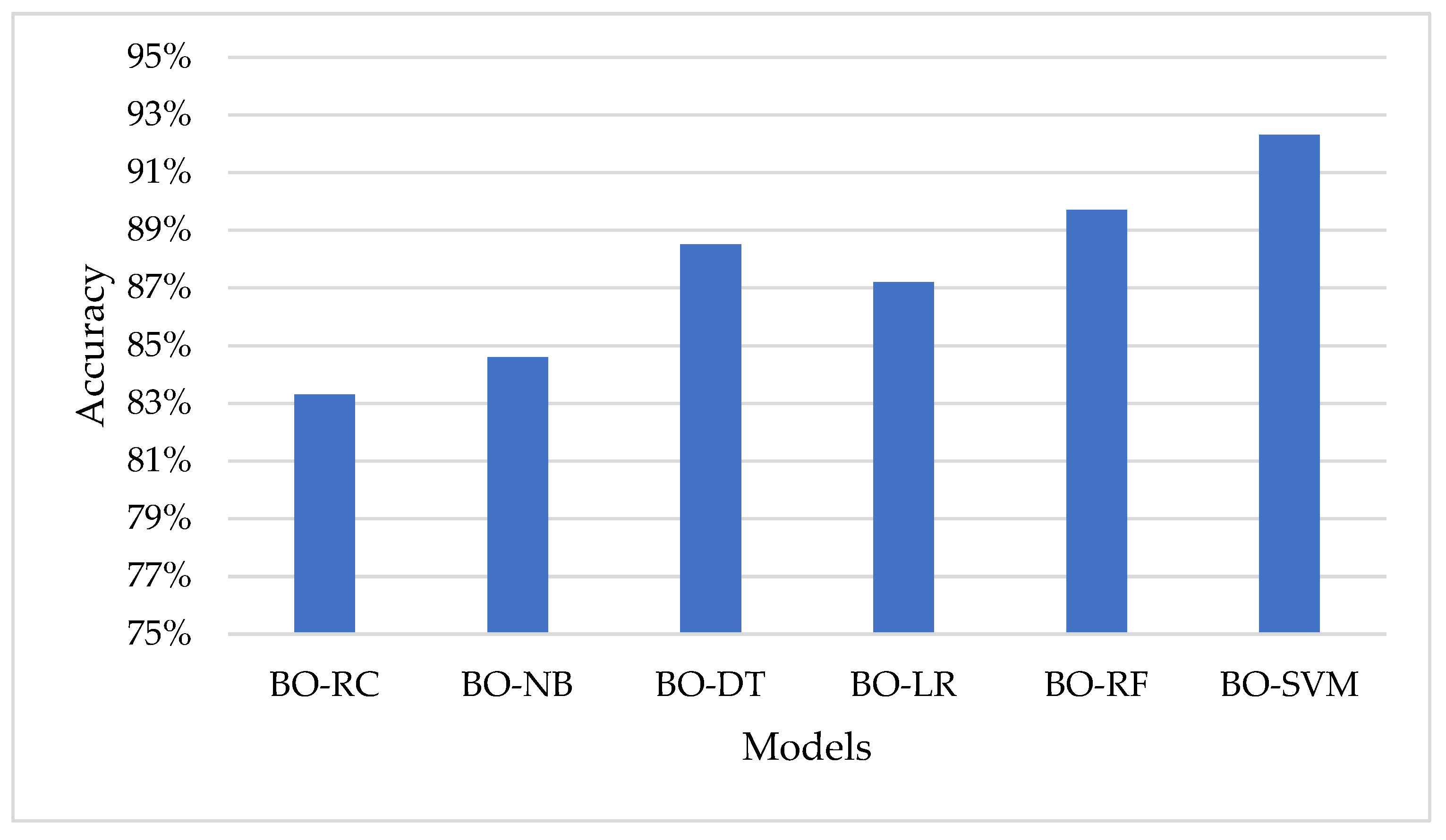
| Models | Accuracy | F1 Score | Recall | Precision |
|---|---|---|---|---|
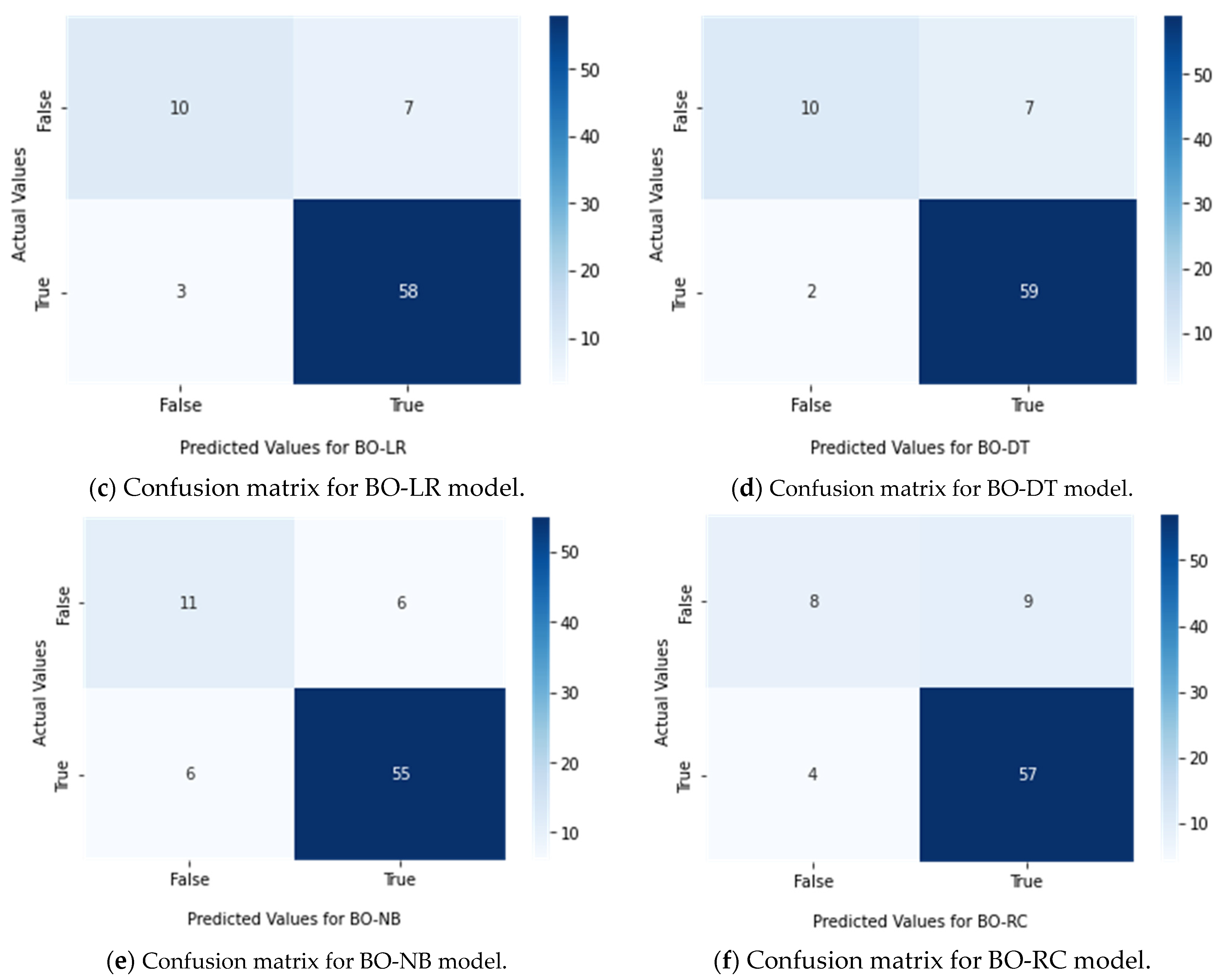
| BO-RC | 83.3% | 82.2% | 83.3% | 82.0% |
| BO-NB | 84.6% | 84.4% | 86.6% | 84.5% |
| BO-DT | 88.5% | 87.7% | 88.5% | 88.0% |
| BO-LR | 87.2% | 86.5% | 87.2% | 86.5% |
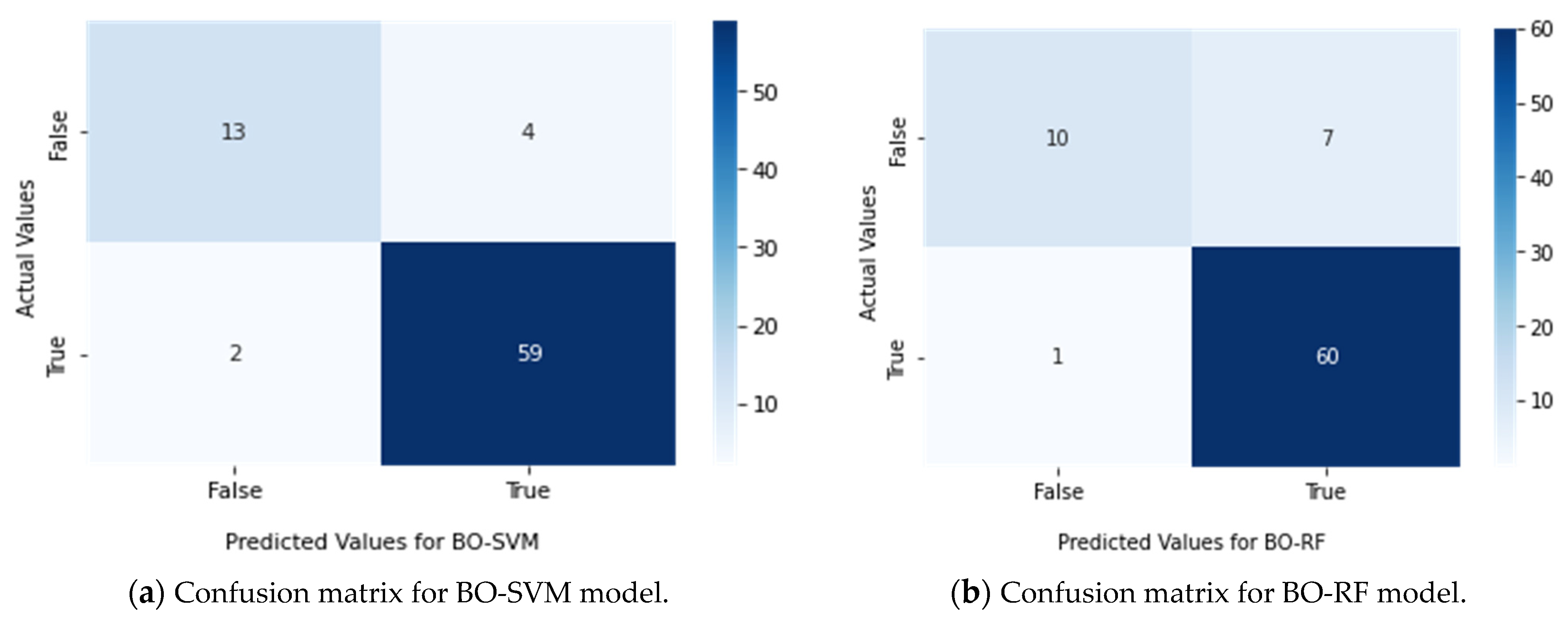
| BO-RF | 89.7% | 88.9% | 89.7% | 89.8% |
| BO-SVM | 92.3% | 92.1% | 92.3% | 92.1% |
| Models | Accuracy |
|---|---|
| RC | 80.9% |
| NB | 82.1% |
| DT | 85.7% |
| LR | 85.3% |
| RF | 87.2% |
| SVM | 89.6% |
Disclaimer/Publisher’s Note: The statements, opinions and data contained in all publications are solely those of the individual author(s) and contributor(s) and not of MDPI and/or the editor(s). MDPI and/or the editor(s) disclaim responsibility for any injury to people or property resulting from any ideas, methods, instructions or products referred to in the content. |
© 2023 by the authors. Licensee MDPI, Basel, Switzerland. This article is an open access article distributed under the terms and conditions of the Creative Commons Attribution (CC BY) license (https://creativecommons.org/licenses/by/4.0/).
Share and Cite
Elshewey, A.M.; Shams, M.Y.; El-Rashidy, N.; Elhady, A.M.; Shohieb, S.M.; Tarek, Z. Bayesian Optimization with Support Vector Machine Model for Parkinson Disease Classification. Sensors 2023, 23, 2085. https://doi.org/10.3390/s23042085
Elshewey AM, Shams MY, El-Rashidy N, Elhady AM, Shohieb SM, Tarek Z. Bayesian Optimization with Support Vector Machine Model for Parkinson Disease Classification. Sensors. 2023; 23(4):2085. https://doi.org/10.3390/s23042085
Chicago/Turabian StyleElshewey, Ahmed M., Mahmoud Y. Shams, Nora El-Rashidy, Abdelghafar M. Elhady, Samaa M. Shohieb, and Zahraa Tarek. 2023. "Bayesian Optimization with Support Vector Machine Model for Parkinson Disease Classification" Sensors 23, no. 4: 2085. https://doi.org/10.3390/s23042085
APA StyleElshewey, A. M., Shams, M. Y., El-Rashidy, N., Elhady, A. M., Shohieb, S. M., & Tarek, Z. (2023). Bayesian Optimization with Support Vector Machine Model for Parkinson Disease Classification. Sensors, 23(4), 2085. https://doi.org/10.3390/s23042085