


An Elastic Self-Adjusting Technique for Rare-Class Synthetic Oversampling Based on Cluster Distortion Minimization in Data Stream

Abstract
:1. Introduction
- It chooses the most valuable previous rare-class instances based on their quality to preserve the coherence of the current data chunk.
- For this task, it utilized the evaluation of Cluster Distortion measurement rather than merely using the mean of values as ADWIN.
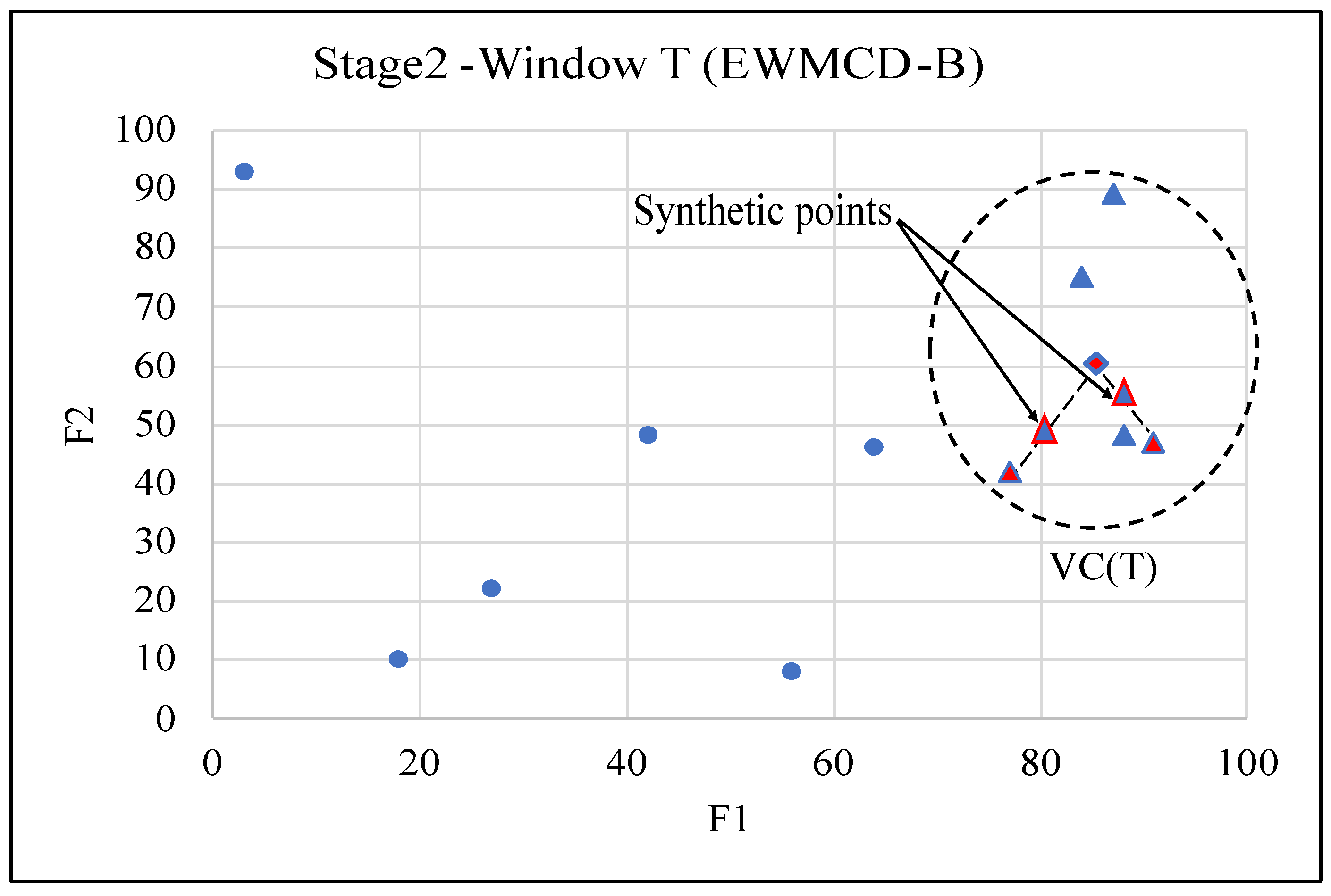
- It generates synthetic data points from the real selected candidates inspired by SMOTE (Synthetic Minority Oversampling Technique) to avoid repeating the same old instances; in addition, many of these synthetic points will be closer to the current chuck.
- The implementation utilized the two proposed models to significantly enhance the effectiveness of the adaptive classifiers for the EEG signals. It provides a more independent model for seizure detection with signals generated from wearable sensors of epileptic patients.
2. Literature Review
2.1. Classification of Imbalance Data Stream
2.2. Synthetic Rare-Class Oversampling
2.3. Cluster Distortion Minimization
2.4. Related Works
3. Methodology
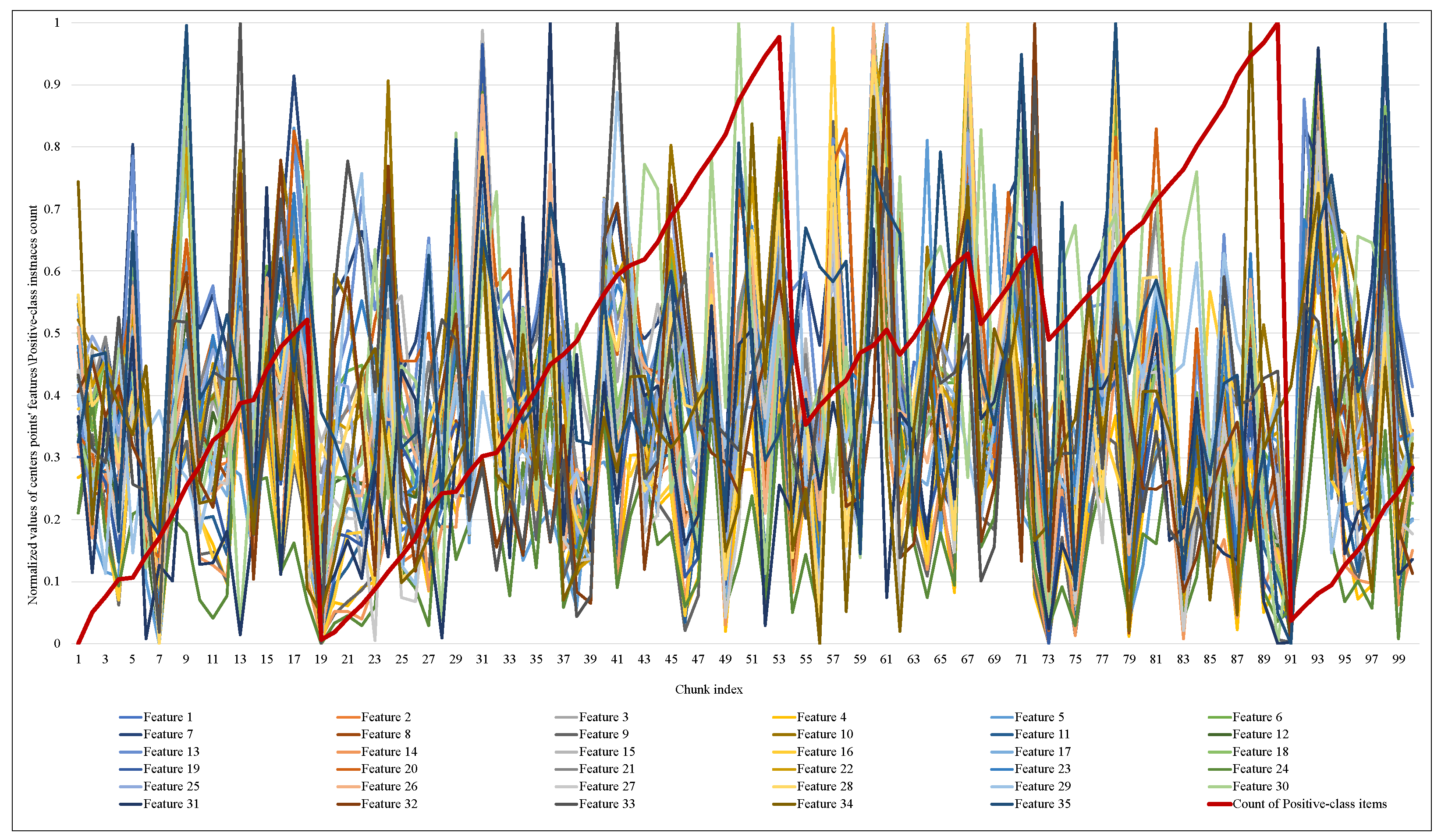
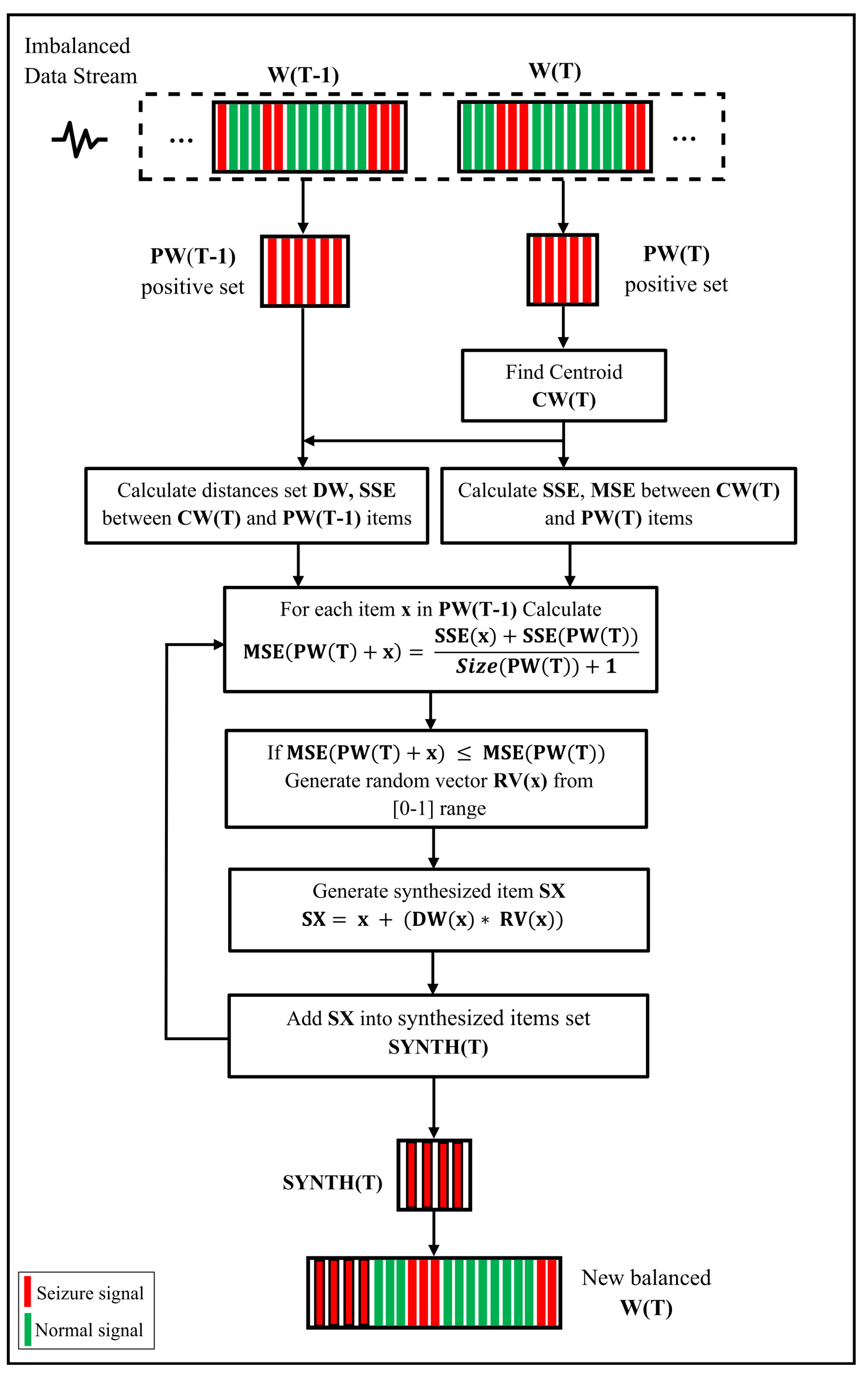
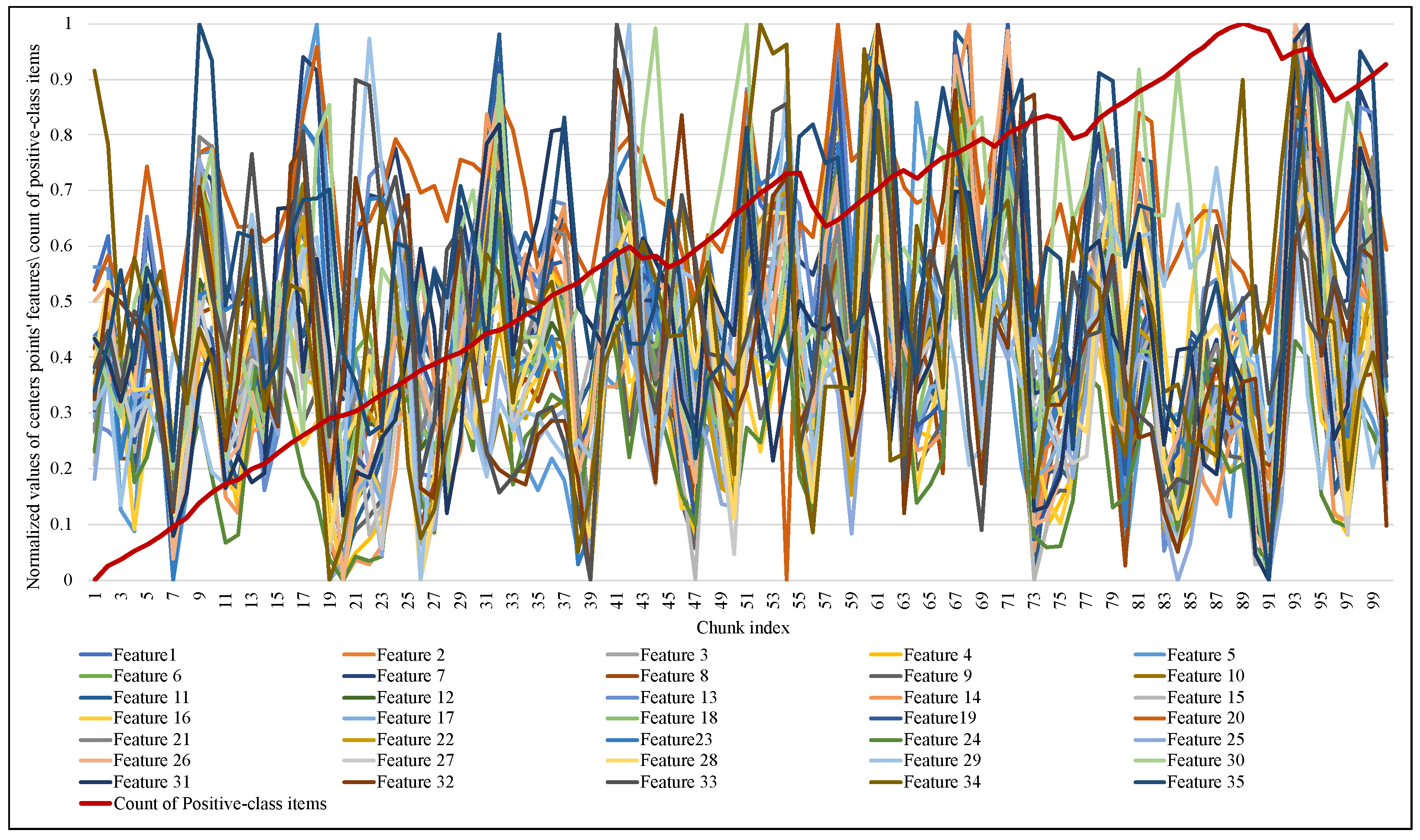
3.1. Selecting Elementary MCD Itemset
| Algorithm 1 Algorithm of the first stage of EWMCD-A. |
| Input: Stream Chunk W(T) and W(T − 1) |
|
| Output: MCD itemset, CW(T) |
| Algorithm 2 Algorithm of the first stage of EWMCD-B. |
| Input: Stream Chunk W(T) and W(T − 1) |
|
| Output: MCD itemset, CW(T) |
3.2. Generating Synthetic MCD Itemset
| Algorithm 3 Algorithm of the second stage of EWMCD-A and EWMCD-B. |
| Input: Stream Chunk W(T), MCD itemset, and CW(T) |
|
| Output: Adapted Window (T) |
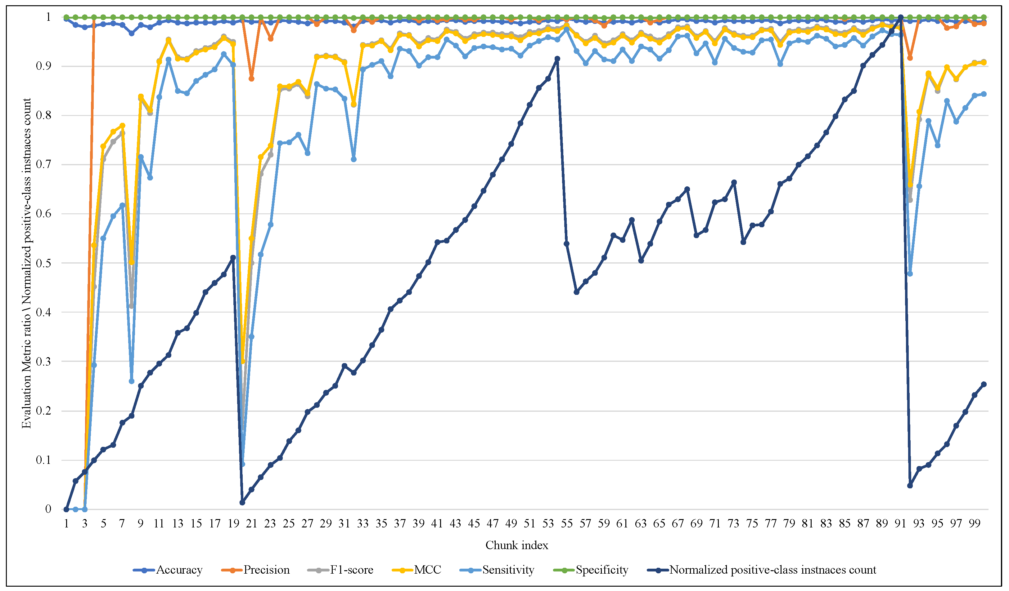
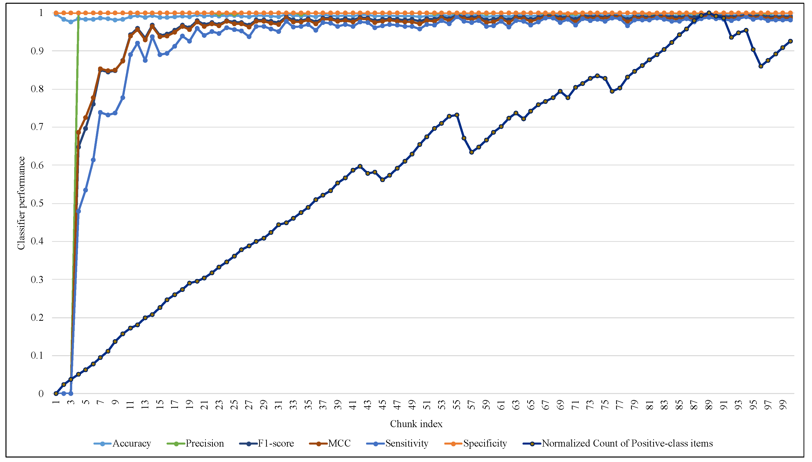
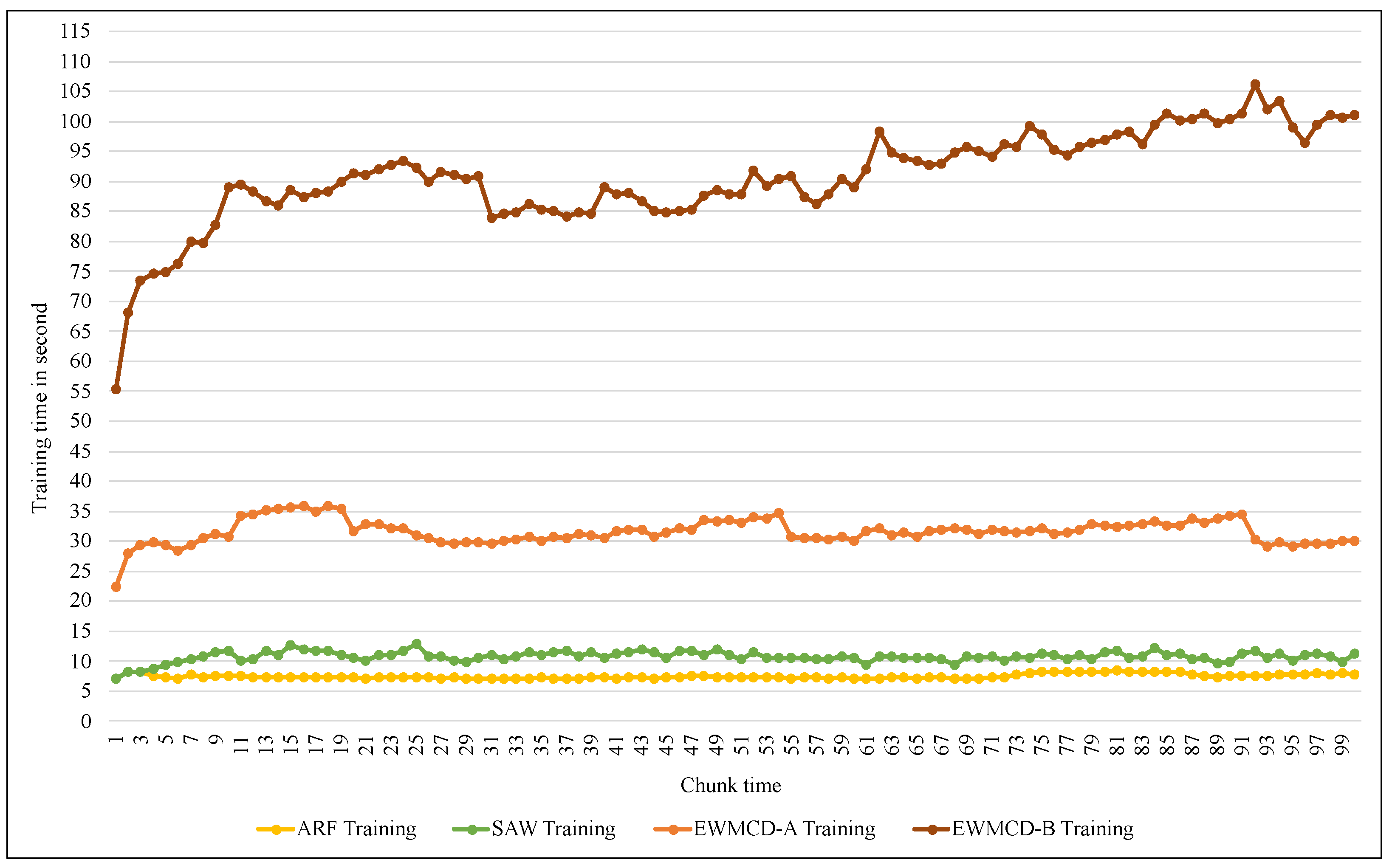
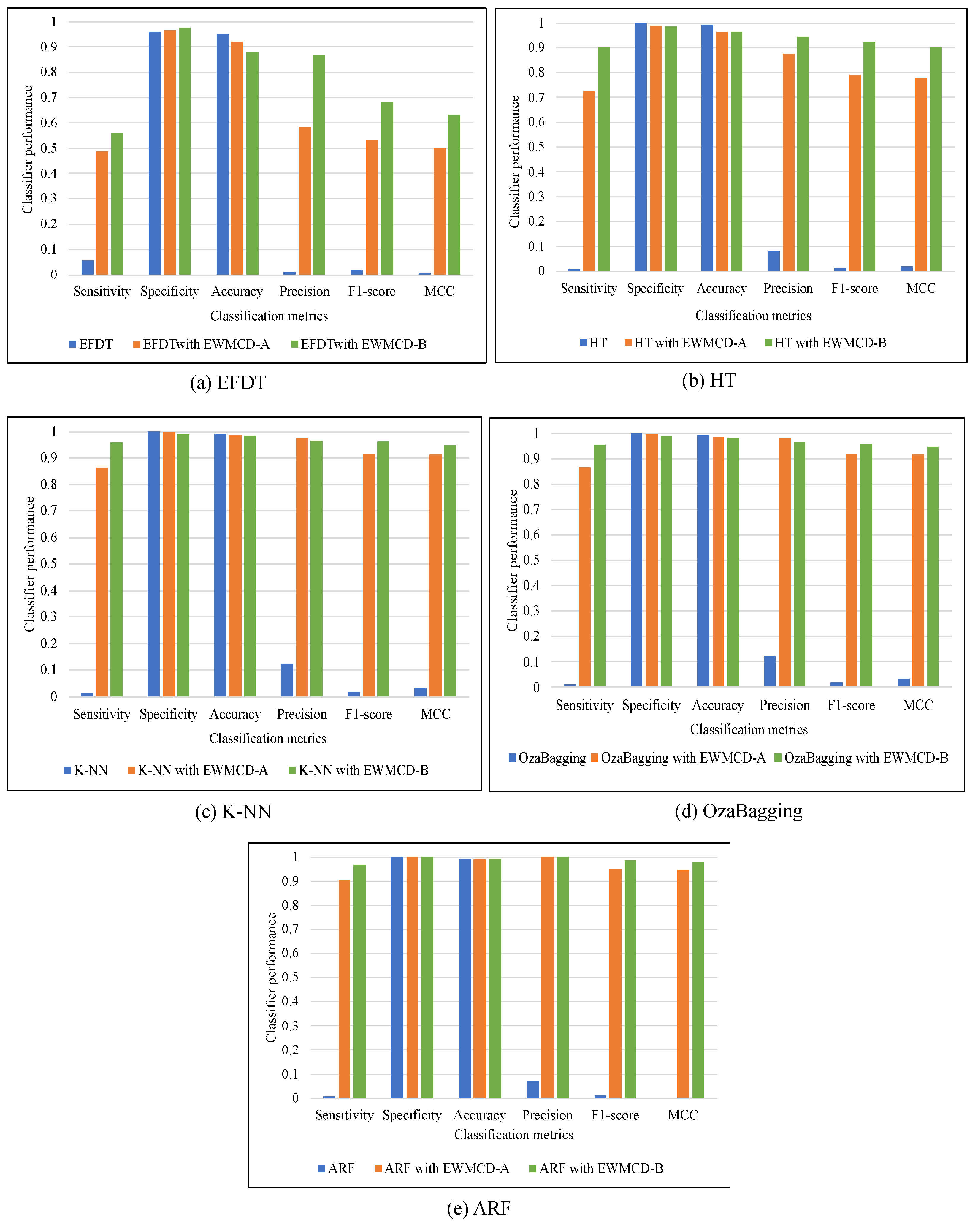
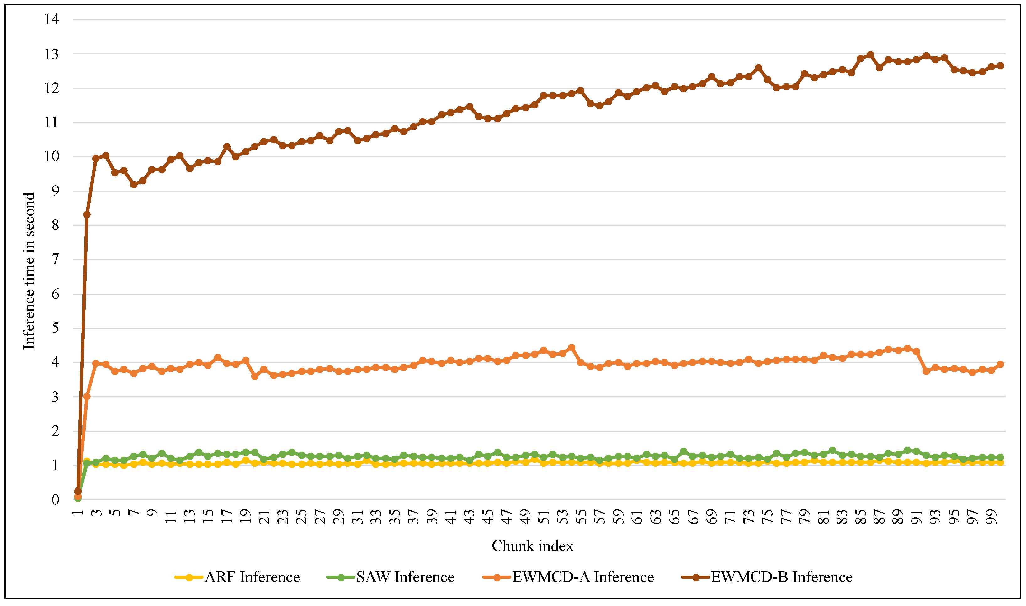
4. Implementation and Results
4.1. Dataset and Framework Description
4.2. Experimental Results
5. Discussion
- Both models, EWMCD-A and EWMCD-B, are designed to work with imbalanced binary-class tasks, which have only two classes, one of which has the majority. The generalization of its work for multi-class classification needs a modification in selecting MCD items due to the possibility of the existence of more than one rare class and, therefore, the multiplicity of clusters and their centroids. However, using the one-versus-all OVA strategy, the proposed model can be used for the multi-class task without more modification.
- The methodology assumes that all features have numerical values for distance calculations. Applying it to categorical features needs additional preprocessing steps, such as data discretization and binarization.
- The accumulated increase in the number of rare-class samples due to the continuous oversampling may cause a reversal of the classes’ probabilities (i.e., the positive class becomes the major one). This inversion can reduce the efficiency of the adaptive classifier. Therefore, the methodology needs a mechanism to prevent the dominance of the rare class after a period of time from the beginning of the classification process.
- Increasing the number of rare-class samples causes distance computation enlargement, consequently, more classifier adapting time. Models’ efficiency can be enhanced by applying algorithm optimization and parallel and distributed processing techniques.
- The proposed methodology is designed for an instance-labeling environment where the actual value of the class is available immediately or shortly after the inference. The method needs more improvement to handle the delayed-labeling environment.
- Regarding the drift of the data distribution, the extreme sensitivity to this drift by the EWMCD-A model leads to the loss of the accumulated number of rare-class instances and, thus, less stability of the classifier. Despite the good performance of the proposed models, the nature of the EEG data do not contain periodic changes between the positive and negative classes during a specific time, and the effectiveness of these models may decrease with other data types that include a continuous difference between two or more classes, such as human activity data. The EWMCD-B model provided a more stable performance and was less affected by data distribution drift, which may make it more suitable for this type of data.
6. Conclusions
Author Contributions
Funding
Institutional Review Board Statement
Informed Consent Statement
Data Availability Statement
Conflicts of Interest
Abbreviations
| EWMCD | Elastic Window based on Minimizing Cluster Distortion |
| EEG | Electroencephalography |
| ADWIN | Adaptive Windowing |
| SMOTE | Synthetic Minority Oversampling Technique |
| VFDT | Very Fast Decision Tree |
| EFDT | Extreme Fast Decision Tree |
| SAW | Similarity-based Adaptive Window |
| VC | Virtual Cluster |
| PIA | Positive Instance Age |
| ARF | Adaptive random forest |
| TNR | True Negative Rate |
| TPR | True Positive Rate |
| FPR | False Positive Rate |
| FNR | False Negative Rate |
References
- Ma, Y.; He, H. Imbalanced Learning: Foundations, Algorithms, and Applications; Wiley: New York, NY, USA, 2013. [Google Scholar]
- Fernández, A.; García, S.; Galar, M.; Prati, R.C.; Krawczyk, B.; Herrera, F. Learning from Imbalanced Data Sets; Springer: Berlin, Germany, 2018; Volume 10. [Google Scholar]
- Nguyen, H.M.; Cooper, E.W.; Kamei, K. Online learning from imbalanced data streams. In Proceedings of the IEEE International Conference of Soft Computing and Pattern Recognition (SoCPaR), Dalian, China, 14–16 October 2011; pp. 347–352. [Google Scholar]
- Du, H.; Zhang, Y.; Gang, K.; Zhang, L.; Chen, Y.C. Online ensemble learning algorithm for imbalanced data stream. Appl. Soft Comput. 2021, 107, 107378. [Google Scholar] [CrossRef]
- Gama, J. Knowledge Discovery from Data Streams; CRC Press: Boca Raton, FL, USA, 2010. [Google Scholar]
- Fatlawi, H.K.; Kiss, A. Similarity-Based Adaptive Window for Improving Classification of Epileptic Seizures with Imbalance EEG Data Stream. Entropy 2022, 24, 1641. [Google Scholar] [CrossRef] [PubMed]
- Leskovec, J.; Rajaraman, A.; Ullman, J.D. Mining of Massive Data Sets; Cambridge University Press: Cambridge, UK, 2020. [Google Scholar]
- Han, J.; Pei, J.; Tong, H. Data Mining: Concepts and Techniques; Morgan kaufmann: Burlington, MA, USA, 2022. [Google Scholar]
- Li, Z.; Huang, W.; Xiong, Y.; Ren, S.; Zhu, T. Incremental learning imbalanced data streams with concept drift: The dynamic updated ensemble algorithm. Knowl.-Based Syst. 2020, 195, 105694. [Google Scholar] [CrossRef]
- Chawla, N.V.; Bowyer, K.W.; Hall, L.O.; Kegelmeyer, W.P. SMOTE: Synthetic minority over-sampling technique. J. Artif. Intell. Res. 2002, 16, 321–357. [Google Scholar] [CrossRef]
- Gulowaty, B.; Ksieniewicz, P. SMOTE algorithm variations in balancing data streams. In Intelligent Data Engineering and Automated Learning—IDEAL 2019; Yin, H., Camacho, D., Tino, P., Tallón-Ballesteros, A., Menezes, R., Allmendinger, R., Eds.; IDEAL 2019. Lecture Notes in Computer Science; Springer: Cham, Switzerland, 2019; Volume 11872, pp. 305–312. [Google Scholar] [CrossRef]
- Chen, B.; Xia, S.; Chen, Z.; Wang, B.; Wang, G. RSMOTE: A self-adaptive robust SMOTE for imbalanced problems with label noise. Inf. Sci. 2021, 553, 397–428. [Google Scholar] [CrossRef]
- Han, H.; Wang, W.Y.; Mao, B.H. Borderline-SMOTE: A new over-sampling method in imbalanced data sets learning. In Advances in Intelligent Computing; Huang, D.S., Zhang, X.P., Huang, G.B., Eds.; ICIC 2005. Lecture Notes in Computer Science; Springer: Berlin/Heidelberg, Germany, 2005; Volume 3644, pp. 878–887. [Google Scholar] [CrossRef]
- Bunkhumpornpat, C.; Sinapiromsaran, K.; Lursinsap, C. Safe-level-smote: Safe-level-synthetic minority over-sampling technique for handling the class imbalanced problem. In Advances in Knowledge Discovery and Data Mining; Theeramunkong, T., Kijsirikul, B., Cercone, N., Ho, T.B., Eds.; PAKDD 2009. Lecture Notes in Computer Science; Springer: Berlin/Heidelberg, Germany, 2009; Volume 5476, pp. 475–482. [Google Scholar] [CrossRef]
- Maldonado, S.; Vairetti, C.; Fernandez, A.; Herrera, F. FW-SMOTE: A feature-weighted oversampling approach for imbalanced classification. Pattern Recognit. 2022, 124, 108511. [Google Scholar] [CrossRef]
- Bhatnagar, J. Basic bounds on cluster error using distortion-rate. Mach. Learn. Appl. 2021, 6, 100160. [Google Scholar] [CrossRef]
- Marutho, D.; Handaka, S.H.; Wijaya, E.; Muljono. The determination of cluster number at k-mean using elbow method and purity evaluation on headline news. In Proceedings of the 2018 International Seminar on Application for Technology of Information and Communication, Semarang, Indonesia, 21–22 September 2018; pp. 533–538. [Google Scholar]
- Et-taleby, A.; Boussetta, M.; Benslimane, M. Faults detection for photovoltaic field based on k-means, elbow, and average silhouette techniques through the segmentation of a thermal image. Int. J. Photoenergy 2020, 2020, 6617597. [Google Scholar] [CrossRef]
- Umargono, E.; Suseno, J.E.; Gunawan, S.V. K-means clustering optimization using the elbow method and early centroid determination based on mean and median formula. In Proceedings of the 2nd International Seminar on Science and Technology (ISSTEC 2019), Yogyakarta, Indonesia, 25–26 November 2019; Atlantis Press: Dordrecht, The Netherlands, 2020; pp. 121–129. [Google Scholar]
- Shi, C.; Wei, B.; Wei, S.; Wang, W.; Liu, H.; Liu, J. A quantitative discriminant method of elbow point for the optimal number of clusters in clustering algorithm. EURASIP J. Wirel. Commun. Netw. 2021, 2021, 1–16. [Google Scholar] [CrossRef]
- Lin, W.C.; Tsai, C.F.; Hu, Y.H.; Jhang, J.S. Clustering-based undersampling in class-imbalanced data. Inf. Sci. 2017, 409, 17–26. [Google Scholar] [CrossRef]
- Tsai, C.F.; Lin, W.C.; Hu, Y.H.; Yao, G.T. Under-sampling class imbalanced datasets by combining clustering analysis and instance selection. Inf. Sci. 2019, 477, 47–54. [Google Scholar] [CrossRef]
- Krawczyk, B.; Koziarski, M.; Woźniak, M. Radial-based oversampling for multiclass imbalanced data classification. IEEE Trans. Neural Netw. Learn. Syst. 2019, 31, 2818–2831. [Google Scholar] [CrossRef] [PubMed]
- Bernardo, A.; Gomes, H.M.; Montiel, J.; Pfahringer, B.; Bifet, A.; Della Valle, E. C-smote: Continuous synthetic minority oversampling for evolving data streams. In Proceedings of the 2020 IEEE International Conference on Big Data (Big Data), Atlanta, GA, USA, 10–13 December 2020; pp. 483–492. [Google Scholar]
- Zyblewski, P.; Sabourin, R.; Woźniak, M. Preprocessed dynamic classifier ensemble selection for highly imbalanced drifted data streams. Inf. Fusion 2021, 66, 138–154. [Google Scholar] [CrossRef]
- Grzyb, J.; Klikowski, J.; Woźniak, M. Hellinger distance weighted ensemble for imbalanced data stream classification. J. Comput. Sci. 2021, 51, 101314. [Google Scholar] [CrossRef]
- Han, M.; Zhang, X.; Chen, Z.; Wu, H.; Li, M. Dynamic ensemble selection classification algorithm based on window over imbalanced drift data stream. Knowl. Inf. Syst. 2022. [Google Scholar] [CrossRef]
- Liu, Y.; Yang, G.; Qiao, S.; Liu, M.; Qu, L.; Han, N.; Wu, T.; Yuan, G.; Peng, Y. Imbalanced data classification: Using transfer learning and active sampling. Eng. Appl. Artif. Intell. 2023, 117, 105621. [Google Scholar] [CrossRef]
- Detti, P. Siena Scalp EEG Database (version 1.0.0). PhysioNet 2020. [Google Scholar] [CrossRef]
- Detti, P.; Vatti, G.; Zabalo Manrique de Lara, G. EEG Synchronization Analysis for Seizure Prediction: A Study on Data of Noninvasive Recordings. Processes 2020, 8, 846. [Google Scholar] [CrossRef]
- Chicco, D.; Jurman, G. The advantages of the Matthews correlation coefficient (MCC) over F1 score and accuracy in binary classification evaluation. BMC Genom. 2020, 21, 1–13. [Google Scholar] [CrossRef]
- Jiang, L.; He, J.; Pan, H.; Wu, D.; Jiang, T.; Liu, J. Seizure detection algorithm based on improved functional brain network structure feature extraction. Biomed. Signal Process. Control. 2023, 79, 104053. [Google Scholar] [CrossRef]
- Dissanayake, T.; Fernando, T.; Denman, S.; Sridharan, S.; Fookes, C. Geometric Deep Learning for Subject Independent Epileptic Seizure Prediction Using Scalp EEG Signals. IEEE J. Biomed. Health Inform. 2021, 26, 527–538. [Google Scholar] [CrossRef] [PubMed]
- Sánchez-Hernández, S.E.; Salido-Ruiz, R.A.; Torres-Ramos, S.; Román-Godínez, I. Evaluation of Feature Selection Methods for Classification of Epileptic Seizure EEG Signals. Sensors 2022, 22, 3066. [Google Scholar] [CrossRef] [PubMed]


| Technique/Metric | EFDT | Hoeffding Tree | K-NN | OzaBagging | ARF |
|---|---|---|---|---|---|
| Sensitivity | 0.4876 | 0.7242 | 0.8642 | 0.8677 | 0.9053 |
| Specificity | 0.9646 | 0.9892 | 0.9979 | 0.9981 | 0.9998 |
| Accuracy | 0.9207 | 0.9639 | 0.9853 | 0.9857 | 0.9909 |
| Precision | 0.5824 | 0.8757 | 0.9768 | 0.9798 | 0.9983 |
| F1-score | 0.5308 | 0.7927 | 0.9170 | 0.9203 | 0.9495 |
| MCC | 0.5019 | 0.7783 | 0.9109 | 0.9144 | 0.9459 |
| Technique/Metric | EFDT | Hoeffding Tree | K-NN | OzaBagging | ARF |
|---|---|---|---|---|---|
| Sensitivity | 0.5594 | 0.9023 | 0.9566 | 0.9551 | 0.9683 |
| Specificity | 0.9745 | 0.9836 | 0.9890 | 0.9891 | 0.9999 |
| Accuracy | 0.8776 | 0.9646 | 0.9814 | 0.9812 | 0.9925 |
| Precision | 0.8697 | 0.9440 | 0.9638 | 0.9640 | 0.9996 |
| F1-score | 0.6808 | 0.9227 | 0.9602 | 0.9595 | 0.9837 |
| MCC | 0.6322 | 0.9001 | 0.9480 | 00.9473 | 0.9790 |
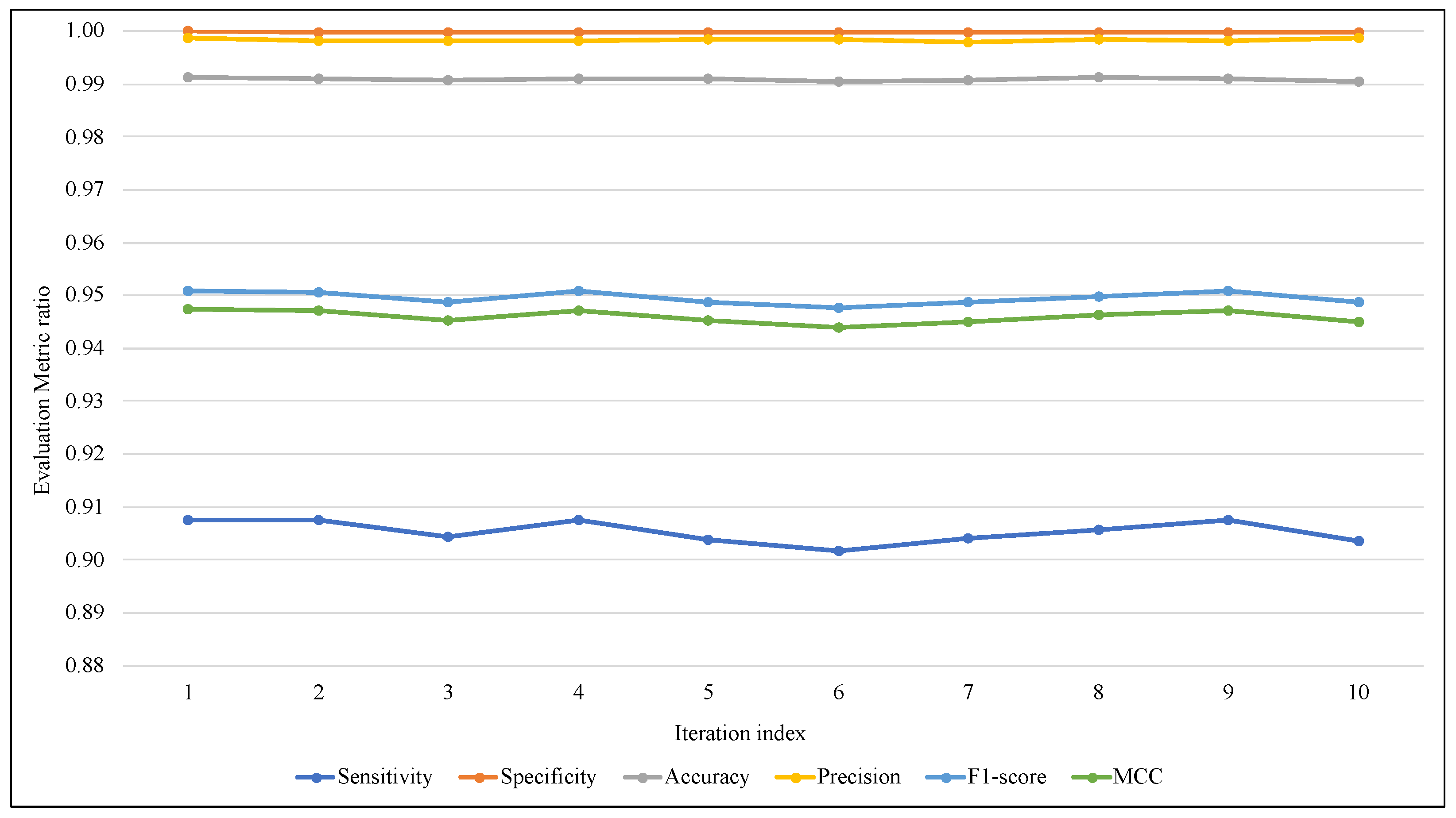
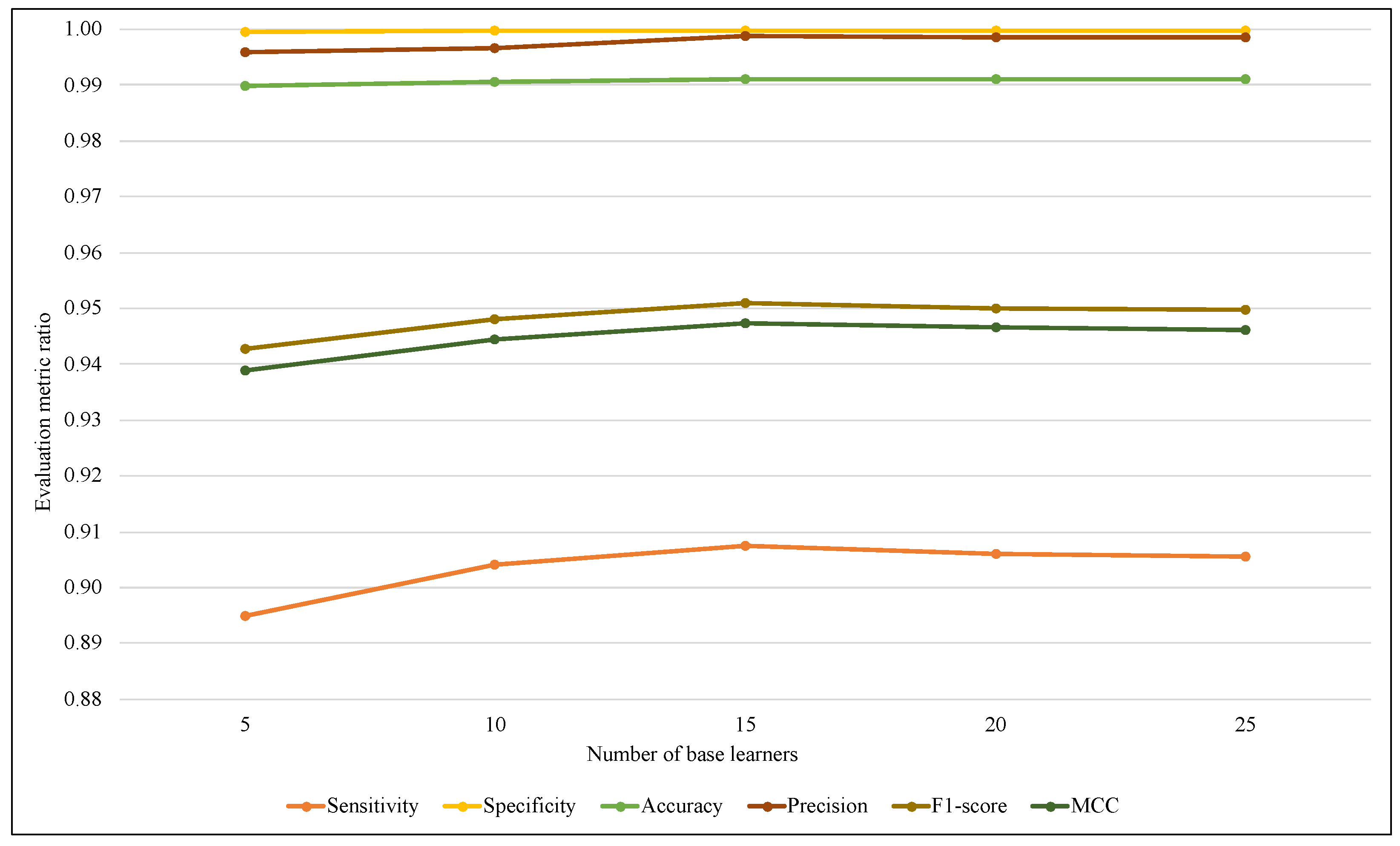
| Technique/Metric | ARF | ARF+SAW | ARF + EWMCD-A | ARF + EWMCD-B |
|---|---|---|---|---|
| Sensitivity | 0.0067 | 0.9313 | 0.9053 | 0.9683 |
| Specificity | 0.9998 | 0.9666 | 0.9998 | 0.9999 |
| Accuarcy | 0.9912 | 0.9644 | 0.9909 | 0.9925 |
| Precision | 0.0700 | 0.6418 | 0.9983 | 0.9996 |
| F1-score | 0.0122 | 0.7600 | 0.9495 | 0.9837 |
| MCC | 0.0000 | 0.7565 | 0.9459 | 0.9790 |
| Model/Metric | EWMCD-A | EW-MCD-B | ||||
|---|---|---|---|---|---|---|
| [0–0.5] | [0.5–1] | [0–1] | [0–0.5] | [0.5–1] | [0–1] | |
| Sensitivity | 0.9260 | 0.9027 | 0.9075 | 0.9702 | 0.9760 | 0.9683 |
| Specificity | 0.9998 | 0.9998 | 0.9999 | 0.9999 | 0.9998 | 0.9999 |
| Accuracy | 0.9913 | 0.9902 | 0.9911 | 0.9924 | 0.9931 | 0.9925 |
| Precision | 0.9987 | 0.9979 | 0.9987 | 0.9998 | 0.9996 | 0.9996 |
| F1-score | 0.9610 | 0.9479 | 0.9509 | 0.9848 | 0.9876 | 0.9837 |
| MCC | 0.9570 | 0.9439 | 0.9473 | 0.9799 | 0.9830 | 0.9790 |
| Articles/ Classification Metric | Accuracy | Sensitivity | Specificity | FPR | FNR |
|---|---|---|---|---|---|
| Detti et al. [32] (2018) | 96.76 | 95.71 | 97.81 | - | - |
| Dissanayakage et al. [33] (2021) | 95.88 | 95.88 | 96.41 | - | - |
| Sánchez-Hernández et al. [34] (2022) | 96 | 76 | - | - | - |
| Jiang et al. [32] (2023) | 95.68 | 97.51 | 93.90 | ||
| EWMCD-A (proposed method) | 99.05 | 90.16 | 99.98 | 00.02 | 09.84 |
| EWMCD-B (proposed method) | 99.25 | 96.82 | 99.99 | 00.01 | 03.18 |
Disclaimer/Publisher’s Note: The statements, opinions and data contained in all publications are solely those of the individual author(s) and contributor(s) and not of MDPI and/or the editor(s). MDPI and/or the editor(s) disclaim responsibility for any injury to people or property resulting from any ideas, methods, instructions or products referred to in the content. |
© 2023 by the authors. Licensee MDPI, Basel, Switzerland. This article is an open access article distributed under the terms and conditions of the Creative Commons Attribution (CC BY) license (https://creativecommons.org/licenses/by/4.0/).
Share and Cite
Fatlawi, H.K.; Kiss, A. An Elastic Self-Adjusting Technique for Rare-Class Synthetic Oversampling Based on Cluster Distortion Minimization in Data Stream. Sensors 2023, 23, 2061. https://doi.org/10.3390/s23042061
Fatlawi HK, Kiss A. An Elastic Self-Adjusting Technique for Rare-Class Synthetic Oversampling Based on Cluster Distortion Minimization in Data Stream. Sensors. 2023; 23(4):2061. https://doi.org/10.3390/s23042061
Chicago/Turabian StyleFatlawi, Hayder K., and Attila Kiss. 2023. "An Elastic Self-Adjusting Technique for Rare-Class Synthetic Oversampling Based on Cluster Distortion Minimization in Data Stream" Sensors 23, no. 4: 2061. https://doi.org/10.3390/s23042061
APA StyleFatlawi, H. K., & Kiss, A. (2023). An Elastic Self-Adjusting Technique for Rare-Class Synthetic Oversampling Based on Cluster Distortion Minimization in Data Stream. Sensors, 23(4), 2061. https://doi.org/10.3390/s23042061