Article

Point Density Variations in Airborne Lidar Point Clouds

1
Center for Geospatial Analytics, North Carolina State University, 2800 Faucette Dr., Campus Box 7106, Raleigh, NC 27695, USA
2
Department of Forestry and Environmental Resources, North Carolina State University, 2820 Faucette Dr., Campus Box 8001, Raleigh, NC 27695, USA
3
Department of Marine, Earth, and Atmospheric Sciences, North Carolina State University, 2800 Faucette Drive, Campus Box 8208, Raleigh, NC 27695, USA
*
Author to whom correspondence should be addressed.
Sensors 2023, 23(3), 1593; https://doi.org/10.3390/s23031593
Submission received: 9 December 2022 / Revised: 26 January 2023 / Accepted: 27 January 2023 / Published: 1 February 2023
(This article belongs to the Special Issue Lidar Remote Sensing for Planetary and Earth Science Applications)

Abstract

:
In spite of increasing point density and accuracy, airborne lidar point clouds often exhibit point density variations. Some of these density variations indicate issues with point clouds, potentially leading to errors in derived products. To highlight these issues, we provide an overview of point density variations and show examples in six airborne lidar point cloud datasets that we used in our topographic and geospatial modeling research. Using the published literature, we identified sources of point density variations and issues indicated or caused by these variations. Lastly, we discuss the reduction in point density variations using decimations, homogenizations, and their applicability.

Graphical Abstract

1. Introduction

Point clouds acquired by airborne lidar have transformed how Earth’s ground surface, vegetation structure, and urban environments are mapped and analyzed. This has led to major advances in terrain modeling, flood prediction, coastal monitoring, forestry and ecosystem studies, and many other disciplines [1,2,3,4]. As with all data collection methods, the process of acquiring point cloud data introduces inconsistencies and errors. Although recent technological advancements aim to minimize the measurement errors, various issues are still present in current datasets. Additionally, datasets captured by legacy systems continue to be a valuable source for many studies detecting long-term changes of the environment [5,6,7,8]. It is, therefore, important to understand errors and anomalies in data acquired by both new and older data acquisition systems to ensure the proper processing, harmonization, and interpretation of point cloud datasets.
Although errors in lidar point clouds were extensively studied [9,10,11,12,13,14] and local variations of point density were recognized in the literature [15,16,17,18,19,20,21], there is less emphasis on studying these density variations and their potential impact on derived products [22,23,24,25,26,27]. Understanding point density variations is important, as lidar point cloud density measurements are used in numerous applications, such as estimating biomass [28], forest fuel mapping [29,30,31], subcanopy solar radiation modeling [32], and mapping forest structures [3,33,34,35,36]. Furthermore, products derived from point clouds such as 3D meshes and digital elevation models (DEMs) are influenced by the presence and absence of points [37]. Lastly, density anomalies may be an indicator of errors in point elevations and issues with other properties of the point cloud, such as missing or vertically unaligned swaths.
In this work, we provide an overview of point density variations and associated errors in airborne lidar point clouds, and discuss their impact on the derived products. We demonstrate the variations using six point cloud datasets (Table 1) used in our topographic and geospatial modeling research [5,33,38,39,40,41]: North Carolina (NC) Floodplain Mapping, 2015 [42], Wake County, 2013 [43], Nantahala 2009 by the National Center for Airborne Laser Mapping (NCALM) [44], and three coastal mapping datasets by NOAA, NASA, and USGS from 1999, 2003, and 2008 [45,46,47]. We reference the current literature to support the examination of the datasets, and to identify potential sources of density variations. Lastly, we discuss decimation and homogenization approaches for reducing point density variations and their appropriate use.

2. Point Density Variations

In an idealized case [48,49,50], an aircraft flies at a constant speed, direction, and altitude above ground level with zero roll, pitch, and yaw, and a known position. A line scanner aboard the aircraft scans the mapped area in the direction perpendicular to the line of flight. The scanner instantly captures a complete scan line with constant spacing between the points on the ground. The speed of the aircraft is constant to ensure that the point spacing in the scan line is the same as the spacing between the scan lines (Figure 1). Lastly, the aircraft flies in straight parallel lines separated by the width of the scan line (swath or flight strip), so that the individual swaths have minimal overlap, and cover the surveyed area without gaps. For a flat terrain without vegetation or other objects, the result would be a regular grid of points. However, none of these idealized procedures is fulfilled in real world conditions. Scanner type, flight plan execution, environmental conditions, data georeferencing, and the presence of vegetation and ground structures all influence airborne lidar data acquisition and the resulting variations in point density. The following paragraphs describe common density variations and related errors for airborne lidar point clouds.

2.1. Scan Patterns

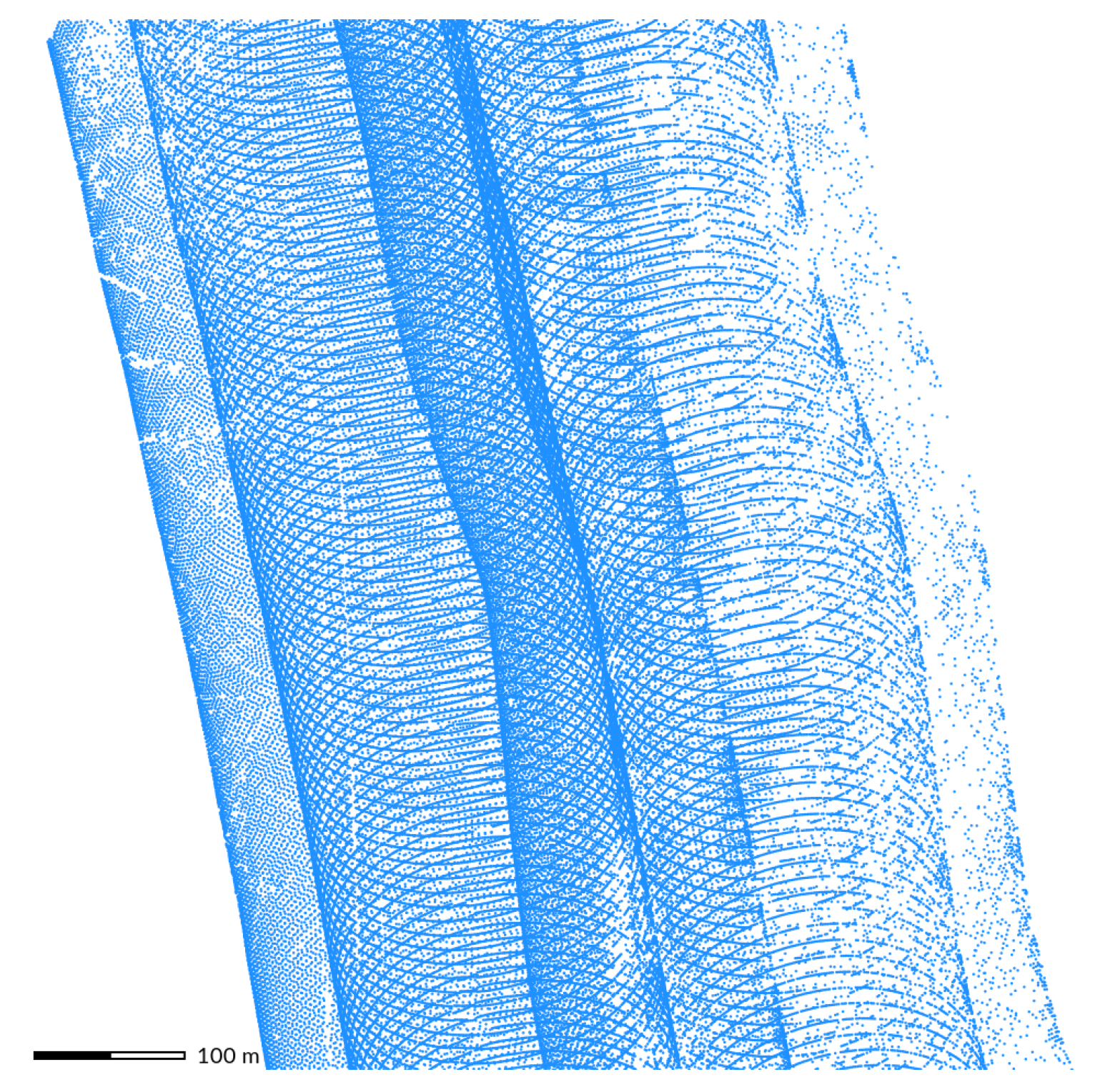
The spatial pattern of points is largely dependent on the type of scanner (Table 2, Figure 2). Rotating mirror scanners and oscillating mirror scanners produce parallel scan lines (assuming constant flight direction) or a zigzag line [51]. While parallel scan lines result in equal point density (Figure 2a,b), a zigzag line always results in variable point density (Figure 2c). Fiber scanners capture the whole scan line at once, producing parallel scan lines that are perpendicular to the flight direction, thus potentially leading to more uniform point distribution [49,52]. Scanners with conical (elliptical) scan patterns (Figure 2d), such as Palmer scanners and some single-photon scanners, measure with a constant scan angle in all directions [53,54,55]. Consequently, each location is scanned twice from different angles, and the conical pattern causes very high density on the edges of each swath unless the scanner accounts for that by changing the speed of scanning. The 1999 dataset by NOAA/NASA/USGS [45] had several overlapping swaths, but clearly shows a conical (elliptical) pattern and the resulting high point density on the swath edges (Figure 3).

2.2. Variations along Scan Line

Point spacing in the direction of a scan line is influenced by the inner working of the scanner and is another source of scanning-related point density variations (Table 2). Older line scanners usually scan in equal angle steps, which results in higher point density in the middle of the scan line, and lower density toward the ends of the scan line [49]. On the other hand, newer scanners can achieve equal point spacing in the middle of the scan line, but anomalies can still occur at the end of a scan line due to the acceleration of the inner mechanical parts of mirror scanners. For example, the NC Floodplain Mapping Program dataset exhibited higher point density at the end of the scan line (Figure 4).

2.3. Banding

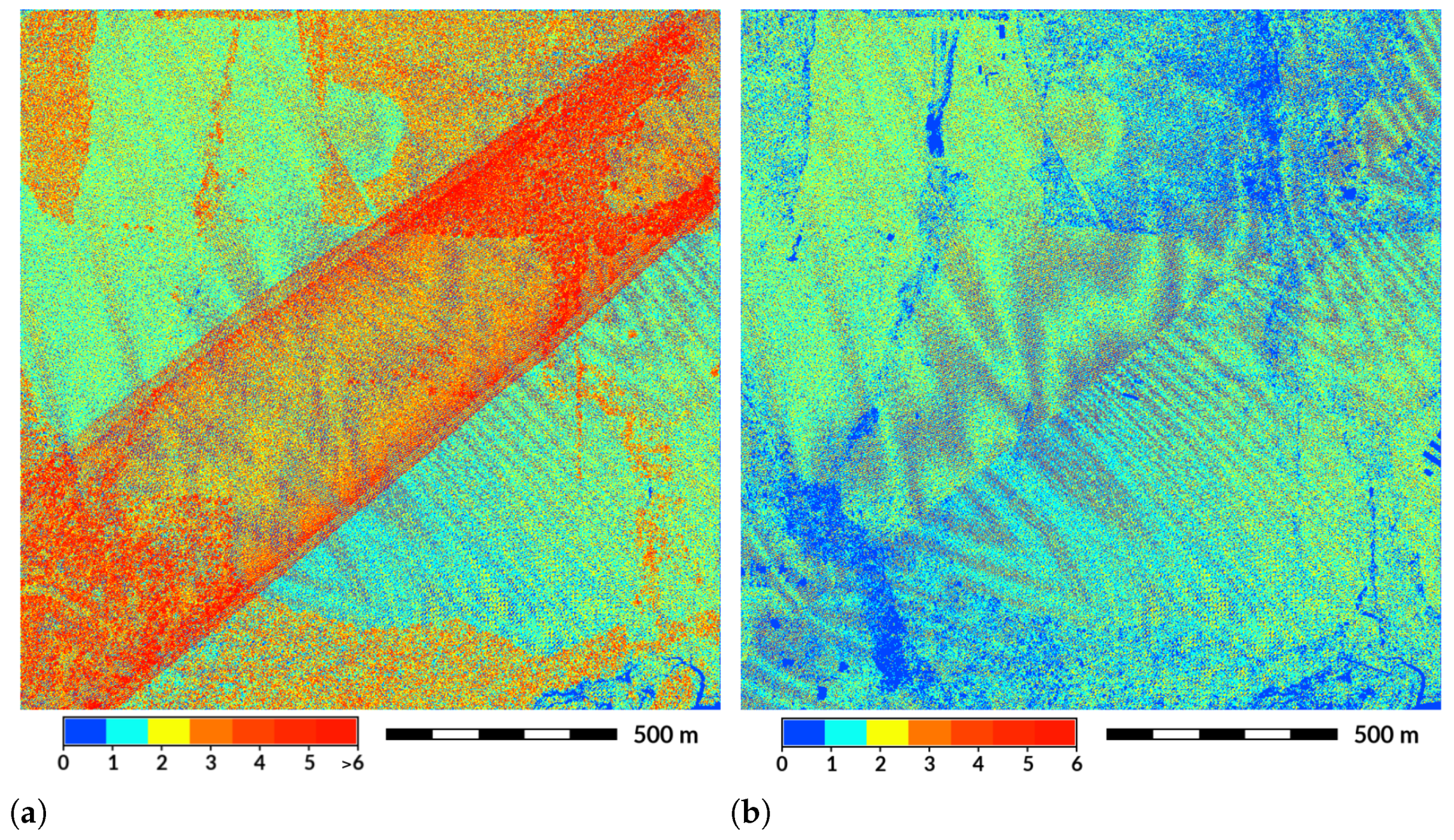
Lidar scanners are usually synchronized with the speed of the aircraft to achieve constant density in all directions [56]. However, variable aircraft speed due to wind, when not accounted for by the scanner, results in stripes of higher and lower densities along the flight line [56]. These periodical changes in densities are called banding [37] and can be observed easily by computing the number of points per grid cell. Such an examination of the NCALM and NOAA datasets shows strong banding effect (Figure 5). To mediate speed-related banding, helicopters may be used to obtain high-resolution coverage with more uniform distribution of points because they can more easily control their speed [57].
Another cause of banding is a change in the pitch of the aircraft. In addition to irregular point density, this can also cause errors in measured elevation [37]. When the pitch value recorded by the navigation system is different from the actual pitch, the resulting point is assigned an incorrect position, causing artificially undulating terrain. To determine if the banding is just in density or also in elevation, the DEM can be compared to another DEM or a profile of the point density and the DEM can be examined.

2.4. Variations Due to Aircraft Altitude Variations

Point density is also influenced by the altitude of the aircraft above ground or sea level [58]. A lower altitude causes smaller point spacing in the scan line, resulting in variable point density when the aircraft altitude varies during the flight. Additionally, too low altitude may cause a swath to be too narrow to overlap with or touch an adjacent swath. For some scanners, such as those with an elliptical scan pattern, changes in altitude also influence spacing in the flight direction. For line scanners, the dynamically adjusted speed of scanning based on the altitude can mitigate density variations in all directions.
In mountainous areas, the changes of terrain elevation together with a constant altitude (height above sea level) of the aircraft cause variable densities in the higher and lower situated areas when the sensor is not adjusted. Similarly, steep slopes result in fewer points capturing the surface. Although the horizontal density stays the same in this case, there are fewer points covering a given surface in a sloped area in comparison to a flat area.

2.5. Swath Overlaps

Airborne lidar point clouds are collected in parallel swaths (passes). To ensure that there are no gaps in between swaths, individual swaths usually overlap, as in the Wake County [43] dataset (Figure 6 and Figure 7). Another reason for collecting overlapping swaths is to mitigate errors introduced by the acquisition of the position and orientation of the aircraft, which are used to derive point coordinates. Collecting swaths with overlap generates redundant information that can be used to align individual swaths by eliminating the horizontal and vertical time-dependent shifts [48]. These shifts, occurring due to systematic navigation system errors, can then be minimized via, for example, least-squares matching [56,59]. However, swath overlaps are a significant source of point density variations [60,61]. Therefore, overlaps are often removed from the dataset, especially if classification is performed, for example, classified ground points in the Wake County dataset do not include any swath overlaps (Figure 7). Although overlap removal eliminates the issue of higher point density, the new issue of having abrupt changes in the point density patterns arises.
For vegetation-related metrics, such as the subcanopy solar radiation model [32], any variable point density at the swath overlap may be an issue. For example, the NCALM dataset had two sets of north–south swaths overlapping each other (Figure 8). As a result, the dataset contains areas with high point density caused by two or more swaths overlapping and areas with low point density caused by a gap in between the swaths in one of the sets. Derived skewness of point elevations, used in forestry applications [62], then shows both actual features (e.g., vegetation types) and artifacts representing the gaps (Figure 8).
For terrain reconstruction, an abrupt change in density between two swaths may highlight an abrupt change in point elevations that are a result of uncorrected errors in positioning [63]. A positioning error that was not corrected by aligning swaths resulted in a flawed terrain reconstruction using the Wake County dataset. In the dataset, an abrupt change in elevation corresponds to an abrupt change in the point density pattern and is visible on the shaded relief model and when the dataset is compared with the NC Floodplain Mapping Program dataset (Figure 9). This is an issue for further time series analysis because it prevents direct comparison of time steps. The flawed terrain reconstruction causes issues for further analysis. For example, simulated water flow may follow the abrupt change in elevation instead of the actual terrain (Figure 9c).
Furthermore, the width of swath overlaps may vary. While modern scanning systems try to adjust the scan line and apply on-board checks, changes in the aircraft’s altitude and roll, and navigation errors may lead to overlap width variations or gaps (Table 2). Lastly, a difference in the number of swaths can cause point density differences between otherwise comparable datasets [64].

2.6. Moiré and Corduroy Effects

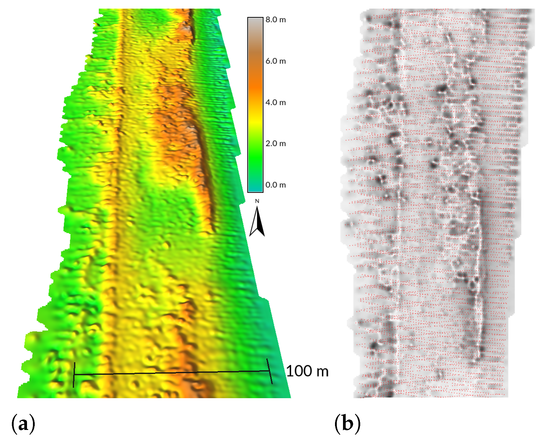
When the number of points per grid cell is computed to spatially analyze the point density, the overlap of the grid pattern and the point pattern may cause a Moiré effect (pattern) in the resulting image of point density [66,67,68]. Wake County dataset shows the Moiré effect in the point density of classified ground points (Figure 7b). Additionally, when two alternating series of scan lines overlap as a result of swath overlap, scanning back and forth with a line scanner, or doubled scan pattern, a detailed digital elevation model contains stripes of higher and lower elevation when the points are not accurately georeferenced [66,69,70]. This Corduroy effect can be observed in the NASA/USGS dataset where two sets of scan lines cause corduroy lines in the east-west direction (Figure 10). While the corduroy effect can be grouped together with the Moiré effect into oscillatory patterns [50], unlike Moiré, the corduroy effect is associated with elevations of points rather than just their positions in relation to a 2D grid.

2.7. Surface Material Properties and Obstructions

Other commonly recognized sources of lower densities or gaps in point clouds are signal noise, surfaces absorbing the pulses, and small obstructing objects such as small details on building roofs [72]. Depending on the wavelength used by the lidar sensor, some surfaces, mainly water and dark asphalt, return a weaker signal or do not return any pulses, which results in lower point return intensities or no recorded points at all. The surfaces that are most likely to suffer from these issues are water bodies, wetlands, and some types of roads and roofs. Examples from the Wake County dataset show almost no points for a water body and reduced number of points for a specific building roof (Figure 11).

2.8. Variations Due to Vegetation

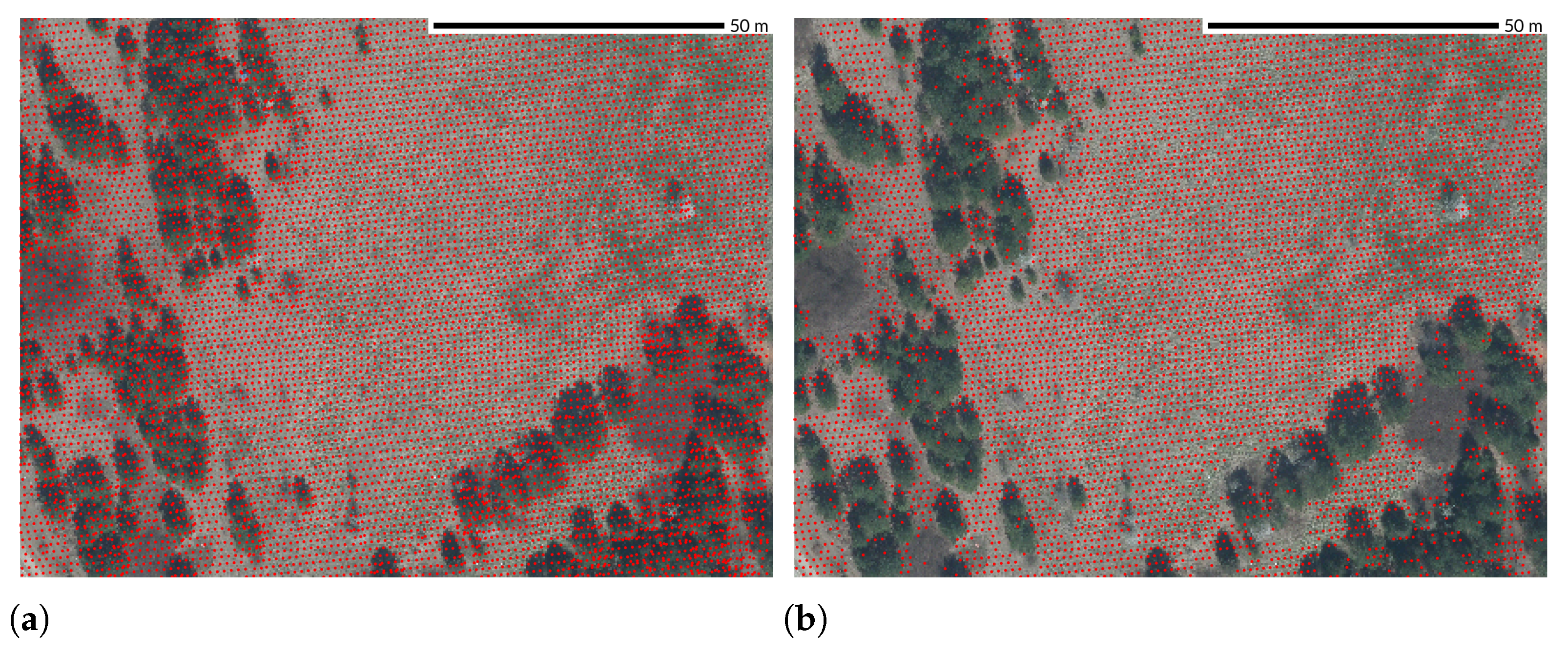
Density and spatial distribution of points in vegetated areas typically differ from nonvegetated areas due to occlusion or multiple returns in the canopy as opposed to a single return from the bare ground [53,62]. For example, the NC Floodplain Mapping Program dataset had a regular point pattern in nonvegetated areas; in vegetated areas, distribution is irregular, and classified ground points have lower density (Figure 12).
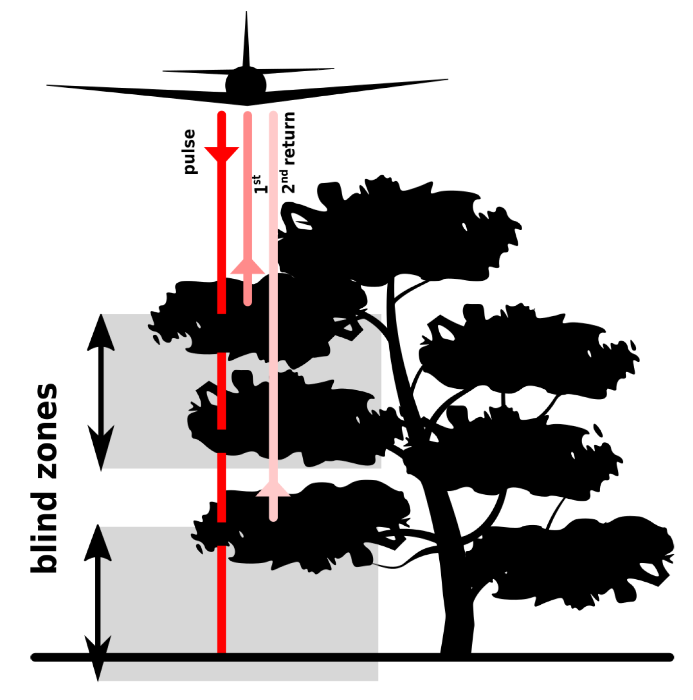
Point density is also variable in the vertical direction depending on several factors related to the structure of vegetation (which can be used for classification). For example, a planted forest is characterized by significantly skewed distributions in comparison to a natural one [73] that is visible on a transect from the NC Floodplain Mapping Program dataset (Figure 13). In the natural forest, lidar pulses penetrate the canopy and reveal complex structure and understory (Figure 13, left). In the planted forest, most of the points are concentrated in the canopy suggesting thick canopy and no understory, given the presence of the ground points (Figure 13, right). This difference can be used for classification to distinguish these two forest types. The forest type also influences the wintertime and summertime rates of penetration through the canopy [48]. Lastly, a so-called blind zone may cause gaps in vertical point distribution [63]. A blind zone is a distance where no subsequent returns are recorded after a previously recorded return due to a limited response time of the detector (Figure 14). For example, lidar sensor Leica ALS80-HP reports a blind zone distance of 2.8 m [74].

2.9. Ground Points

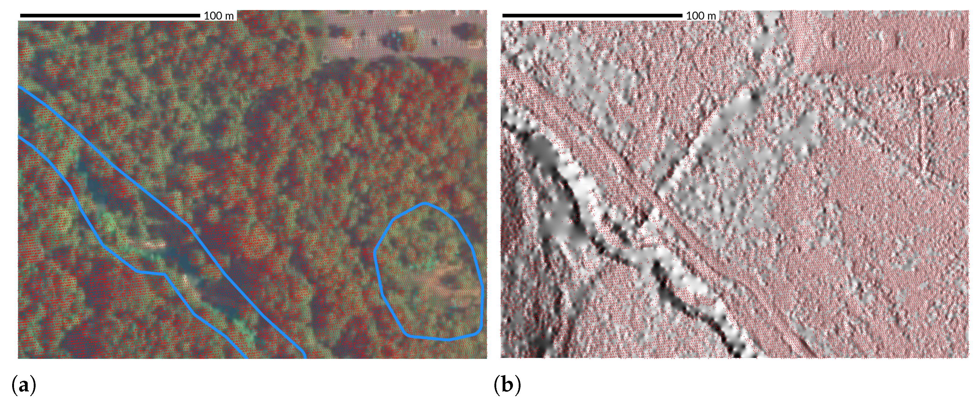
The NC Floodplain Mapping Program dataset demonstrated that points classified as ground may have much higher variability in both pattern and overall density compared to the variability of all points in the point cloud. (Figure 12). Depending on the vegetation density, fewer pulses penetrate the vegetation all the way to the ground, resulting in lower ground point density in vegetated areas than that in nonvegetated areas [48,53]. The gaps may also be caused by buildings or objects that do not reflect the pulses. The interpolation of these gaps to derive a digital terrain model (DTM) representing ground surface results in smooth areas where the level of detail is generally lower than that in areas with full point coverage (Figure 15). Additionally, ground points classified by data providers often have points from overlapping swaths (scan lines) removed as in the case of Wake County dataset (Figure 7). Together with other ground point density variations, such as abrupt changes (Figure 9) or banding (Figure 5), occlusion-caused gaps (Figure 15) may indicate an issue with accuracy of resulting DTMs (Table 3).

2.10. Redundant Points

Point redundancy, i.e., whether certain points in a dataset are needed, depends on a particular application rather than being an inherent property of a point cloud. Point redundancy can be a result of several aforementioned local density variations such as scan line anomalies (Figure 4), banding (Figure 5), and swath overlaps (Figure 9). Additionally, modern sensors generate point cloud densities that exceed the needs of most applications resulting in evenly distributed redundant points, for example, a Geiger-mode sensor may produce 25 points per square meter [54]. Lastly, when combining multiple adjacent point clouds with inconsistent point densities into one spatially continuous dataset or multiple overlapping point clouds with inconsistent densities into a time series, points in higher density point clouds would be considered redundant.
For the creation of DTMs, the minimal point density depends on the desired resolution of the surface [75]. Even though high-precision DTMs generally do not need the full density of the current point cloud [24,40,76,77,78,79], redundant points do not negatively influence the resulting DTM. However, redundant points can significantly increase the processing time or storage requirements [80,81,82], causing practical issues for many applications.

3. Reducing Point Density Variations in Point Clouds

Point density variations in point cloud datasets, including point redundancy, can be mitigated or removed using various decimation and homogenization techniques. While decimation removes redundant points, homogenization makes point distribution more uniform. Both approaches are commonly used during point cloud processing to improve the point cloud properties for a particular application.

3.1. Applicability of Decimation and Homogenization

Decimation, also referred to as thinning, downsampling, or simplification, is a reduction in the number of points in a point cloud that preserves selected properties of the point cloud. While many decimations lead to homogenization of the point density across a point cloud, full or true homogenization may include adding points where density is low, i.e., filling. Decimations and homogenizations can be applied to one or more point clouds to harmonize point densities across a time series or spatially adjacent datasets.
Given the prevalence of point density variations, algorithms working with point clouds should consider the effect of these variations [72,83]. However, not all applications can or need to remove the density variations from the point cloud. For example, such metrics as above-ground biomass (AGB) estimates [28], leaf area density (LAD) distribution [35], subcanopy solar radiation model [32], and the analysis of point density percentiles used as a measure of crown density [36] would be negatively affected by adding or removing points.
Decimation is advantageous for deriving DTMs and other products from point clouds at different resolutions in order to reduce processing time and computing resources needed [81,84,85]. Additionally, decimation can remove density variations resulting from swath overlaps. On the other hand, deriving high resolution digital surface model (DSM) and reconstruction of 3D objects, such as buildings or full 3D models of trees [86,87], may benefit more from higher point density than the creation of (usually smooth) DTMs.
For point cloud classification, high point density is usually advantageous to distinguish ground surface points from points that represent returns from trees, buildings, and other objects [9,14,88], and to preserve sharp edges of the objects such as building roofs.

3.2. Decimation and Homogenization

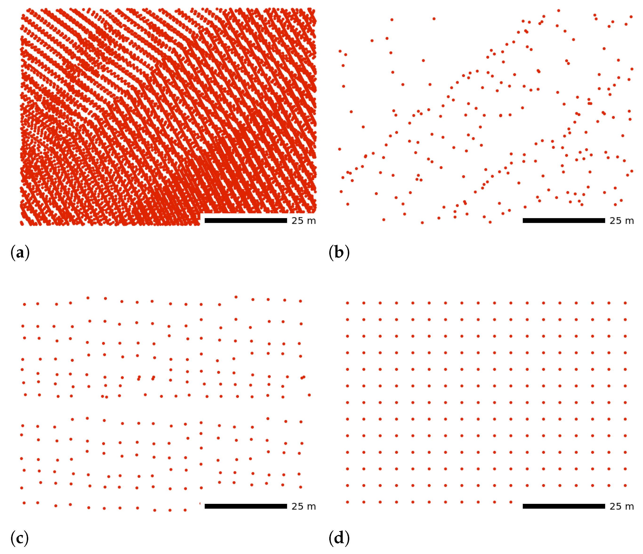
Decimation techniques range from simple ones, such as random sampling, to complex decimations based on shape of the objects described by the point cloud [82,89,90,91,92,93,94,95,96]. Random sampling can be based on the ordinal number of a point within the point cloud (count-based decimation). The resulting point cloud contains only every n-th point, but the overall point distribution remains the same; possibly preserving some of the variations such as higher density at the end of scan lines (Figure 16b). This technique works well for lidar point clouds when points are ordered by collection time and are used for creation of DTMs [97,98].
Grid-based decimation (Figure 16c) is based on binning of the points into a 2D or 3D raster (grid) and is similar to creating a raster image from a point cloud (as opposed to creating a subset of a point cloud). Decimation can also be based on dividing space using kd-trees, quad-trees, oct-trees, or Voronoi diagrams [99,100,101]. These decimations typically work within the neighborhoods of the points and take into account distances between the points, size of the neighborhood, or a number of points in the neighborhood. At the cost of higher complexity, algorithms focused on surfaces and curvatures better preserve objects represented by the point cloud [61,95,102].
Many decimation techniques, such as grid-based decimation, aim at the homogenization of the point density by, e.g., snapping to a grid (Figure 16d). However, decimations can make the distribution of points more regular only in the areas with redundant points. For full homogenization, resampling based on regular grids can add points to areas with low point density [100,101,103].
3D raster (grid) creation or space voxelization, i.e., replacing groups of points by 3D cubes or single points, is used by some 3D metrics and object reconstruction methods to remove redundant points while characterizing, e.g., forest canopy fuel properties [104], internal patterns of vegetation [33], fine-scale bird habitat [105], and detailed tree models [106,107]. These methods often use relative point counts based on absolute point counts in the neighborhood [3,40], thus reducing the overall data and potentially reducing the influence of variable point density in the point cloud.

4. Conclusions

Despite the advancements in airborne lidar technology, different types of point density variations and related errors are common in currently used datasets as the cost of equipment and repeated airborne surveys remains high. To bring attention to these issues, we provided an overview of the different types of density variations that may indicate errors in the acquired data and may lead to artifacts or distortions in the derived products. We demonstrated point density variations and related artifacts by examples from six point cloud datasets and by referenced literature. Further, we discussed how density variations can be reduced in a point cloud by various decimation and homogenization techniques, along with the limitations of those methods.
While some authors include point density analysis [23,25,108,109] or take into account local density variations when processing lidar point clouds [87,103,110,111,112,113,114,115], our overview further highlights the importance of point density analysis as a starting point for studies using lidar point clouds. Special care should be given to point clouds used as input for analytical methods that are highly influenced by point cloud density, such as many vegetation-related metrics.

Author Contributions

Conceptualization, V.P., J.B.M., H.M. and R.K.M.; methodology, V.P. and H.M.; software, V.P.; investigation, V.P. and A.P.; resources, V.P. and R.K.M.; data curation, V.P.; writing—original draft preparation, V.P.; writing—review and editing, V.P., A.P., J.B.M., H.M. and R.K.M.; visualization, V.P. and A.P.; supervision, H.M. and R.K.M.; project administration, V.P. and R.K.M.; funding acquisition, H.M. and R.K.M. All authors have read and agreed to the published version of the manuscript.

Funding

This research received no external funding.

Institutional Review Board Statement

Not applicable.

Informed Consent Statement

Not applicable.

Data Availability Statement

The airborne lidar data we used include NC Quality Level 2 lidar data (NC QL2) for North Carolina, USA collected by North Carolina Floodplain Mapping Program in 2015 [42] and Wake County lidar data for Wake County, North Carolina, USA collected in 2013 [43]. Further, we use coastal lidar data NOAA/NASA/USGS, 1999 [45] collected by National Oceanic and Atmospheric Administration (NOAA), National Aeronautics and Space Administration (NASA), and U.S. Geological Survey (USGS) in September 1999 in a post-Hurricane Floyd survey. The coastal dataset NASA/USGS, 2003 [46] from the pre-hurricane Isabel survey in 2003 was collected with the NASA/USGS Experimental Advanced Airborne Research Lidar (EAARL) [116] and the NOAA, 2008 [47] dataset was collected in March 2008 using the NOAA March Integrated Ocean and Coastal Mapping (IOCM) equipment. The Nantahala 2009 dataset [44] was obtained from OpenTopography. Lidar data acquisition and processing was completed by the National Center for Airborne Laser Mapping (NCALM). NCALM funding was provided by NSF’s Division of Earth Sciences, Instrumentation and Facilities Program EAR-1043051. All datasets are available online except the Wake County dataset, which is available from the Wake County Geographic Information Services (GIS) department. GRASS GIS software [117,118] used to create visualizations and compute densities and decimation is available online under GNU General Public License.

Acknowledgments

We are grateful to the GRASS GIS developer and user community for developing and maintaining GRASS GIS software package that we used to process the data and create the figures. We would like to also acknowledge the creators of the other open source software extensively used in preparation of the manuscript, including, but not limited to, PDAL, Inkscape, Python, Jupyter, Linux, Ubuntu, Kile, LaTeX, and Git. We also acknowledge the authors of Matplotlib color table Viridis, which we used in several figures.

Conflicts of Interest

The authors declare no conflict of interest.

Abbreviations

The following abbreviations are used in this manuscript:
AGBAbove-ground biomass
DEMDigital elevation model
DSMDigital surface model
DTMDigital terrain model
EAARLExperimental Advanced Airborne Research Lidar
IOCMIntegrated Ocean and Coastal Mapping
LADLeaf area density
NASA(U.S.) National Aeronautics and Space Administration
NCALM(U.S.) National Center for Airborne Laser Mapping
NCNorth Carolina, USA
NOAA(U.S.) National Oceanic and Atmospheric Administration
NSF(U.S.) National Science Foundation
QL2Quality Level 2
SIMWESimulation of water and erosion
USGSU.S. Geological Survey
USA (U.S.)United States of America

References

  1. Lefsky, M.A.; Cohen, W.B.; Parker, G.G.; Harding, D.J. Lidar Remote Sensing for Ecosystem Studies. BioScience 2002, 52, 19–30. [Google Scholar] [CrossRef]
  2. Kobal, M.; Bertoncelj, I.; Pirotti, F.; Dakskobler, I.; Kutnar, L. Using Lidar Data to Analyse Sinkhole Characteristics Relevant for Understory Vegetation under Forest Cover—Case Study of a High Karst Area in the Dinaric Mountains. PLoS ONE 2015, 10, e0122070. [Google Scholar] [CrossRef] [PubMed]
  3. Kumar, J.; Weiner, J.; Hargrove, W.W.; Norman, S.P.; Hoffman, F.M.; Newcomb, D. Characterization and classification of vegetation canopy structure and distribution within the Great Smoky Mountains National Park using LiDAR. In Proceedings of the 2015 IEEE International Conference on Data Mining Workshop (ICDMW), Atlantic City, NJ, USA, 14–17 November 2015; pp. 1478–1485. [Google Scholar]
  4. Fisher, J.T.; Erasmus, B.F.; Witkowski, E.T.; Aardt, J.; Wessels, K.J.; Asner, G.P. Savanna woody vegetation classification–now in 3-D. Appl. Veg. Sci. 2014, 17, 172–184. [Google Scholar] [CrossRef]
  5. Hardin, E.; Mitasova, H.; Tateosian, L.; Overton, M. GIS-Based Analysis of Coastal Lidar Time-Series; Springer: New York, NY, USA, 2014. [Google Scholar] [CrossRef]
  6. Hopkinson, C.; Chasmer, L.; Hall, R.J. The uncertainty in conifer plantation growth prediction from multi-temporal lidar datasets. Remote Sens. Environ. 2008, 112, 1168–1180. [Google Scholar] [CrossRef]
  7. Anders, N.S.; Seijmonsbergen, A.C.; Bouten, W. Geomorphological Change Detection Using Object-Based Feature Extraction From Multi-Temporal LiDAR Data. IEEE Geosci. Remote Sens. Lett. 2013, 10, 1587–1591. [Google Scholar] [CrossRef]
  8. Zhao, K.; Suarez, J.C.; Garcia, M.; Hu, T.; Wang, C.; Londo, A. Utility of multitemporal lidar for forest and carbon monitoring: Tree growth, biomass dynamics, and carbon flux. Remote Sens. Environ. 2018, 204, 883–897. [Google Scholar] [CrossRef]
  9. Huising, E.J.; Gomes Pereira, L.M. Errors and accuracy estimates of laser data acquired by various laser scanning systems for topographic applications. ISPRS J. Photogramm. Remote Sens. 1998, 53, 245–261. [Google Scholar] [CrossRef]
  10. Latypov, D. Effects of laser beam alignment tolerance on lidar accuracy. ISPRS J. Photogramm. Remote Sens. 2005, 59, 361–368. [Google Scholar] [CrossRef]
  11. May, N.C.; Toth, C.K. Point positioning accuracy of airborne LiDAR systems: A rigorous analysis. Int. Arch. Photogramm. Remote Sens. Spat. Inf. Sci. 2007, 36, 19–21. [Google Scholar]
  12. Schaer, P.; Skaloud, J.; Landtwing, S.; Legat, K. Accuracy estimation for laser point cloud including scanning geometry. In Proceedings of the Mobile Mapping Symposium, Padova, Italy, 29–31 May 2007. [Google Scholar]
  13. Aguilar, F.J.; Mills, J.P. Accuracy assessment of lidar-derived digital elevation models. Photogramm. Rec. 2008, 23, 148–169. [Google Scholar] [CrossRef]
  14. Anderson, B.C. Assessing Accuracy in Varying LIDAR Data Point Densities in Digital Elevation Maps. Master’s Thesis, Naval Postgraduate School, Monterey, CA, USA, 2008. [Google Scholar]
  15. Biasutti, P.; Bugeau, A.; Aujol, J.F.; Brédif, M. Visibility estimation in point clouds with variable density. In Proceedings of the 14th International Joint Conference on Computer Vision, Imaging and Computer Graphics Theory and Applications, Prague, Czech Republic, 25–27 February 2019. [Google Scholar]
  16. Malinverni, E.S.; Pierdicca, R.; Paolanti, M.; Martini, M.; Morbidoni, C.; Matrone, F.; Lingua, A. Deep learning for semantic segmentation of 3D point cloud. Int. Arch. Photogramm. Remote Sens Spat. Inf. Sci. 2019, XLII-2/W15, 735–742. [Google Scholar] [CrossRef]
  17. Zhou, Y.; Sun, P.; Zhang, Y.; Anguelov, D.; Gao, J.; Ouyang, T.; Guo, J.; Ngiam, J.; Vasudevan, V. End-to-End Multi-View Fusion for 3D Object Detection in LiDAR Point Clouds. In Proceedings of the Conference on Robot Learning, Virtual, 16–18 November; 2020; pp. 923–932. [Google Scholar]
  18. Yu, X.; He, W.; Qian, X.; Yang, Y.; Zhang, T.; Ou, L. Real-time rail recognition based on 3D point clouds. Meas. Sci. Technol. 2022, 33, 105207. [Google Scholar] [CrossRef]
  19. Roynard, X.; Deschaud, J.E.; Goulette, F. Classification of Point Cloud Scenes with Multiscale Voxel Deep Network. arXiv 2018, arXiv:1804.03583. [Google Scholar]
  20. Zhang, Y.; Yang, W.; Liu, X.; Wan, Y.; Zhu, X.; Tan, Y. Unsupervised Building Instance Segmentation of Airborne LiDAR Point Clouds for Parallel Reconstruction Analysis. Remote Sens. 2021, 13, 1136. [Google Scholar] [CrossRef]
  21. Xing, X.F.; Mostafavi, M.A.; Edwards, G.; Sabo, N. An improved automatic pointwise semantic segmentation of a 3D urban scene from mobile terrestrial and airborne LiDAR point clouds: A machine learning approach. ISPRS Ann. Photogramm. Remote Sens. Spat. Inf. Sci. 2019, 4, 139–146. [Google Scholar] [CrossRef]
  22. Wu, J.; Yao, W.; Chi, W.; Zhao, X. Comprehensive quality evaluation of airborne lidar data. In Proceedings of the International Symposium on Lidar and Radar Mapping 2011: Technologies and Applications, International Society for Optics and Photonics, Nanjing, China, 26–29 May 2011; Volume 8286, p. 604. [Google Scholar] [CrossRef]
  23. Dandois, J.P.; Ellis, E.C. High spatial resolution three-dimensional mapping of vegetation spectral dynamics using computer vision. Remote Sens. Environ. 2013, 136, 259–276. [Google Scholar] [CrossRef]
  24. Zhao, C.; Jensen, J.; Deng, X.; Dede-Bamfo, N. Impacts of LiDAR Sampling Methods and Point Spacing Density on DEM Generation. Pap. Appl. Geogr. 2016, 2, 261–270. [Google Scholar] [CrossRef]
  25. Pricope, N.G.; Halls, J.N.; Mapes, K.L.; Baxley, J.B.; Wu, J.J. Quantitative Comparison of UAS-Borne LiDAR Systems for High-Resolution Forested Wetland Mapping. Sensors 2020, 20, 4453. [Google Scholar] [CrossRef]
  26. Cățeanu, M.; Ciubotaru, A. Accuracy of Ground Surface Interpolation from Airborne Laser Scanning (ALS) Data in Dense Forest Cover. ISPRS Int. J. Geo-Inf. 2020, 9, 224. [Google Scholar] [CrossRef]
  27. Jancewicz, K.; Porębna, W. Point cloud does matter. Selected issues of using airborne LiDAR elevation data in geomorphometric studies of rugged sandstone terrain under forest—Case study from Central Europe. Geomorphology 2022, 412, 108316. [Google Scholar] [CrossRef]
  28. Calders, K.; Newnham, G.; Burt, A.; Murphy, S.; Raumonen, P.; Herold, M.; Culvenor, D.; Avitabile, V.; Disney, M.; Armston, J.; et al. Nondestructive estimates of above-ground biomass using terrestrial laser scanning. Methods Ecol. Evol. 2015, 6, 198–208. [Google Scholar] [CrossRef]
  29. Morsdorf, F.; Mårell, A.; Koetz, B.; Cassagne, N.; Pimont, F.; Rigolot, E.; Allgöwer, B. Discrimination of vegetation strata in a multi-layered Mediterranean forest ecosystem using height and intensity information derived from airborne laser scanning. Remote Sens. Environ. 2010, 114, 1403–1415. [Google Scholar] [CrossRef]
  30. Andersen, H.E.; McGaughey, R.J.; Reutebuch, S.E. Estimating forest canopy fuel parameters using LIDAR data. Remote Sens. Environ. 2005, 94, 441–449. [Google Scholar] [CrossRef]
  31. Riaño, D.; Meier, E.; Allgöwer, B.; Chuvieco, E.; Ustin, S.L. Modeling airborne laser scanning data for the spatial generation of critical forest parameters in fire behavior modeling. Remote Sens. Environ. 2003, 86, 177–186. [Google Scholar] [CrossRef]
  32. Bode, C.A.; Limm, M.P.; Power, M.E.; Finlay, J.C. Subcanopy Solar Radiation model: Predicting solar radiation across a heavily vegetated landscape using LiDAR and GIS solar radiation models. Remote Sens. Environ. 2014, 154, 387–397. [Google Scholar] [CrossRef]
  33. Petras, V.; Newcomb, D.J.; Mitasova, H. Generalized 3D fragmentation index derived from lidar point clouds. Open Geospat. Data Softw. Stand. 2017, 2, 9. [Google Scholar] [CrossRef]
  34. Ferrara, R.; Virdis, S.G.P.; Ventura, A.; Ghisu, T.; Duce, P.; Pellizzaro, G. An automated approach for wood-leaf separation from terrestrial LIDAR point clouds using the density based clustering algorithm DBSCAN. Agric. For. Meteorol. 2018, 262, 434–444. [Google Scholar] [CrossRef]
  35. Oshio, H.; Asawa, T.; Hoyano, A.; Miyasaka, S. Estimation of the leaf area density distribution of individual trees using high-resolution and multi-return airborne LiDAR data. Remote Sens. Environ. 2015, 166, 116–125. [Google Scholar] [CrossRef]
  36. Dalponte, M.; Coops, N.C.; Bruzzone, L.; Gianelle, D. Analysis on the Use of Multiple Returns LiDAR Data for the Estimation of Tree Stems Volume. IEEE J. Sel. Top. Appl. Earth Obs. Remote Sens. 2009, 2, 310–318. [Google Scholar] [CrossRef]
  37. Carter, B. Evaluating the Quality of ALSM Observations by Reading Artifacts in the Computed Surface Coordinates; Tutorial Rep_2005-01-002; University of Florida, Geosensing Engineering and Mapping Center: Gainesville, FL, USA, 2005. [Google Scholar]
  38. Belica, L.; Petras, V.; Iiames, J.S., Jr.; Caldwell, P.V.; Mitasova, H.; Nelson, S.A. Implementation of a subcanopy solar radiation model on a forested headwater basin in the Southern Appalachians to estimate riparian canopy density and stream insolation for stream temperature models. In Proceedings of the AGU Fall Meeting Abstracts, San Francisco, CA, USA, 12–16 December 2016; Volume 2016, pp. H33R–07. [Google Scholar]
  39. Belica, L.; Mitasova, H.; Caldwell, P.; McCarter, J.B.; Nelson, S.A. Combining multiple approaches and optimized data resolution for an improved understanding of stream temperature dynamics of a forested headwater basin in the Southern Appalachians. In Proceedings of the AGU Fall Meeting Abstracts, New Orleans, LA, USA, 11–15 December 2017; Volume 2017, p. GC21F-1004. [Google Scholar]
  40. Petras, V.; Petrasova, A.; Jeziorska, J.; Mitasova, H. Processing UAV and lidar point clouds in GRASS GIS. In Proceedings of the ISPRS-International Archives of the Photogrammetry, Remote Sensing and Spatial Information Sciences, Prague, Czech Republic, 12–19 July 2016; pp. 945–952. [Google Scholar]
  41. Petrasova, A.; Harmon, B.; Petras, V.; Tabrizian, P.; Mitasova, H. Tangible Modeling with Open Source GIS, 2 ed.; Springer: Cham, Switzerland, 2018. [Google Scholar]
  42. NC Floodplain Mapping Program; NCFMP Lidar: (Phase 3); North Carolina Spatial Data Download; GUID: gov.noaa.nmfs.inport:49838; Statewide: Salisbury, NC, USA, 2015.
  43. Wake County. LiDAR Survey over Wake County, North Carolina. 2013. Available online: https://koordinates.com/layer/101719-wake-county-north-carolina-topography-2013/ (accessed on 8 December 2022).
  44. NCALM. Nantahala NF, NC: Forest Leaf Structure, Terrain and Hydrophysiology; OpenTopography: La Jolla, CA, USA, 2009. [Google Scholar] [CrossRef]
  45. NOAA/NASA/USGS. Post Hurricane Floyd NOAA/USGS/NASA Airborne LiDAR Assessment of Coastal Erosion (ALACE) Project for the US Coastline; Office for Coastal Management; MGUID: gov.noaa.nmfs.inport:48161; NASA: Washington, DC, USA, 1999.
  46. NASA/USGS. 2003; Pre-Hurricane Isabel Survey; U.S. Geological Survey Data Release; NASA: Washington, DC, USA, 2003. [CrossRef]
  47. NOAA. NOAA Integrated Ocean and Coastal Mapping (IOCM) LiDAR: North Carolina and Virginia; Office for Coastal Management; GUID: gov.noaa.nmfs.inport:48199; NOAA: Washington, DC, USA, 2008.
  48. Lemmens, M.J.P.M. Accurate height information from airborne laser-altimetry. In Proceedings of the 1997 IEEE International Geoscience and Remote Sensing, 1997, IGARSS ’97. Remote Sensing—A Scientific Vision for Sustainable Development, Singapore, 3–8 August 1997; Volume 1, pp. 423–426. [Google Scholar] [CrossRef]
  49. Wehr, A.; Lohr, U. Airborne laser scanning—An introduction and overview. ISPRS J. Photogramm. Remote Sens. 1999, 54, 68–82. [Google Scholar] [CrossRef]
  50. Kim, H.; Willers, J.L.; Kim, S. The curvature interpolation method for surface reconstruction for geospatial point cloud data. Int. J. Remote Sens. 2020, 41, 1512–1541. [Google Scholar] [CrossRef]
  51. Glennie, C.L.; Carter, W.E.; Shrestha, R.L.; Dietrich, W.E. Geodetic imaging with airborne LiDAR: The Earth’s surface revealed. Rep. Prog. Phys. 2013, 76, 086801. [Google Scholar] [CrossRef] [PubMed]
  52. Kim, S.; Lee, I.; Kwon, Y.J. Simulation of a Geiger-Mode Imaging LADAR System for Performance Assessment. Sensors 2013, 13, 8461–8489. [Google Scholar] [CrossRef] [PubMed]
  53. Fernandez-Diaz, J.C.; Carter, W.E.; Shrestha, R.L.; Glennie, C.L. Now You See It… Now You Don’t: Understanding Airborne Mapping LiDAR Collection and Data Product Generation for Archaeological Research in Mesoamerica. Remote Sens. 2014, 6, 9951–10001. [Google Scholar] [CrossRef]
  54. Stoker, J.M.; Abdullah, Q.A.; Nayegandhi, A.; Winehouse, J. Evaluation of Single Photon and Geiger Mode Lidar for the 3D Elevation Program. Remote Sens. 2016, 8, 767. [Google Scholar] [CrossRef]
  55. Winiwarter, L.; Esmorís Pena, A.M.; Weiser, H.; Anders, K.; Martínez Sánchez, J.; Searle, M.; Höfle, B. Virtual laser scanning with HELIOS++: A novel take on ray tracing-based simulation of topographic full-waveform 3D laser scanning. Remote Sens. Environ. 2022, 269, 112772. [Google Scholar] [CrossRef]
  56. Toth, C.K. Strip adjustment and registration. In Topographic Laser Ranging and Scanning: Principles and Processing; CRC Press: Boca Raton, FL, USA, 2009. [Google Scholar]
  57. Lemmens, D.M. Airborne Lidar. In Geo-Information; Number 5 in Geotechnologies and the Environment; Springer: Dordrecht, The Netherlands, 2011; pp. 153–170. [Google Scholar] [CrossRef]
  58. Prieur, J.F.; St-Onge, B.; Fournier, R.A.; Woods, M.E.; Rana, P.; Kneeshaw, D. A Comparison of Three Airborne Laser Scanner Types for Species Identification of Individual Trees. Sensors 2022, 22, 35. [Google Scholar] [CrossRef]
  59. Behan, A.; Maas, H.G.; Vosselman, G. Steps towards quality improvement of airborne laser scanner data. In Proceedings of the 26th Annual Conference of the Remote Sensing Society, Leicester, UK, 1 September 2000; pp. 12–14. [Google Scholar]
  60. Boyd, D.S.; Hill, R.A. Validation of airborne lidar intensity values from a forested landscape using hymap data: Preliminary analyses. Int. Arch. Photogramm. Remote Sens. 2007, 36, 71–76. [Google Scholar]
  61. Wang, L.; You, Z.; Xu, Y. A method for data density reduction in overlapped airborne LiDAR strips. Measurement 2022, 195, 111135. [Google Scholar] [CrossRef]
  62. Loudermilk, E.L.; O’Brien, J.J.; Mitchell, R.J.; Cropper, W.P.; Hiers, J.K.; Grunwald, S.; Grego, J.; Fernandez-Diaz, J.C. Linking complex forest fuel structure and fire behaviour at fine scales. Int. J. Wildland Fire 2012, 21, 882. [Google Scholar] [CrossRef]
  63. Shrestha, R.; Carter, W.; Slatton, C.; Dietrich, W. “Research-Quality” Airborne Laser Swath Mapping: The Defining Factors; National Center for Airborne Laser Mapping (NCALM): Houston, TX, USA, 2007. [Google Scholar]
  64. Pu, Y.; Xu, D.; Wang, H.; An, D.; Xu, X. Extracting Canopy Closure by the CHM-Based and SHP-Based Methods with a Hemispherical FOV from UAV-LiDAR Data in a Poplar Plantation. Remote Sens. 2021, 13, 3837. [Google Scholar] [CrossRef]
  65. Mitas, L.; Mitasova, H. Distributed soil erosion simulation for effective erosion prevention. Water Resour. Res. 1998, 34, 505–516. [Google Scholar] [CrossRef]
  66. Arrowsmith, J.R.; Zielke, O. Tectonic geomorphology of the San Andreas Fault zone from high resolution topography: An example from the Cholame segment. Geomorphology 2009, 113, 70–81. [Google Scholar] [CrossRef]
  67. Lefsky, M.A.; Ramond, T.; Weimer, C.S. Alternate spatial sampling approaches for ecosystem structure inventory using spaceborne lidar. Remote Sens. Environ. 2011, 115, 1361–1368. [Google Scholar] [CrossRef]
  68. Damkjer, K.L.; Foroosh, H. Lattice-Constrained Stratified Sampling for Point Cloud Levels of Detail. IEEE Trans. Geosci. Remote Sens. 2020, 58, 5627–5641. [Google Scholar] [CrossRef]
  69. Arrowsmith, R. Analysis of B4 Overlapping Swaths. 2009. Available online: http://lidar.asu.edu/KnowledgeBase/B4_overlapping_swaths/Analysis_of_B4_overlapping_swaths.pdf (accessed on 30 January 2023).
  70. Stewart, N.; Gaudemer, Y.; Manighetti, I.; Serreau, L.; Vincendeau, A.; Dominguez, S.; Mattéo, L.; Malavieille, J. “3D_Fault_Offsets”, a Matlab Code to Automatically Measure Lateral and Vertical Fault Offsets in Topographic Data: Application to San Andreas, Owens Valley, and Hope Faults. J. Geophys. Res. Solid Earth 2018, 123, 815–835. [Google Scholar] [CrossRef]
  71. Zakšek, K.; Oštir, K.; Kokalj, Z. Sky-View Factor as a Relief Visualization Technique. Remote Sens. 2011, 3, 398–415. [Google Scholar] [CrossRef] [Green Version]
  72. Tarsha-Kurdi, F.; Landes, T.; Grussenmeyer, P. Hough-transform and extended ransac algorithms for automatic detection of 3d building roof planes from lidar data. In Proceedings of the ISPRS Workshop on Laser Scanning and SilviLaser 2007, Espoo, Finland, 12–14 September 2007; Volume 36, pp. 407–412. [Google Scholar]
  73. Antonarakis, A.; Richards, K.; Brasington, J. Object-based land cover classification using airborne LiDAR. Remote Sens. Environ. 2008, 112, 2988–2998. [Google Scholar] [CrossRef]
  74. Leica Geosystems. Leica ALS80-HP High-Performance Airborne LIDAR Product Specifications. 2016. Available online: https://leica-geosystems.com/-/media/files/leicageosystems/products/other/specifications/leica_als80_hp_productspec_en.ashx (accessed on 30 January 2023).
  75. Hengl, T. Finding the right pixel size. Comput. Geosci. 2006, 32, 1283–1298. [Google Scholar] [CrossRef]
  76. Duldulao, R.L. Point Density Effects on Digital Elevation Models Generated from LiDAR Data. Ph.D. Thesis, Naval Postgraduate School, Monterey, CA, USA, 2009. [Google Scholar]
  77. Puetz, A.M.; Olsen, R.C.; Anderson, B. Effects of lidar point density on bare earth extraction and DEM creation. In Proceedings of the SPIE 7323, Laser Radar Technology and Applications XIV, Orlando, FL, USA, 2 May 2009; p. 73230I. [Google Scholar] [CrossRef]
  78. Jia, Y.; Lan, T.; Peng, T.; Wu, H.; Li, C.; Ni, G. Effects of point density on DEM accuracy of airborne LiDAR. In Proceedings of the 2013 IEEE International Geoscience and Remote Sensing Symposium—IGARSS, Melbourne, Australia, 21–26 July 2013; pp. 493–496. [Google Scholar] [CrossRef]
  79. Singh, K.K.; Chen, G.; McCarter, J.B.; Meentemeyer, R.K. Effects of LiDAR point density and landscape context on estimates of urban forest biomass. ISPRS J. Photogramm. Remote Sens. 2015, 101, 310–322. [Google Scholar] [CrossRef]
  80. Liu, X.; Zhang, Z.; Peterson, J.; Chandra, S. The effect of LiDAR data density on DEM accuracy. In Proceedings of the International Congress on Modelling and Simulation (MODSIM07), Christchurch, New Zealand, 10–13 December 2007; pp. 1363–1369. [Google Scholar]
  81. Wang, Y.; Fan, Z.; You, Y. Application Research of Earth Volume Calculation Based on 3D Laser Point Cloud Data. IOP Conf. Ser. Mater. Sci. Eng. 2020, 780, 032050. [Google Scholar] [CrossRef]
  82. Leal, E.; Sanchez-Torres, G.; Branch-Bedoya, J.W.; Abad, F.; Leal, N. A Saliency-Based Sparse Representation Method for Point Cloud Simplification. Sensors 2021, 21, 4279. [Google Scholar] [CrossRef] [PubMed]
  83. Brodu, N.; Lague, D. 3D terrestrial lidar data classification of complex natural scenes using a multi-scale dimensionality criterion: Applications in geomorphology. ISPRS J. Photogramm. Remote Sens. 2012, 68, 121–134. [Google Scholar] [CrossRef]
  84. Anderson, E.S.; Thompson, J.A.; Crouse, D.A.; Austin, R.E. Horizontal resolution and data density effects on remotely sensed LIDAR-based DEM. Geoderma 2006, 132, 406–415. [Google Scholar] [CrossRef]
  85. Xu, Z.; Liang, Y.; Lu, H.; Kong, W.; Wu, G. An approach for monitoring prefabricated building construction based on feature extraction and point cloud segmentation. Eng. Constr. Archit. Manag. 2022; ahead-of-print. [Google Scholar] [CrossRef]
  86. Rosell, J.R.; Llorens, J.; Sanz, R.; Arnó, J.; Ribes-Dasi, M.; Masip, J.; Escolà, A.; Camp, F.; Solanelles, F.; Gràcia, F.; et al. Obtaining the three-dimensional structure of tree orchards from remote 2D terrestrial LIDAR scanning. Agric. For. Meteorol. 2009, 149, 1505–1515. [Google Scholar] [CrossRef]
  87. You, H.; Li, S.; Xu, Y.; He, Z.; Wang, D. Tree Extraction from Airborne Laser Scanning Data in Urban Areas. Remote Sens. 2021, 13, 3428. [Google Scholar] [CrossRef]
  88. Huang, H.; Link, T.; Smith, A.; Chen, C. Accuracy of the LiDAR-derived DEM in dense shrub areas in mountainous NW US. In Proceedings of the 2011 IEEE International Conference on Spatial Data Mining and Geographical Knowledge Services, Fuzhou, China, 29 June–1 July 2011; pp. 373–377. [Google Scholar] [CrossRef]
  89. Pauly, M.; Kobbelt, L.P.; Gross, M. Point-based Multiscale Surface Representation. ACM Trans. Graph. 2006, 25, 177–193. [Google Scholar] [CrossRef]
  90. Du, X.; Yin, B.; Kong, D. Adaptive Out-of-Core Simplification of Large Point Clouds. In Proceedings of the 2007 IEEE International Conference on Multimedia and Expo, Beijing, China, 2–5 July 2007; pp. 1439–1442. [Google Scholar] [CrossRef]
  91. Song, H.; Feng, H.Y. A global clustering approach to point cloud simplification with a specified data reduction ratio. Comput.-Aided Des. 2008, 40, 281–292. [Google Scholar] [CrossRef]
  92. Benhabiles, H.; Aubreton, O.; Barki, H.; Tabia, H. Fast simplification with sharp feature preserving for 3D point clouds. In Proceedings of the 2013 11th International Symposium on Programming and Systems (ISPS), Algiers, Algeria, 22–24 April 2013; pp. 47–52. [Google Scholar] [CrossRef]
  93. Leal, N.; Leal, E.; German, S.T. A Linear Programming Approach for 3D Point Cloud Simplification. IAENG Int. J. Comput. Sci. 2017, 44, 8. [Google Scholar]
  94. Sayed, H.M.; Shereen, A.T.; El-Khoribi, R.A.; Abdelrahman, I.F.; Helmy, A.K. Point clouds reduction model based on 3D feature extraction. Int. J. Embed. Syst. 2019, 11, 7. [Google Scholar] [CrossRef]
  95. Wang, G.; Wu, L.; Hu, Y.; Song, M. Point cloud simplification algorithm based on the feature of adaptive curvature entropy. Meas. Sci. Technol. 2021, 32, 065004. [Google Scholar] [CrossRef]
  96. Potamias, R.A.; Bouritsas, G.; Zafeiriou, S. Revisiting Point Cloud Simplification: A Learnable Feature Preserving Approach. In Proceedings of the Computer Vision—ECCV 2022; Avidan, S., Brostow, G., Cissé, M., Farinella, G.M., Hassner, T., Eds.; Lecture Notes in Computer Science. Springer Nature: Cham, Switzerland, 2022; pp. 586–603. [Google Scholar] [CrossRef]
  97. Pirotti, F.; Tarolli, P. Suitability of LiDAR point density and derived landform curvature maps for channel network extraction. Hydrol. Process. 2010, 24, 1187–1197. [Google Scholar] [CrossRef]
  98. Polat, N.; Uysal, M.; Toprak, A.S. An investigation of DEM generation process based on LiDAR data filtering, decimation, and interpolation methods for an urban area. Measurement 2015, 75, 50–56. [Google Scholar] [CrossRef]
  99. Morales, R.; Wang, Y.; Zhang, Z. Unstructured Point Cloud Surface Denoising and Decimation Using Distance RBF K-Nearest Neighbor Kernel. In Advances in Multimedia Information Processing—PCM 2010; Hutchison, D., Kanade, T., Kittler, J., Kleinberg, J.M., Mattern, F., Mitchell, J.C., Naor, M., Nierstrasz, O., Pandu Rangan, C., Steffen, B., et al., Eds.; Springer: Berlin/Heidelberg, Germany, 2010; Volume 6298, pp. 214–225. [Google Scholar] [CrossRef]
  100. Li, M.; Sun, C. Refinement of LiDAR point clouds using a super voxel based approach. ISPRS J. Photogramm. Remote Sens. 2018, 143, 213–221. [Google Scholar] [CrossRef]
  101. Moenning, C.; Dodgson, N.A. Intrinsic point cloud simplification. In Proceedings of the 14th GraphiCon, Moscow, Russia, 6–10 September 2004; Volume 14, p. 8. [Google Scholar]
  102. Pauly, M.; Gross, M.; Kobbelt, L.P. Efficient simplification of point-sampled surfaces. In Proceedings of the IEEE Visualization 2002 Conference, Boston, MA, USA, 27 October–1 November 2002; pp. 163–170. [Google Scholar]
  103. Kulawiak, M.; Lubniewski, Z. Processing of LiDAR and Multibeam Sonar Point Cloud Data for 3D Surface and Object Shape Reconstruction. In Proceedings of the 2016 Baltic Geodetic Congress (BGC Geomatics), Gdansk, Poland, 2–4 June 2016; pp. 187–190. [Google Scholar] [CrossRef]
  104. García, M.; Danson, F.M.; Riano, D.; Chuvieco, E.; Ramirez, F.A.; Bandugula, V. Terrestrial laser scanning to estimate plot-level forest canopy fuel properties. Int. J. Appl. Earth Obs. Geoinf. 2011, 13, 636–645. [Google Scholar] [CrossRef]
  105. Sasaki, T.; Imanishi, J.; Fukui, W.; Morimoto, Y. Fine-scale characterization of bird habitat using airborne LiDAR in an urban park in Japan. Urban For. Urban Green. 2016, 17, 16–22. [Google Scholar] [CrossRef]
  106. Gorte, B.; Winterhalder, D. Reconstruction of laser-scanned trees using filter operations in the 3D raster domain. Int. Arch. Photogramm. Remote Sens. Spat. Inf. Sci. 2004, 36, W2. [Google Scholar]
  107. Brolly, G.; Király, G.; Czimber, K. Mapping forest regeneration from terrestrial laser scans. Acta Silv. Lignaria Hung. 2013, 9, 135–146. [Google Scholar] [CrossRef]
  108. Okhrimenko, M.; Hopkinson, C. Investigating the Consistency of Uncalibrated Multispectral Lidar Vegetation Indices at Different Altitudes. Remote Sens. 2019, 11, 1531. [Google Scholar] [CrossRef]
  109. dos Santos, R.C.; Galo, M.; Habib, A.F. Regularization of Building Roof Boundaries from Airborne LiDAR Data Using an Iterative CD-Spline. Remote Sens. 2020, 12, 1904. [Google Scholar] [CrossRef]
  110. Liu, D.; Li, D.; Wang, M.; Wang, Z. 3D Change Detection Using Adaptive Thresholds Based on Local Point Cloud Density. ISPRS Int. J. Geo-Inf. 2021, 10, 127. [Google Scholar] [CrossRef]
  111. Storch, M.; Jarmer, T.; Adam, M.; de Lange, N. Systematic Approach for Remote Sensing of Historical Conflict Landscapes with UAV-Based Laserscanning. Sensors 2022, 22, 217. [Google Scholar] [CrossRef] [PubMed]
  112. de Oliveira Junior, E.M.; dos Santos, D.R. Rigorous Calibration of UAV-Based LiDAR Systems with Refinement of the Boresight Angles Using a Point-to-Plane Approach. Sensors 2019, 19, 5224. [Google Scholar] [CrossRef] [PubMed]
  113. Li, M.; Rottensteiner, F.; Heipke, C. Modelling of buildings from aerial LiDAR point clouds using TINs and label maps. ISPRS J. Photogramm. Remote Sens. 2019, 154, 127–138. [Google Scholar] [CrossRef]
  114. Wen, C.; Li, X.; Yao, X.; Peng, L.; Chi, T. Airborne LiDAR point cloud classification with global-local graph attention convolution neural network. ISPRS J. Photogramm. Remote Sens. 2021, 173, 181–194. [Google Scholar] [CrossRef]
  115. Huang, J.; Stoter, J.; Peters, R.; Nan, L. City3D: Large-Scale Building Reconstruction from Airborne LiDAR Point Clouds. Remote Sens. 2022, 14, 2254. [Google Scholar] [CrossRef]
  116. Bonisteel, J.M.; Nayegandhi, A.; Wright, C.W.; Brock, J.C.; Nagle, D. Experimental Advanced Airborne Research Lidar (EAARL) Data Processing Manual; USGS Numbered Series 2009-1078; U.S. Geological Survey: Reston, VA, USA, 2009.
  117. Neteler, M.; Bowman, M.H.; Landa, M.; Metz, M. GRASS GIS: A multi-purpose open source GIS. Environ. Model. Softw. 2012, 31, 124–130. [Google Scholar] [CrossRef]
  118. Landa, M.; Neteler, M.; Metz, M.; Petrasova, A.; Clements, G.; Bowman, M.H.; Petras, V.; Gebbert, S.; Cho, H.; Delucchi, L.; et al. GRASS GIS. Zenodo 2022. [Google Scholar] [CrossRef]
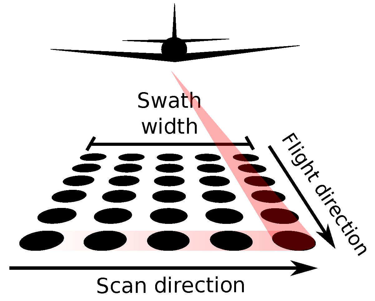
Figure 1. Conceptual illustration of airborne lidar scanning. Scan direction (scan line) is typically perpendicular to the flight direction. The area covered during scanning while an aircraft flies in a constant direction is called the swath or flight strip.
Sensors 23 01593 g001
Figure 2. Scan patterns for basic types of sensors [49,52,53]: (a) line scanner or fiber scanner pattern; (b) rotating polygon or rotating mirror pattern; (c) oscillating or swinging mirror pattern; and (d) conical, elliptical, or Palmer scan pattern.
Sensors 23 01593 g002
Figure 3. Point cloud from several overlapping swaths with an elliptical scan pattern (two swaths in the middle of the stripe of points). Elliptical scanning causes a higher point density at the edge of each swath. Dataset: NOAA/NASA/USGS 1999 [45].
Sensors 23 01593 g003
Figure 4. For some scanners, point density (a) increases towards the end of the scan line and (b) peaks at the very end. The extent of (b) is highlighted in (a). Only points with specific source ID, scan direction, and user data field are displayed to highlight the scan line. Dataset: NC Floodplain Mapping Program 2015 [42].
Sensors 23 01593 g004
Figure 5. Variable aircraft speed and pitch results in areas with higher and lower point density along the flight line (here approximately north-south direction). Point density is expressed as the number of points per grid cell at 6 m resolution (a) and 5 m resolution (b). Darker areas indicate lower point density while lighter areas indicate high density. Datasets: NCALM 2009 [44] (a) and NOAA 2008 [47] (b).
Sensors 23 01593 g005
Figure 6. Example of a complex point distribution. The area is completely covered by one swath and partially covered by another. The border of the second one reveals the doubled scan pattern and higher density at the end of the scan line. There are bands of higher and lower densities in the direction of the flight (approximately diagonal direction). Other density variations are related to vegetation and the small area with missing points on the left is caused by a water body. Dataset: Wake County 2013 [43].
Sensors 23 01593 g006
Figure 7. Swath overlap as the main source of variation in point density. (a) Overlap of two swaths in red and orange around the image diagonal. (b) An abrupt change in the pattern that follows a straight line (close to image diagonal) marks the transition between swaths and removed swath overlap in classified ground points. Additionally, both figures showed a Moiré effect in the point density. Figures show the number of points per grid cell at 1 m resolution. Dataset: Wake County 2013 [43].
Sensors 23 01593 g007
Figure 8. Places with low point density cause differences in skewness of point elevations. (a) Larger area showing two sets of north–south swaths. Color represents the number of points per square meter. (b) Dark violet areas represent places with low point density (<10 points per square meter). (c) Skewness of point elevations. Some areas with zero skewness (in white) are associated with areas with low point density. Most prominent places are marked by red arrows. Skewness is smoothed using circular 23 × 23 moving window to remove local extremes. Dataset: NCALM 2009 [44].
Sensors 23 01593 g008
Figure 9. Error in swath elevation registration (a line close to the image diagonal): (a) Split view between point density and shaded relief (1 meter resolution, year 2013). (b) Elevation difference in meters; year 2015 minus year 2013. (c) Water discharge in m 3 s 1 simulated by SIMWE [65] with default parameters. Datasets: Wake County 2013 [43], NC Floodplain Mapping Program 2015 [42].
Sensors 23 01593 g009
Figure 10. Corduroy effect visible on (a) the interpolated DEM visualized in 3D and (b) the source point cloud (red) overlaid with a DEM-derived skyview factor visualization [71] that shows the low places between corduroy ridges in dark gray. The DEM was interpolated at 0.5 meter resolution. Dataset: NASA/USGS 2003 [46].
Sensors 23 01593 g010
Figure 11. Areas without points caused by (a) a water body and (b) by a dark asphalt roof. Dataset: Wake County 2013 [43].
Sensors 23 01593 g011
Figure 12. Horizontal point pattern in vegetated and nonvegetated areas: (a) Points from all returns had a regular pattern in open areas combined with irregular distributions in the vegetated areas. (b) Classified ground points in areas without vegetation had the original pattern, while in the areas with vegetation the distribution is much sparser. Dataset: NC Floodplain Mapping Program 2015 [42].
Sensors 23 01593 g012
Figure 13. (a) Vertical distribution of lidar points in natural forest (left) and a planted forest (right) in a 220 m long and 30 m wide transect of a forested area. (b) Skewness of point elevations along the same transect without ground points. Dataset: NC Floodplain Mapping Program 2015 [42].
Sensors 23 01593 g013
Figure 14. The blind-zone effect, i.e., no points recorded after a given record, may cause the omission of points in certain parts of the vegetation or on the ground. Emitted pulse penetrates the canopy and produces returns. The first return is from top of the canopy and is registered by a detector. Then, no further returns from the canopy are registered until the detector is ready to record another return (top gray rectangle). When the detector is ready to register again, the second return is recorded from the lower parts of the canopy. Again, no further returns from the canopy or ground are registered because the detector is not ready to record (bottom gray rectangle).
Sensors 23 01593 g014
Figure 15. Lower density of ground points in vegetated areas or lack of points in wet areas usually causes these areas to be smoother than the rest of the area when points are interpolated into a DEM: (a) Lower density of all return points around a stream and in a vegetated, supposedly wet area (marked in blue). (b) Classified ground points (red) missing in some areas completely. The influence on the DEM becomes most apparent when the DEM is used to derive additional products such as the shaded relief here. Dataset: NC Floodplain Mapping Program 2015 [42].
Sensors 23 01593 g015
Figure 16. (a) Point cloud decimated using (b) count-based decimation keeping 1% of points (preserving every 100th point); (c) grid-based decimation preserving one point per 5 meter grid cell; (d) grid-based decimation with snapping to grid using the same 5 meter grid. Dataset: Wake County 2013 [43].
Sensors 23 01593 g016
Table 1. Overview of the six airborne lidar datasets used for demonstrating density variations. All datasets are for parts of North Carolina (NC), USA.
NameYearAreaCollected byReference
NC Floodplain Mapping Program2015Selected counties in PiedmontState of North Carolina[42]
Wake County2013Wake CountyWake County government[43]
NCALM2009Nantahala National ForestNCALM[44]
NOAA/NASA/USGS1999Coast of NCNOAA, NASA, USGS[45]
NASA/USGS2003Cape HatterasNASA, USGS[46]
NOAA2008Coast of NC and VirginiaNOAA[47]
Table 2. Point density variations related to scanner and flight.
Source of Density VariationPossible Effect on Point Density
Scanner typeChange in overall pattern
Variable line scanner point spacingLower or higher density along the scan line
Variable speed or pitchStripes of higher and lower density in the flight direction (banding)
Variable altitudeHigher or lower overall density
Altitude change preventing swath overlapGaps without points
Roll change preventing swath overlapGaps without points
Missing or additional swath due to navigation errorGaps without points or higher point density
Missing or additional swath due to error in flight planningGaps without points or higher point density
Table 3. Errors in interpolated DEM, their relations to density, and their causes.
Cause of DEM ErrorPossible Indication in Density or PatternEffect in DEM
Occlusion, low reflectivityGaps, very low densitySmooth areas (missing information)
Pitch changes and recording errorsDense stripesElevation banding (waves)
Vertically unaligned swathsAbrupt changes in patternAbrupt changes in elevation (break lines)
Vertically unaligned scan linesMoiré effect, double scan linesCorduroy effect (stripes)
Disclaimer/Publisher’s Note: The statements, opinions and data contained in all publications are solely those of the individual author(s) and contributor(s) and not of MDPI and/or the editor(s). MDPI and/or the editor(s) disclaim responsibility for any injury to people or property resulting from any ideas, methods, instructions or products referred to in the content.