
A Multi-Scale Recursive Attention Feature Fusion Network for Image Super-Resolution Reconstruction Algorithm

Abstract
:1. Introduction
- (1)
- An MSRAFFN is proposed that utilizes a multi-scale recursive network structure and attention mechanism to govern network information exchange and effectively handle feature information at different scales.
- (2)
- An MSFE block is proposed to extract feature information from different levels in the form of parallel branch stacked connections, then fuse features between each level layer-by-layer to obtain a reconstructed image with richer texture information.
- (3)
- The AFF block is designed to integrate feature information from each branch within the MSRAFFB and learn the importance of the weights of the features of different branches using the attention mechanism.
- (4)
- The proposed network directly extracts feature information from the LR image without interpolation, uses local residuals to connect neighboring layers within the MSRAFFB to facilitate information transfer within a single block, and utilizes recursion and global residuals to facilitate information exchange between blocks.
2. Related Work
2.1. CNN-Based Super-Resolution of Single Images
2.2. Multi-Scale Networks
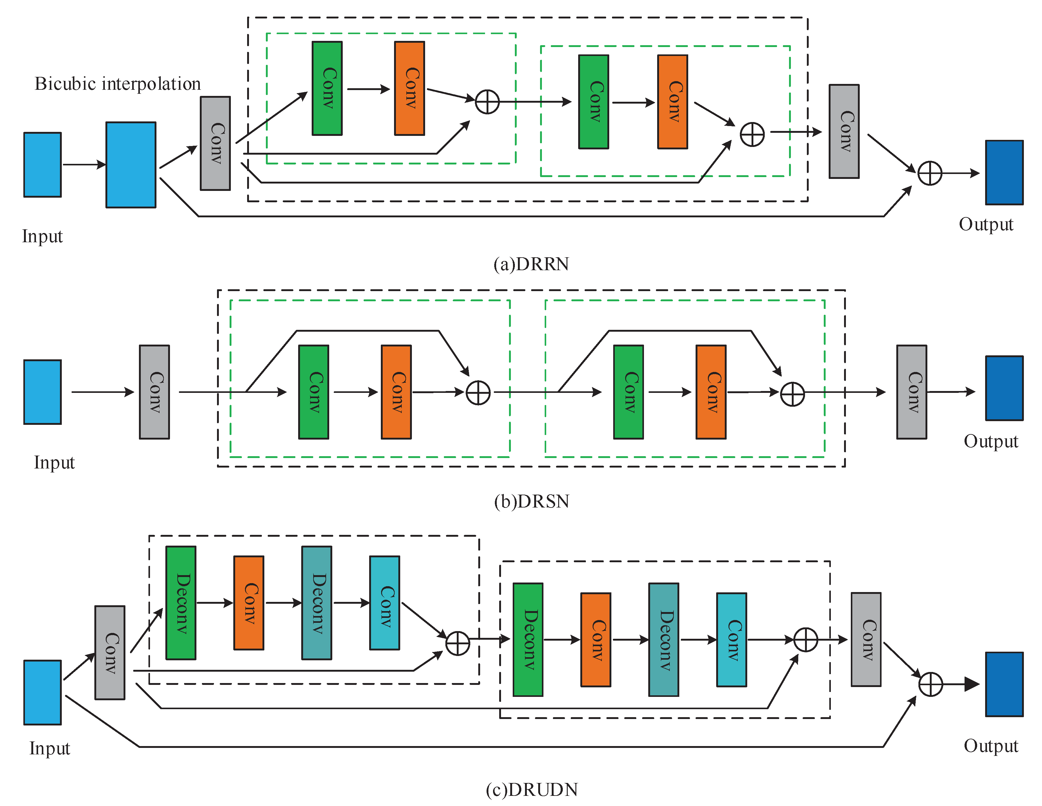
2.3. Recursive-Based SISR Method
2.4. Attention Mechanism
3. Proposed Method
3.1. Overview of the Network Model
3.2. Shallow Feature Extraction Module
3.3. Multi-Scale Recursive Attention Feature Fusion Module
3.4. Reconstruction Module
3.5. Loss Function
4. Experimental Results and Analysis
4.1. Experiment Details
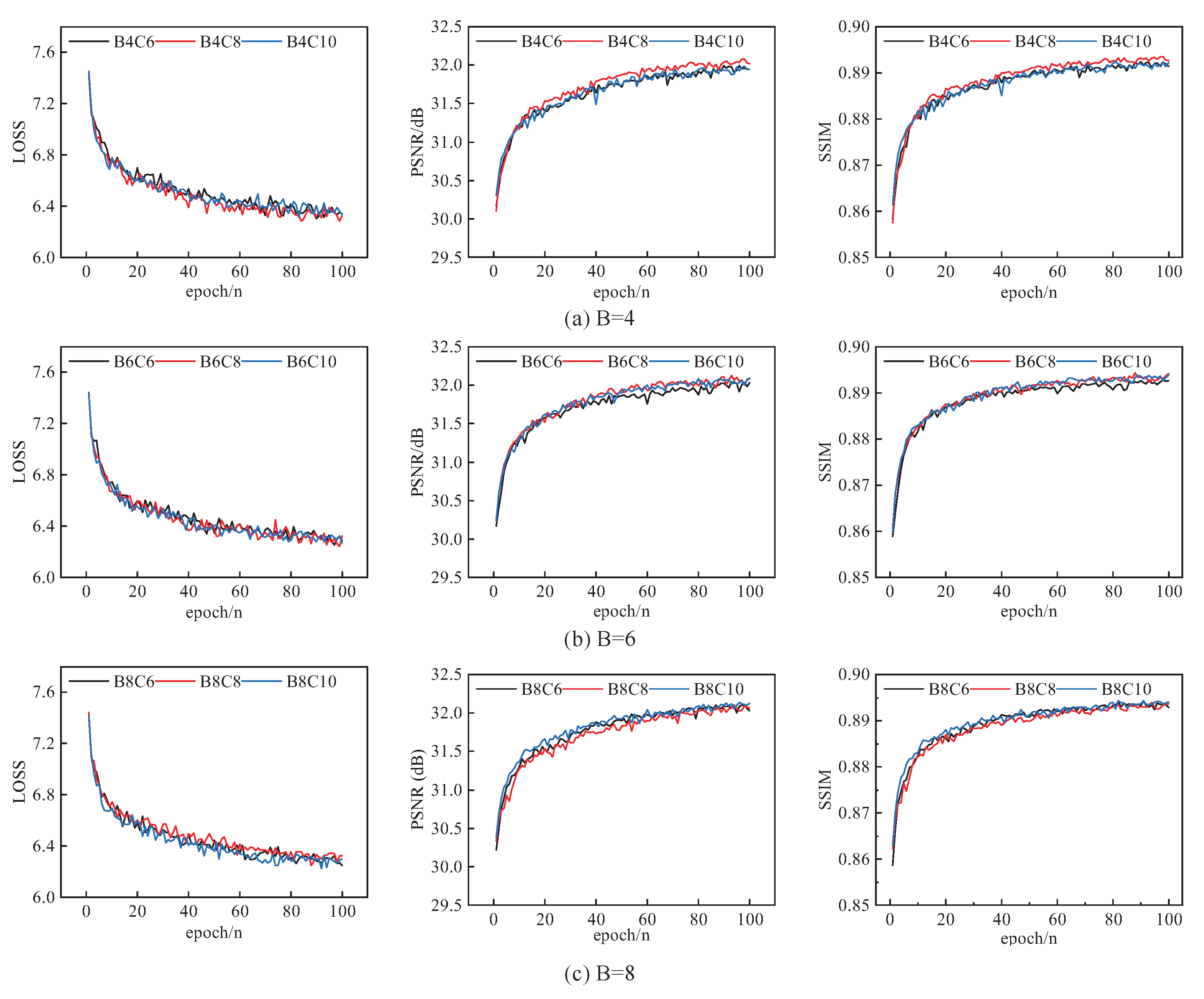
4.2. Network Model Parameters Analysis
4.3. Comparison with State-of-the-Art Methods
4.4. Ablation Study
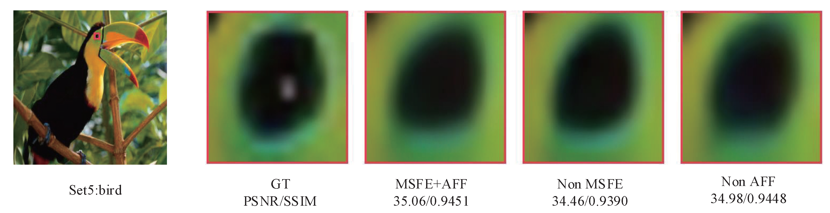
- (1)
- Normal convolution replacing the corresponding MSFE module, denoted as Non MSFE.
- (2)
- A 3 × 3 standard convolution replacing the corresponding AFF module, denoted as Non-AFF.
- (3)
- Both the MSFE and AFF modules are present, denoted as MSFE + AFF.
4.5. Model Performance Analysis
5. Conclusions and Future Prospects
Author Contributions
Funding
Institutional Review Board Statement
Informed Consent Statement
Data Availability Statement
Conflicts of Interest
References
- Anwar, S.; Khan, S.; Barnes, N. A deep journey into super-resolution: A survey. ACM Comput. Surv. (CSUR) 2020, 53, 1–34. [Google Scholar] [CrossRef]
- Wang, Z.; Chen, J.; Hoi, S.C. Deep learning for image super-resolution: A survey. IEEE Trans. Pattern Anal. Mach. Intell. 2020, 43, 3365–3387. [Google Scholar] [CrossRef] [PubMed]
- Bai, Y.; Zhang, Y.; Ding, M.; Ghanem, B. Sod-mtgan: Small object detection via multi-task generative adversarial network. In Proceedings of the European Conference On Computer Vision (ECCV), Munich, Germany, 8–14 September 2018; pp. 206–221. [Google Scholar]
- Bing, X.; Zhang, W.; Zheng, L.; Zhang, Y. Medical image super resolution using improved generative adversarial networks. IEEE Access 2019, 7, 145030–145038. [Google Scholar] [CrossRef]
- Isaac, J.S.; Kulkarni, R. Super resolution techniques for medical image processing. In Proceedings of the 2015 International Conference on Technologies for Sustainable Development (ICTSD), Mumbai, India, 4–6 February 2015; IEEE: Piscataway, NJ, USA, 2015; pp. 1–6. [Google Scholar]
- Sajjadi, M.S.; Vemulapalli, R.; Brown, M. Frame-recurrent video super-resolution. In Proceedings of the IEEE Conference on Computer Vision and Pattern Recognition, Salt Lake City, UT, USA, 18–23 June 2018; pp. 6626–6634. [Google Scholar]
- Shamsolmoali, P.; Zareapoor, M.; Jain, D.K.; Jain, V.K.; Yang, J. Deep convolution network for surveillance records super-resolution. Multimed. Tools Appl. 2019, 78, 23815–23829. [Google Scholar] [CrossRef]
- Dong, R.; Zhang, L.; Fu, H. RRSGAN: Reference-based super-resolution for remote sensing image. IEEE Trans. Geosci. Remote Sens. 2021, 60, 1–17. [Google Scholar] [CrossRef]
- Shabairou, N.; Cohen, E.; Wagner, O.; Malka, D.; Zalevsky, Z. Color image identification and reconstruction using artificial neural networks on multimode fiber images: Towards an all-optical design. Opt. Lett. 2018, 43, 5603–5606. [Google Scholar] [CrossRef] [PubMed]
- Malka, D.; Berke, B.; Tischler, Y.; Zalevsky, Z. Improving Raman spectra of pure silicon using super-resolved method. J. Opt. 2019, 21, 075801. [Google Scholar] [CrossRef]
- Zhao, J.; Chen, C.; Zhou, Z.; Cao, F. Single image super-resolution based on adaptive convolutional sparse coding and convolutional neural networks. J. Vis. Commun. Image Represent. 2019, 58, 651–661. [Google Scholar] [CrossRef]
- Cao, F.; Cai, M.; Tan, Y. Image interpolation via low-rank matrix completion and recovery. IEEE Trans. Circuits Syst. Video Technol. 2014, 25, 1261–1270. [Google Scholar]
- Xu, H.; Zhai, G.; Yang, X. Single image super-resolution with detail enhancement based on local fractal analysis of gradient. IEEE Trans. Circuits Syst. Video Technol. 2013, 23, 1740–1754. [Google Scholar] [CrossRef]
- Arsalan Bashir, S.M.; Wang, Y.; Khan, M.; Niu, Y. A Comprehensive Review of Deep Learning-based Single Image Super-resolution. arXiv 2021, arXiv:2102.09351. [Google Scholar]
- He, K.; Zhang, X.; Ren, S.; Sun, J. Deep residual learning for image recognition. In Proceedings of the IEEE Conference on Computer Vision and Pattern Recognition, Las Vegas, NV, USA, 26 June–1 July 2016; pp. 770–778. [Google Scholar]
- Dong, C.; Loy, C.C.; He, K.; Tang, X. Learning a deep convolutional network for image super-resolution. In Proceedings of the Computer Vision–ECCV 2014: 13th European Conference, Zurich, Switzerland, 6–12 September 2014; Proceedings, Part IV 13. Springer: Berlin/Heidelberg, Germany, 2014; pp. 184–199. [Google Scholar]
- Zhang, Y.; Li, K.; Li, K.; Wang, L.; Zhong, B.; Fu, Y. Image super-resolution using very deep residual channel attention networks. In Proceedings of the European Conference on Computer Vision (ECCV), Munich, Germany, 8–14 September 2018; pp. 286–301. [Google Scholar]
- Hui, Z.; Wang, X.; Gao, X. Fast and accurate single image super-resolution via information distillation network. In Proceedings of the IEEE Conference on Computer Vision and Pattern Recognition, Salt Lake City, UT, USA, 18–23 June 2018; pp. 723–731. [Google Scholar]
- Han, W.; Chang, S.; Liu, D.; Yu, M.; Witbrock, M.; Huang, T.S. Image super-resolution via dual-state recurrent networks. In Proceedings of the IEEE Conference on Computer Vision and Pattern Recognition, Salt Lake City, UT, USA, 18–23 June 2018; pp. 1654–1663. [Google Scholar]
- Dong, C.; Loy, C.C.; Tang, X. Accelerating the super-resolution convolutional neural network. In Proceedings of the Computer Vision–ECCV 2016: 14th European Conference, Amsterdam, The Netherlands, 11–14 October 2016; Proceedings, Part II 14. Springer: Berlin/Heidelberg, Germany, 2016; pp. 391–407. [Google Scholar]
- Simonyan, K.; Zisserman, A. Very deep convolutional networks for large-scale image recognition. arXiv 2014, arXiv:1409.1556. [Google Scholar]
- Shi, W.; Caballero, J.; Huszár, F.; Totz, J.; Aitken, A.P.; Bishop, R.; Rueckert, D.; Wang, Z. Real-time single image and video super-resolution using an efficient sub-pixel convolutional neural network. In Proceedings of the IEEE Conference on Computer Vision and Pattern Recognition, Las Vegas, NV, USA, 26 June–1 July 2016; pp. 1874–1883. [Google Scholar]
- Lai, W.S.; Huang, J.B.; Ahuja, N.; Yang, M.H. Deep laplacian pyramid networks for fast and accurate super-resolution. In Proceedings of the IEEE Conference on Computer Vision and Pattern Recognition, Honolulu, HI, USA, 21–26 July 2017; pp. 624–632. [Google Scholar]
- Hu, Y.; Gao, X.; Li, J.; Huang, Y.; Wang, H. Single image super-resolution via cascaded multi-scale cross network. arXiv 2018, arXiv:1802.08808. [Google Scholar]
- Li, J.; Fang, F.; Mei, K.; Zhang, G. Multi-scale residual network for image super-resolution. In Proceedings of the European Conference on Computer Vision (ECCV), Munich, Germany, 8–14 September 2018; pp. 517–532. [Google Scholar]
- Kim, J.; Lee, J.K.; Lee, K.M. Deeply-recursive convolutional network for image super-resolution. In Proceedings of the IEEE Conference on Computer Vision and Pattern Recognition, Las Vegas, NV, USA, 26 June–1 July 2016; pp. 1637–1645. [Google Scholar]
- Tai, Y.; Yang, J.; Liu, X. Image super-resolution via deep recursive residual network. In Proceedings of the IEEE Conference on Computer Vision and Pattern Recognition, Honolulu, HI, USA, 21–26 July 2017; pp. 3147–3155. [Google Scholar]
- Li, Z.; Li, Q.; Wu, W.; Yang, J.; Li, Z.; Yang, X. Deep recursive up-down sampling networks for single image super-resolution. Neurocomputing 2020, 398, 377–388. [Google Scholar] [CrossRef]
- Shocher, A.; Cohen, N.; Irani, M. “zero-shot” super-resolution using deep internal learning. In Proceedings of the IEEE Conference on Computer Vision and Pattern Recognition, Salt Lake City, UT, USA, 18–23 June 2018; pp. 3118–3126. [Google Scholar]
- Qin, J.; Huang, Y.; Wen, W. Multi-scale feature fusion residual network for single image super-resolution. Neurocomputing 2020, 379, 334–342. [Google Scholar] [CrossRef]
- Ha, V.K.; Ren, J.; Xu, X.; Zhao, S.; Xie, G.; Vargas, V.M. Deep learning based single image super-resolution: A survey. In Proceedings of the Advances in Brain Inspired Cognitive Systems: 9th International Conference, BICS 2018, Xi’an, China, 7–8 July 2018; Proceedings 9. Springer: Berlin/Heidelberg, Germany, 2018; pp. 106–119. [Google Scholar]
- Hu, J.; Shen, L.; Sun, G. Squeeze-and-excitation networks. In Proceedings of the IEEE Conference on Computer Vision and Pattern Recognition, Salt Lake City, UT, USA, 18–23 June 2018; pp. 7132–7141. [Google Scholar]
- Woo, S.; Park, J.; Lee, J.; Kweon, I. Cbam: Convolutional block attention module. In Proceedings of the European Conference On Computer Vision (ECCV), Munich, Germany, 8–14 September 2018; pp. 3–19. [Google Scholar]
- Niu, B.; Wen, W.; Ren, W.; Zhang, X.; Yang, L.; Wang, S.; Zhang, K.; Cao, X.; Shen, H. Single image super-resolution via a holistic attention network. In Proceedings of the Computer Vision—ECCV 2020: 16th European Conference, Glasgow, UK, 23–28 August 2020; Proceedings, Part XII 16. Springer: Berlin/Heidelberg, Germany, 2020; pp. 191–207. [Google Scholar]
- Wu, H.; Zou, Z.; Gui, J.; Zeng, W.; Ye, J.; Zhang, J.; Liu, H.; Wei, Z. Multi-grained attention networks for single image super-resolution. IEEE Trans. Circuits Syst. Video Technol. 2020, 31, 512–522. [Google Scholar] [CrossRef]
- Wang, Z.; Bovik, A.C. A universal image quality index. IEEE Signal Process. Lett. 2002, 9, 81–84. [Google Scholar] [CrossRef]
- Wang, Z.; Bovik, A.C.; Sheikh, H.R.; Simoncelli, E.P. Image quality assessment: From error visibility to structural similarity. IEEE Trans. Image Process. 2004, 13, 600–612. [Google Scholar] [CrossRef] [PubMed]
- Agustsson, E.; Timofte, R. Ntire 2017 challenge on single image super-resolution: Dataset and study. In Proceedings of the IEEE Conference on Computer Vision and Pattern Recognition Workshops, Honolulu, HI, USA, 21–26 July 2017; pp. 126–135. [Google Scholar]
- Kingma, D.P.; Ba, J. Adam: A method for stochastic optimization. arXiv 2014, arXiv:1412.6980. [Google Scholar]
- Bevilacqua, M.; Roumy, A.; Guillemot, C.; Alberi-Morel, M.L. Low-complexity single-image super-resolution based on nonnegative neighbor embedding. In Proceedings of the British Machine Vision Conference, Surrey, UK; 2012; pp. 3–7. [Google Scholar]
- Zeyde, R.; Elad, M.; Protter, M. On single image scale-up using sparse-representations. In Proceedings of the Curves and Surfaces: 7th International Conference, Avignon, France, 24–30 June 2010; Revised Selected Papers 7. Springer: Berlin/Heidelberg, Germany, 2012; pp. 711–730. [Google Scholar]
- Martin, D.; Fowlkes, C.; Tal, D.; Malik, J. A database of human segmented natural images and its application to evaluating segmentation algorithms and measuring ecological statistics. In Proceedings of the Eighth IEEE International Conference on Computer Vision, ICCV 2001, Vancouver, BC, Canada, 7–14 July 2001; IEEE: Piscataway, NJ, USA, 2001; Volume 2, pp. 416–423. [Google Scholar]
- Huang, J.B.; Singh, A.; Ahuja, N. Single image super-resolution from transformed self-exemplars. In Proceedings of the IEEE Conference on Computer Vision and Pattern Recognition, Boston, MA, USA, 7–12 June 2015; pp. 5197–5206. [Google Scholar]
- Matsui, Y.; Ito, K.; Aramaki, Y.; Fujimoto, A.; Ogawa, T.; Yamasaki, T.; Aizawa, K. Sketch-based manga retrieval using manga109 dataset. Multimed. Tools Appl. 2017, 76, 21811–21838. [Google Scholar] [CrossRef]


| Layer | Kernel Size |
|---|---|
| Shallow feature extraction module | 3 × 3 × 64, 3 × 3 × 64 |
| Multi-scale feature extraction unit | 3 × 3 × 64, 3 × 3 × 64, 1 × 1 × 128 |
| 3 × 3 × 64, 1 × 1 × 128, 3 × 3 × 64, 1 × 1 × 128 | |
| 3 × 3 × 64, 1 × 1 × 128, 3 × 3 × 64, 1 × 1 × 128 | |
| 3 × 3 × 64, 1 × 1 × 128, 3 × 3 × 64, 1 × 1 × 128 | |
| Attention feature fusion unit | 1 × 1 × 512 |
| Average_pool, fc1, fc2 | |
| 3 × 3 × 64 | |
| 1 × 1 × 128 | |
| Reconstruction module | 3 × 3 × 64 |
| Deconvolution | |
| 3 × 3 × 64 × 3 |
| Different Methods | Set5 | Set14 | B100 | Urban100 | Manga109 |
|---|---|---|---|---|---|
| PSNR/SSIM | PSNR/SSIM | PSNR/SSIM | PSNR/SSIM | PSNR/SSIM | |
| B4C6 | 31.99/0.8924 | 28.43/0.7777 | 27.45/0.7322 | 25.74/0.7747 | 30.03/0.9029 |
| B4C8 | 32.08/0.8936 | 28.48/0.7790 | 27.48/0.7331 | 25.83/0.7779 | 30.12/0.9045 |
| B4C10 | 31.36/0.8890 | 28.26/0.7747 | 27.33/0.7284 | 25.57/0.7693 | 29.41/0.8962 |
| B6C6 | 32.05/0.8926 | 28.49/0.7781 | 27.49/0.7322 | 25.82/0.7758 | 30.08/0.9036 |
| B6C8 | 32.28/0.8954 | 28.66/0.7828 | 27.61/0.7368 | 26.23/0.7895 | 30.96/0.9108 |
| B6C10 | 32.12/0.8939 | 28.48/0.7795 | 27.48/0.7338 | 25.84/0.7785 | 30.18/0.9050 |
| B8C6 | 32.10/0.8943 | 28.53/0.7795 | 27.50/0.7332 | 25.86/0.7782 | 30.24/0.9061 |
| B8C8 | 32.09/0.8939 | 28.47/0.7791 | 27.50/0.7333 | 25.85/0.7780 | 30.13/0.9045 |
| B8C10 | 31.74/0.8894 | 28.34/0.7768 | 27.37/0.7298 | 25.54/0.7762 | 30.18/0.9050 |
| Methods | Upsampling Methods | Recursive Network | Residual Network | Loss Function |
|---|---|---|---|---|
| SRCNN | bicubic | |||
| FSRCNN | deconvolution | √ | ||
| VDSR | bicubic | √ | MSE | |
| DRCN | bicubic | √ | √ | |
| LapSRN | deconvolution | √ | Char | |
| IDN | deconvolution | √ | MSE | |
| MSRN | subpixel convolution | √ | ||
| Ours | deconvolution | √ | √ |
| Method | Scale | Set5 | Set14 | B100 | Urban100 | Manga109 |
|---|---|---|---|---|---|---|
| PSNR/SSIM | PSNR/SSIM | PSNR/SSIM | PSNR/SSIM | PSNR/SSIM | ||
| Bicubic | 33.66/0.9299 | 30.24/0.8668 | 29.56/0.8431 | 26.88/0.8403 | 30.80/0.9339 | |
| SRCNN [16] | 36.66/0.9542 | 32.45/0.9067 | 31.36/0.8879 | 29.50/0.8946 | 35.60/0.9663 | |
| FSRCNN [20] | 37.00/0.9558 | 32.63/0.9088 | 31.53/0.8920 | 29.88/0.9020 | 36.67/0.9710 | |
| VDSR [21] | 37.53/0.9587 | 33.03/0.9124 | 31.90/0.8960 | 30.76/0.9140 | 37.22/0.9750 | |
| DRCN [26] | 37.63/0.9588 | 33.04/0.9118 | 31.85/0.8942 | 30.75/0.9133 | 37.55/0.9732 | |
| LapSRN [23] | × 2 | 37.52/0.9591 | 32.99/0.9124 | 31.80/0.8949 | 30.41/0.9101 | 37.53/0.9740 |
| DRRN [27] | 37.74/0.9591 | 33.23/0.9136 | 32.05/0.8973 | 31.23/0.9188 | 37.88/0.9749 | |
| DSRN [19] | 37.66/0.9590 | 33.15/0.9130 | 32.10/0.8970 | 30.97/0.9160 | -/- | |
| IDN [18] | 37.83/0.9600 | 33.30/0.9148 | 32.08/0.8985 | 31.27/0.9196 | -/- | |
| MSRN [25] | 38.08/0.9605 | 33.74/0.9170 | 32.23/0.9013 | 32.22/0.9326 | 38.82/0.9868 | |
| Proposed Method | 38.03/0.9607 | 33.58/0.9178 | 32.18/0.8998 | 32.22/0.9289 | 38.83/0.9776 | |
| Bicubic | 30.39/0.8682 | 27.55/0.7742 | 27.21/0.7385 | 24.46/0.7349 | 26.95/0.8556 | |
| SRCNN [16] | 32.75/0.9090 | 29.30/0.8215 | 28.41/0.7863 | 26.24/0.7989 | 30.48/0.9117 | |
| FSRCNN [20] | 33.18/0.9140 | 29.37/0.8240 | 28.53/0.7910 | 26.43/0.8080 | 31.10/0.9210 | |
| VDSR [21] | 33.66/0.9213 | 29.77/0.8314 | 28.82/0.7976 | 27.14/0.8279 | 32.01/0.9340 | |
| DRCN [26] | 33.82/0.9226 | 29.76/0.8311 | 28.80/0.7963 | 27.15/0.8276 | 32.24/0.9343 | |
| LapSRN [23] | × 3 | 33.82/0.9227 | 29.79/0.8320 | 28.82/0.7973 | 27.07/0.8271 | 32.21/0.9350 |
| DRRN [27] | 34.03/0.9244 | 29.96/0.8349 | 28.95/0.8004 | 27.53/0.8375 | 32.71/0.9379 | |
| DSRN [19] | 33.88/0.9220 | 30.26/0.8370 | 28.81/0.7970 | 27.16/0.8280 | -/- | |
| IDN [18] | 34.11/0.9253 | 29.99/0.8354 | 28.95/0.8013 | 27.42/0.8359 | -/- | |
| MSRN [25] | 34.38/0.9262 | 30.34/0.8395 | 29.08/0.8041 | 28.08/0.8554 | 33.44/0.9427 | |
| Proposed Method | 34.48/0.9282 | 30.35/0.8421 | 29.11/0.8059 | 28.27/0.8543 | 33.81/0.9460 | |
| Bicubic | 28.42/0.8104 | 26.00/0.7027 | 25.96/0.6675 | 23.14/0.6577 | 24.89/0.7866 | |
| SRCNN [16] | 30.48/0.8628 | 27.50/0.7513 | 26.90/0.7101 | 24.52/0.7221 | 27.58/0.8555 | |
| FSRCNN [20] | 30.72/0.8660 | 27.61/0.7550 | 26.98/0.7150 | 24.62/0.7280 | 27.90/0.8610 | |
| VDSR [21] | 31.35/0.8838 | 28.01/0.7674 | 27.29/0.7251 | 25.18/0.7524 | 28.83/0.8870 | |
| DRCN [26] | 31.53/0.8854 | 28.02/0.7670 | 27.23/0.7233 | 25.14/0.7510 | 28.93/0.8854 | |
| LapSRN [23] | × 4 | 31.54/0.8866 | 28.09/0.7694 | 27.32/0.7264 | 25.21/0.7553 | 29.09/0.8900 |
| DRRN [27] | 31.68/0.8888 | 28.21/0.7721 | 27.38/0.7284 | 25.44/0.7638 | 29.45/0.8946 | |
| DSRN [19] | 31.40/0.8830 | 28.07/0.7700 | 27.25/0.7240 | 25.08/0.7470 | -/- | |
| IDN [18] | 31.82/0.8903 | 28.25/0.7730 | 27.41/0.7297 | 25.41/0.7632 | -/- | |
| MSRN [25] | 32.07/0.8903 | 28.60/0.7751 | 27.52/0.7273 | 26.04/0.7896 | 30.17/0.9034 | |
| Proposed Method | 32.28/0.8954 | 28.66/0.7828 | 27.61/0.7368 | 26.23/0.7895 | 30.96/0.9108 |
| Method | Set5 | Set14 | B100 | Urban100 | Mnaga109 |
|---|---|---|---|---|---|
| PSNR/SSIM | PSNR/SSIM | PSNR/SSIM | PSNR/SSIM | PSNR/SSIM | |
| MSFE + AFF | 32.28/0.8954 | 28.66/0.7828 | 27.61/0.7368 | 26.23/0.7895 | 30.96/0.9108 |
| Non MSFE | 31.97/0.8918 | 28.40/0.7772 | 27.43/0.7312 | 25.72/0.7732 | 29.90/0.9015 |
| Non AFF | 32.25/0.8960 | 28.63/0.7827 | 27.59/0.7369 | 26.16/0.7886 | 30.55/0.9098 |
Disclaimer/Publisher’s Note: The statements, opinions and data contained in all publications are solely those of the individual author(s) and contributor(s) and not of MDPI and/or the editor(s). MDPI and/or the editor(s) disclaim responsibility for any injury to people or property resulting from any ideas, methods, instructions or products referred to in the content. |
© 2023 by the authors. Licensee MDPI, Basel, Switzerland. This article is an open access article distributed under the terms and conditions of the Creative Commons Attribution (CC BY) license (https://creativecommons.org/licenses/by/4.0/).
Share and Cite
Han, X.; Wang, L.; Wang, X.; Zhang, P.; Xu, H. A Multi-Scale Recursive Attention Feature Fusion Network for Image Super-Resolution Reconstruction Algorithm. Sensors 2023, 23, 9458. https://doi.org/10.3390/s23239458
Han X, Wang L, Wang X, Zhang P, Xu H. A Multi-Scale Recursive Attention Feature Fusion Network for Image Super-Resolution Reconstruction Algorithm. Sensors. 2023; 23(23):9458. https://doi.org/10.3390/s23239458
Chicago/Turabian StyleHan, Xiaowei, Lei Wang, Xiaopeng Wang, Pengchao Zhang, and Haoran Xu. 2023. "A Multi-Scale Recursive Attention Feature Fusion Network for Image Super-Resolution Reconstruction Algorithm" Sensors 23, no. 23: 9458. https://doi.org/10.3390/s23239458
APA StyleHan, X., Wang, L., Wang, X., Zhang, P., & Xu, H. (2023). A Multi-Scale Recursive Attention Feature Fusion Network for Image Super-Resolution Reconstruction Algorithm. Sensors, 23(23), 9458. https://doi.org/10.3390/s23239458