
Visibility Estimation Based on Weakly Supervised Learning under Discrete Label Distribution

Abstract
:1. Introduction
- (1)
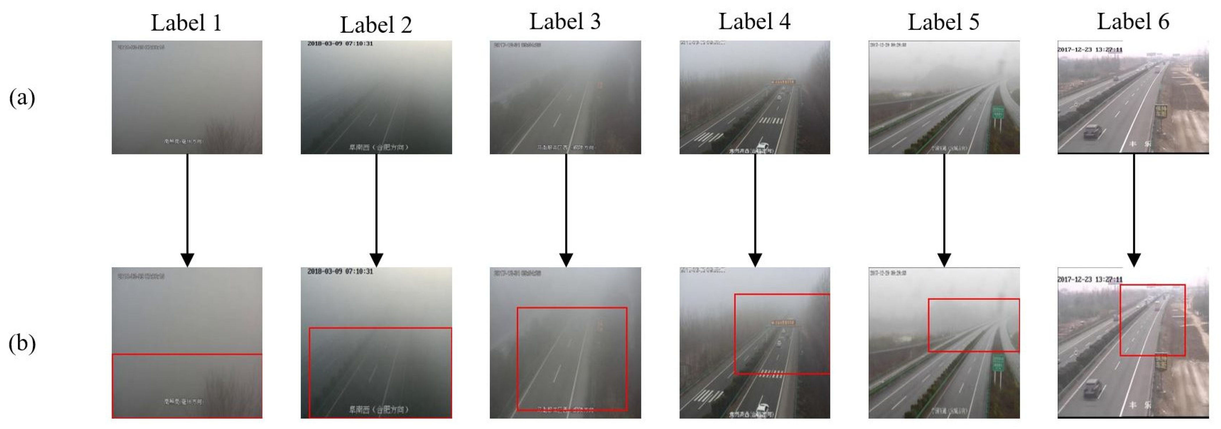
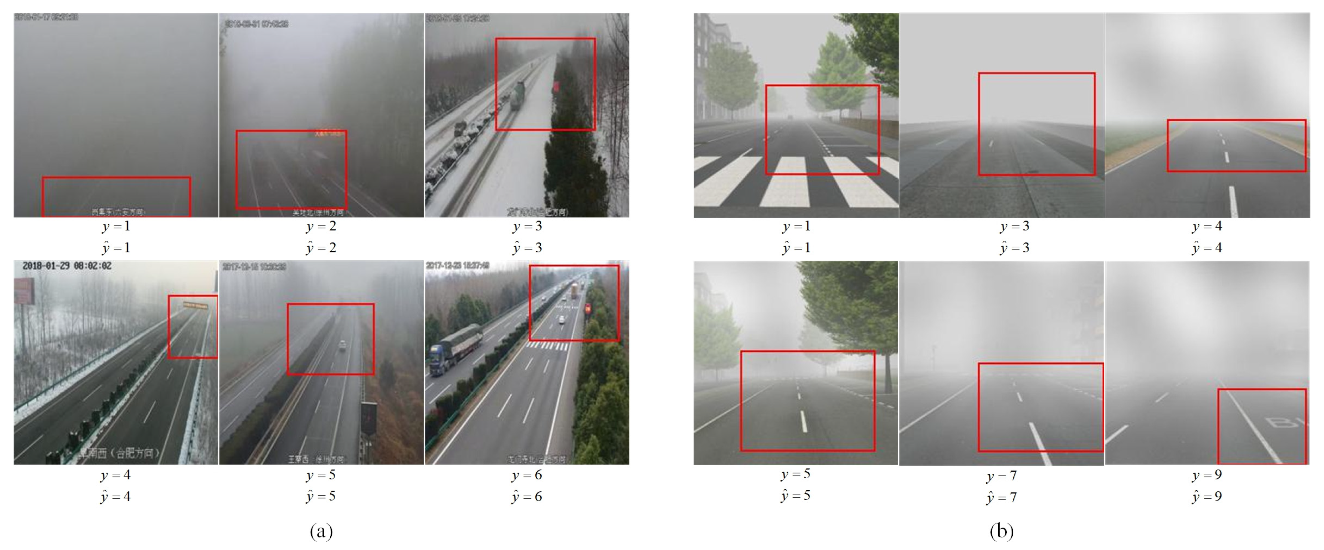
- We propose a weakly supervised localization module to find the farthest visible area in a single image without the need for additional manpower, which is served as auxiliary information to help the network learn to capture fog features.
- (2)
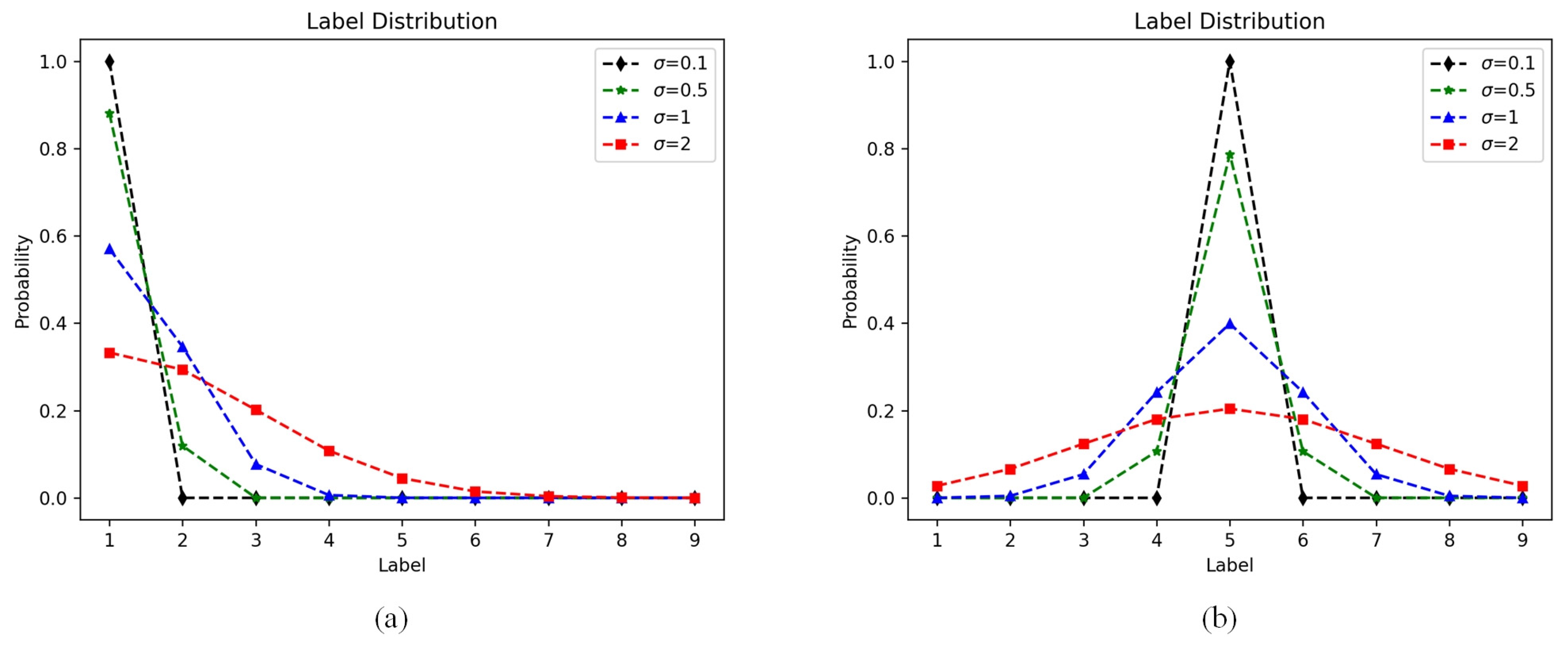
- We propose a discrete label distribution learning module. The fog in foggy images is usually unevenly distributed. By using Gaussian sampling to transform the original fixed classification labels into Gaussian distribution labels, the network can learn this uneven distribution, thus better adapting to the distribution of visibility levels in the image and achieving better results.
2. Related Works
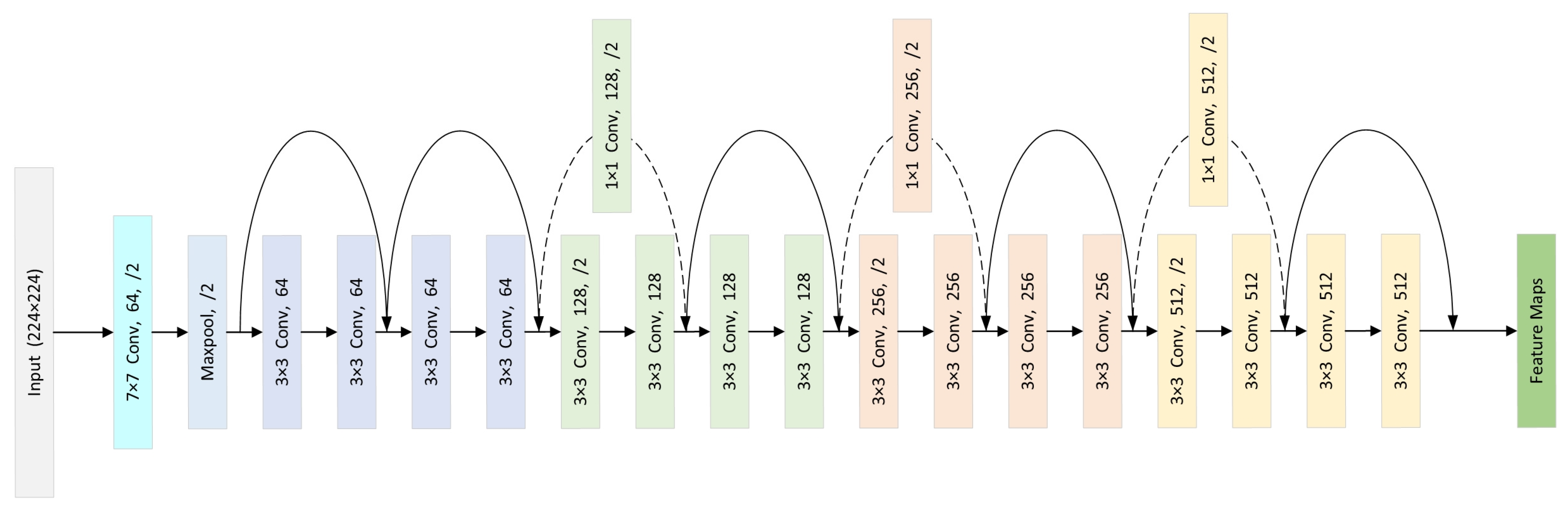
2.1. ResNet
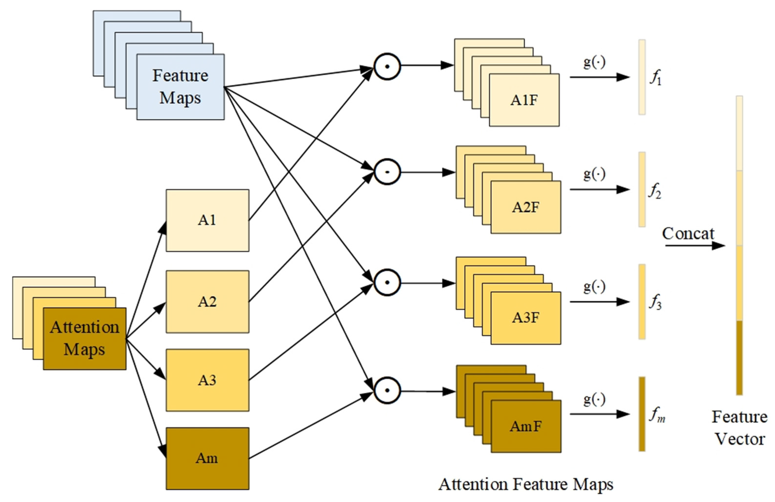
2.2. Bilinear Attention Pooling
2.3. Attention-Guided Location
2.4. Discrete Label Distribution Learning
3. Methods
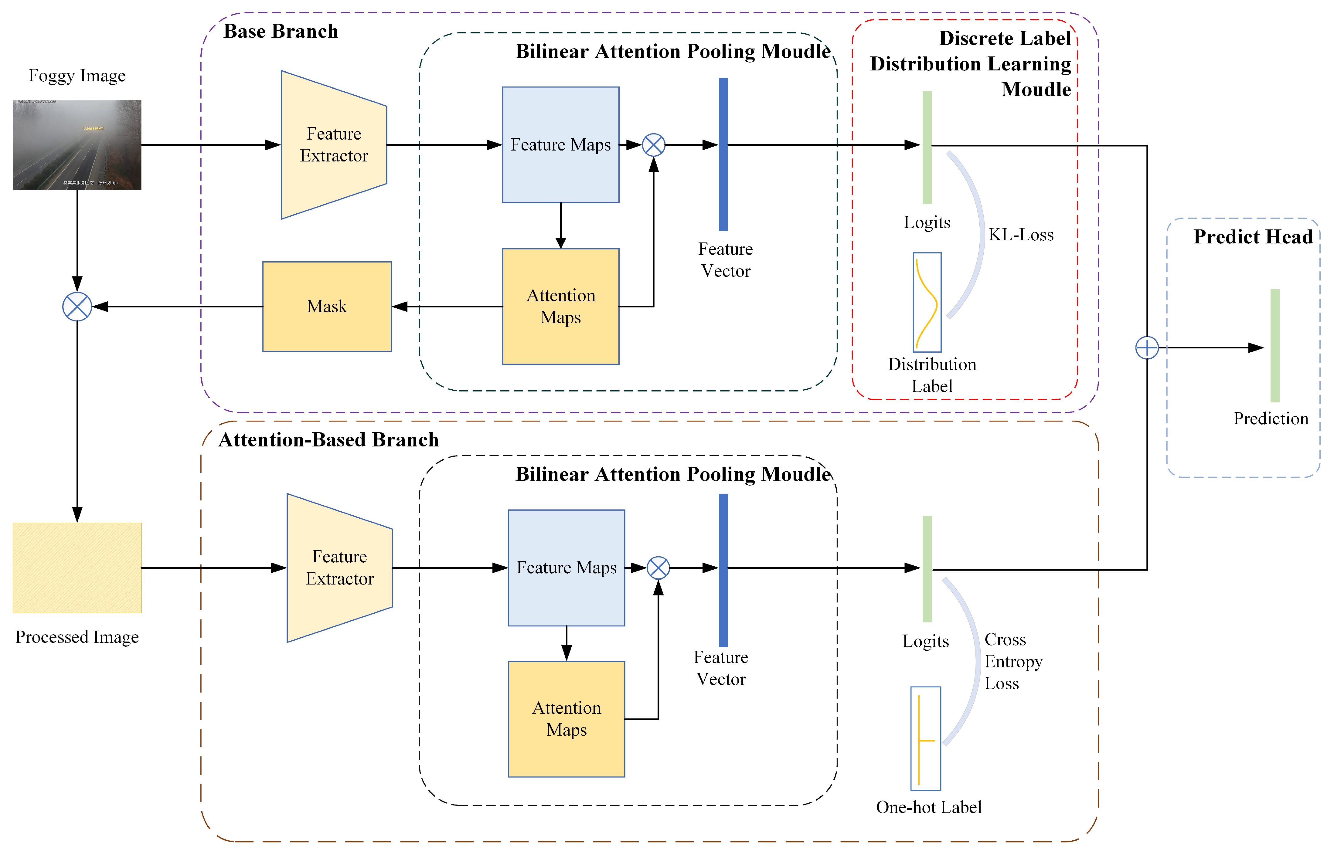
3.1. Overview
3.2. Base Branch
3.3. Attention-Based Branch
3.4. Loss Function
4. Experiment
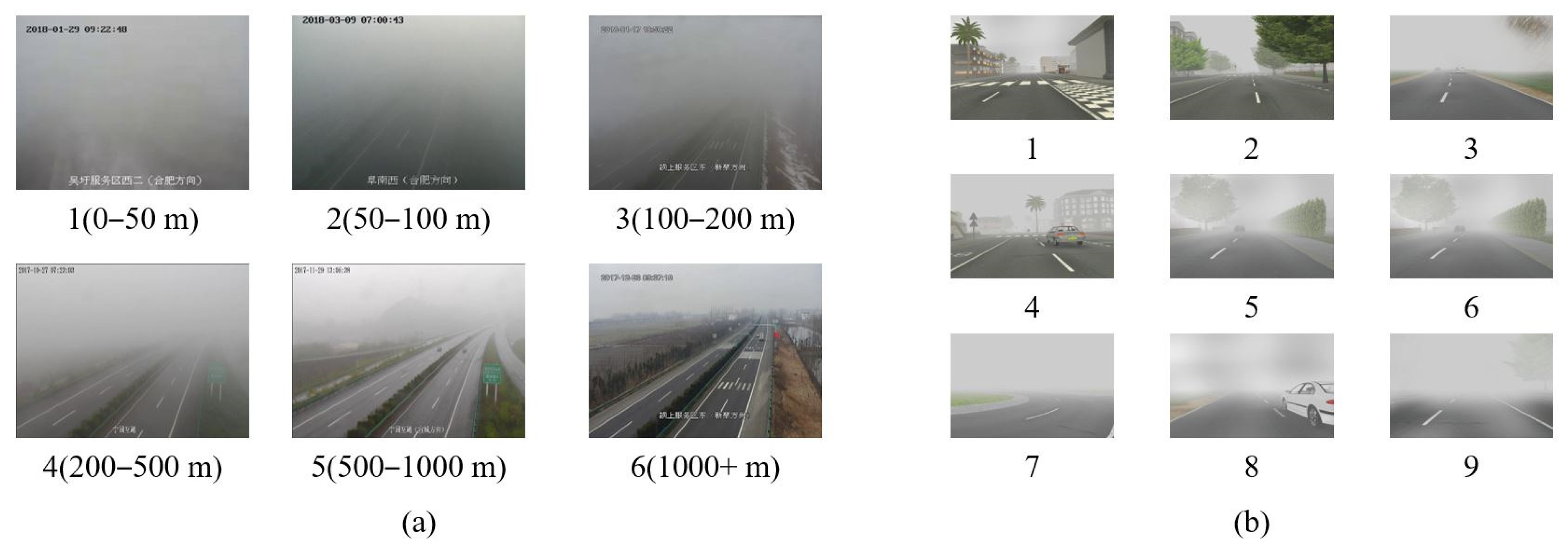
4.1. Dataset
4.1.1. RFID
4.1.2. FRIDA
4.2. Evaluation Index
4.3. Implementation Details
4.4. Experimental Results and Discussions
4.4.1. Hyper-Parameter Settings
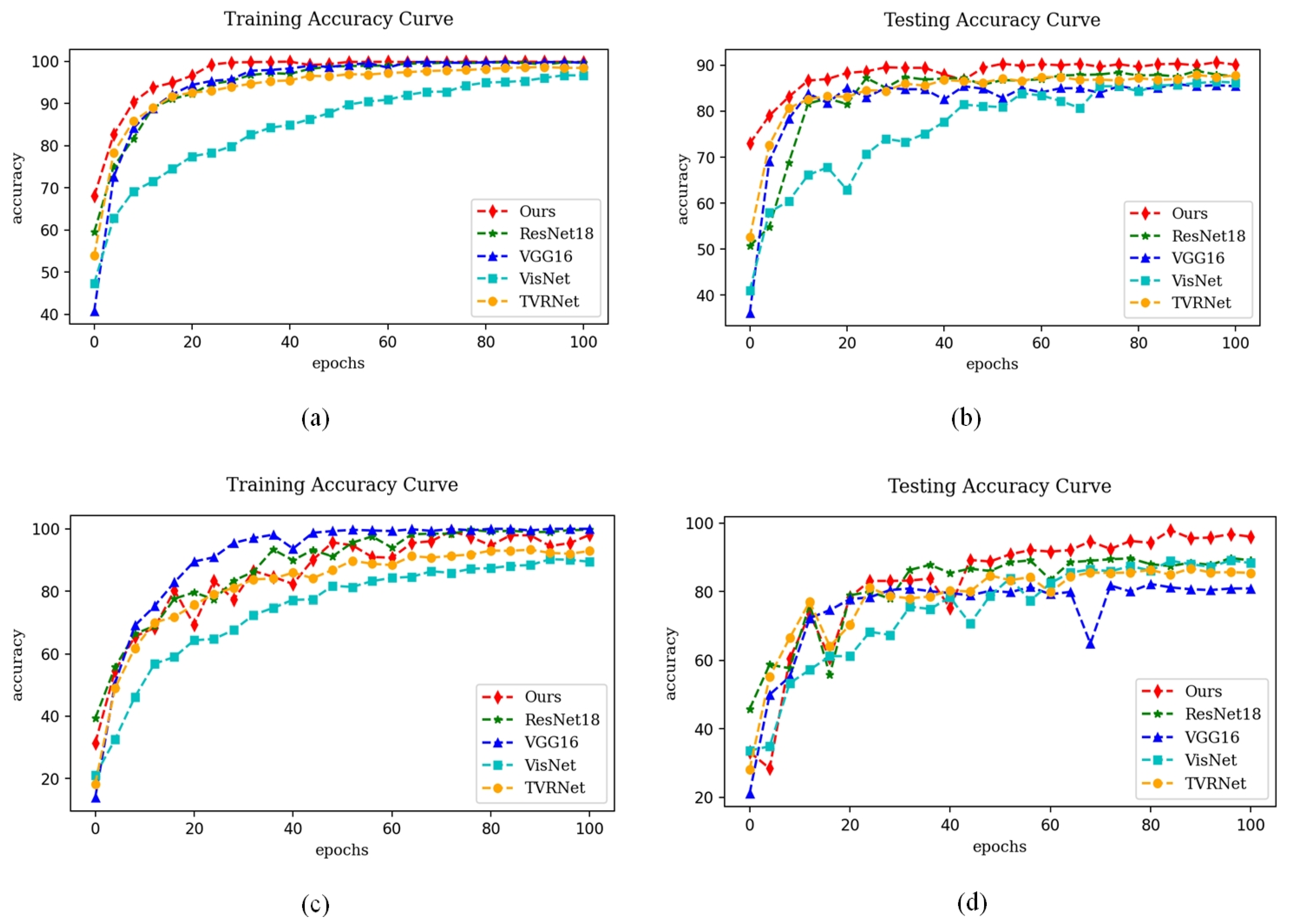
4.4.2. Comparison with State-of-the-Art Methods
4.4.3. Ablation Study
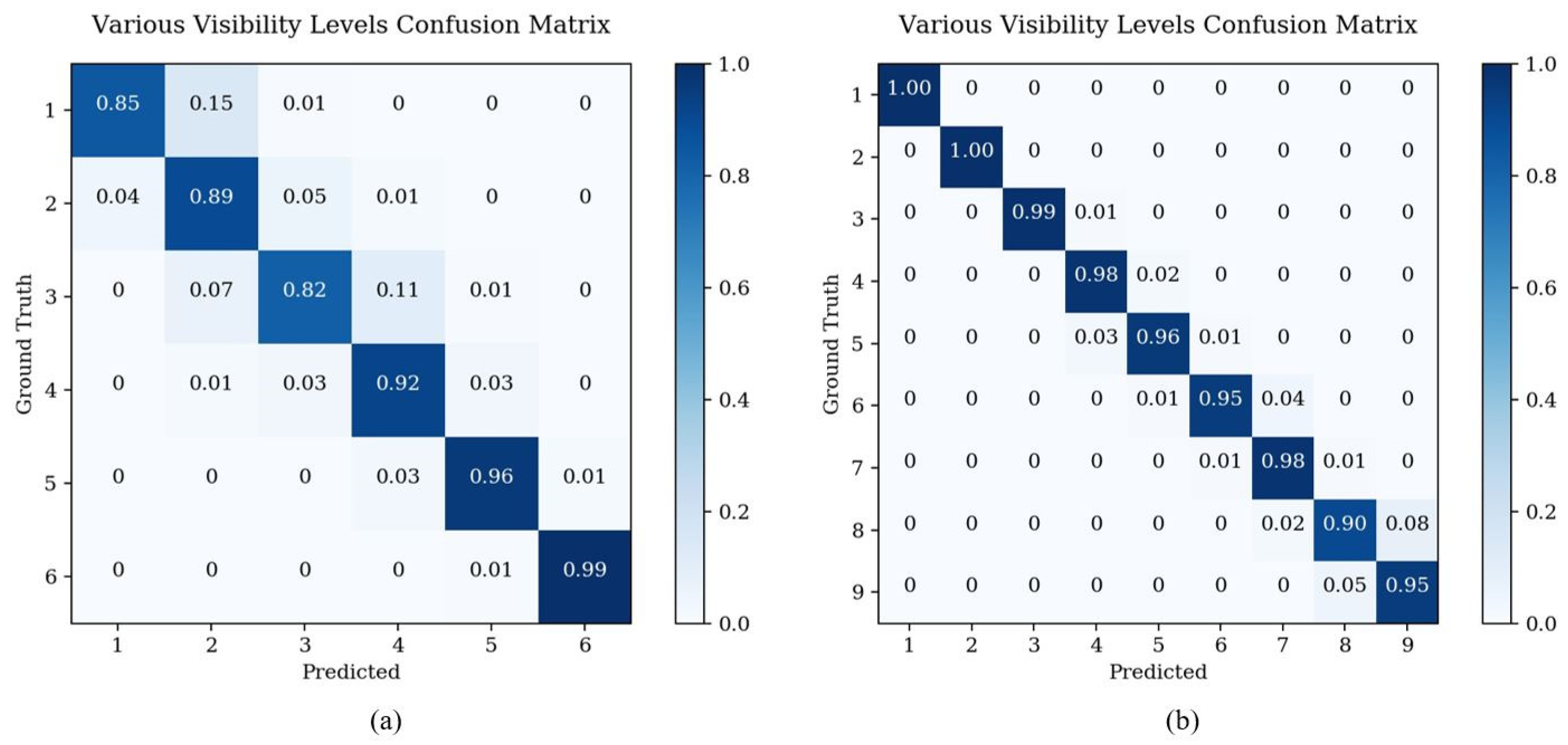
4.4.4. Analysis of Various Visibility Levels
4.4.5. Algorithm Complexity Study
5. Conclusions
Author Contributions
Funding
Institutional Review Board Statement
Informed Consent Statement
Data Availability Statement
Acknowledgments
Conflicts of Interest
References
- World Meteorological Organization (WMO). Guide to Meteorological Instruments and Methods of Observation, 7th ed.; World Meteorological Organization (WMO): Geneva, Switzerland, 1996. [Google Scholar]
- Chinese: Grade of Fog Forecast gb/t 27964¨c2011. Available online: https://openstd.samr.gov.cn/bzgk/gb/newGbInfo?hcno=F0E92BAD8204180AA7AB052A3FD73B70 (accessed on 20 September 2023).
- Tan, R.T. Visibility in bad weather from a single image. In Proceedings of the 2008 IEEE Conference on Computer Vision and Pattern Recognition (CVPR), Anchorage, AK, USA, 23–28 June 2008; pp. 1–8. [Google Scholar]
- Narasimhan, S.G.; Nayar, S.K. Contrast Restoration of Weather Degraded Images. IEEE Trans. Pattern Anal. Mach. Intell. 2003, 25, 713–724. [Google Scholar] [CrossRef]
- Road Traffic Injuries. Available online: https://weather.com/news/news/fog-driving-travel-danger-20121127 (accessed on 20 September 2023).
- Kipfer, K. Fog Prediction with Deep Neural Networks. Master’s Thesis, ETH Zurich, Zurich, Switzerland, 2017. [Google Scholar]
- Krizhevsky, A.; Sutskever, I.; Hinton, G.E. Imagenet Classification with Deep Convolutional Neural Networks. Commun. ACM 2012, 60, 84–90. [Google Scholar] [CrossRef]
- He, K.; Zhang, X.; Ren, S.; Sun, J. Deep Residual Learning for Image Recognition. In Proceedings of the IEEE Conference on Computer Vision and Pattern Recognition (CVPR), Boston, MA, USA, 8–10 June 2015; pp. 770–778. [Google Scholar]
- Simonyan, K.; Zisserman, A. Very Deep Convolutional Networks for Large-Scale Image Recognition. In Proceedings of the Computer Vision and Pattern Recognition (CVPR), Columbus, OH, USA, 23–28 June 2014. [Google Scholar]
- Szegedy, C.; Liu, W.; Jia, Y.Q.; Sermanet, P.; Reed, S.; Anguelov, D.; Erhan, D.; Vanhoucke, V.; Rabinovich, A. Going Deeper with Convolutions. In Proceedings of the IEEE Conference on Computer Vision and Pattern Recognition (CVPR), Boston, MA, USA, 7–12 June 2015; pp. 1–9. [Google Scholar]
- Szegedy, C.; Ioffe, S.; Vanhoucke, V.; Alemi, A.A. Inception-v4, Inception-ResNet and the Impact of Residual Connections on Learning. In Proceedings of the 31st AAAI Conference on Artificial Intelligence, San Francisco, CA, USA, 4–9 February 2017; pp. 4278–4284. [Google Scholar]
- Szegedy, C.; Vanhoucke, V.; Ioffe, S.; Shlens, J.; Wojna, Z. Rethinking the Inception Architecture for Computer Vision. In Proceedings of the IEEE Conference on Computer Vision and Pattern Recognition, Las Vegas, NV, USA, 27–30 June 2016; pp. 2818–2826. [Google Scholar]
- Li, S.; Fu, H.; Lo, W.-L. Meteorological Visibility Evaluation on Webcam Weather Image using Deep Learning Features. Int. J. Comput. Theory Eng 2017, 9, 455–461. [Google Scholar] [CrossRef]
- Zou, X.; Wu, J.; Cao, Z.; Qian, Y.; Zhang, S.; Han, L.; Liu, S.; Zhang, J.; Song, Y. An Atmospheric Visibility Grading Method Based on Ensemble Learning and Stochastic Weight Average. Atmosphere 2021, 12, 869. [Google Scholar] [CrossRef]
- Lo, W.L.; Zhu, M.; Fu, H. Meteorology Visibility Estimation by using Multi-Support Vector Regression Method. J. Adv. Inf. Technol. Vol 2020, 11, 40–47. [Google Scholar] [CrossRef]
- Lo, W.L.; Chung, H.S.H.; Fu, H. Experimental Evaluation of PSO based Transfer Learning Method for Meteorological Visibility Estimation. Atmosphere 2021, 12, 828. [Google Scholar] [CrossRef]
- Li, J.; Lo, W.L.; Fu, H.; Chung, H.S.H. A Transfer Learning Method for Meteorological Visibility Estimation based on Feature Fusion Method. Appl. Sci. 2021, 11, 997. [Google Scholar] [CrossRef]
- You, Y.; Lu, C.; Wang, W.; Tang, C.-K. Relative CNN-RNN: Learning Relative Atmospheric Visibility from Images. IEEE Trans. Image Process. 2018, 28, 45–55. [Google Scholar] [CrossRef]
- Xiao, G.B.; Ma, J.Y.; Wang, S.P.; Chen, C.W. Deterministic Model Fitting by Local-Neighbor Preservation and Global-Residual Optimization. IEEE Trans. Image Process. 2020, 29, 8988–9001. [Google Scholar] [CrossRef]
- Xiao, G.B.; Luo, H.; Zeng, K.; Wei, L.Y.; Ma, J.Y. Robust Feature Matching for Remote Sensing Image Registration via Guided Hyperplane Fitting. IEEE Trans. Geosci. Remote Sens. 2022, 60, 14. [Google Scholar] [CrossRef]
- Hu, J.; Shen, L.; Sun, G. Squeeze-and-Excitation Networks. In Proceedings of the IEEE Conference on Computer Vision and Pattern Recognition (CVPR), Salt Lake City, UT, USA, 18–23 June 2018; pp. 7132–7141. [Google Scholar]
- Woo, S.; Park, J.; Lee, J.-Y.; Kweon, I.S. CBAM: Convolutional Block Attention Module. In Proceedings of the European Conference on Computer Vision (ECCV), Munich, Germany, 8–14 September 2018; pp. 3–19. [Google Scholar]
- Zhao, H.; Kong, X.; He, J.; Qiao, Y.; Dong, C. Efficient Image Super-Resolution using Pixel Attention. In Proceedings of the European Conference on Computer Vision (ECCV), Glasgow, UK, 23–28 August 2020; pp. 56–72. [Google Scholar]
- Hu, T.; Qi, H.; Huang, Q.; Lu, Y. See Better Before Looking Closer: Weakly supervised Data Augmentation Network for Fine-Grained Visual Classification. arXiv 2019, arXiv:1901.09891. [Google Scholar]
- Zhao, W.; Wang, H. Strategic Decision-Making Learning from Label Distributions: An Approach for Facial Age Estimation. Sensors 2016, 16, 994. [Google Scholar] [CrossRef] [PubMed]
- Gao, B.-B.; Liu, X.-X.; Zhou, H.-Y.; Wu, J.; Geng, X. Learning Expectation of Label Distribution for Facial Age and Attractiveness Estimation. arXiv 2020, arXiv:2007.01771. [Google Scholar]
- Gao, B.-B.; Xing, C.; Xie, C.-W.; Wu, J.; Geng, X. Deep Label Distribution Learning with Label Ambiguity. IEEE Trans. Image Process. 2017, 26, 2825–2838. [Google Scholar] [CrossRef] [PubMed]
- Xu, N.; Liu, Y.-P.; Geng, X. Label Enhancement for Label Distribution Learning. IEEE Trans. Knowl. Data Eng. 2019, 33, 1632–1643. [Google Scholar] [CrossRef]
- Geng, X. Label Distribution Learning. IEEE Trans. Knowl. Data Eng. 2016, 28, 1734–1748. [Google Scholar] [CrossRef]
- Chen, S.; Zhang, C.; Dong, M.; Le, J.; Rao, M. Using Ranking-CNN for Age Estimation. In Proceedings of the IEEE Conference on Computer Vision and Pattern Recognition (CVPR), Honolulu, HI, USA, 21–26 July 2017; pp. 5183–5192. [Google Scholar]
- Sakaridis, C.; Dai, D.; Van Gool, L. Semantic Foggy Scene Understanding with Synthetic Data. Int. J. Comput. Vis. 2018, 126, 973–992. [Google Scholar] [CrossRef]
- Lin, T.-Y.; RoyChowdhury, A.; Maji, S. Bilinear CNN Models for Fine-Grained Visual Recognition. In Proceedings of the IEEE International Conference on Computer Vision (ICCV), Santiago, Chile, 11–18 December 2015; pp. 1449–1457. [Google Scholar]
- Xun, L.; Zhang, H.; Yan, Q.; Wu, Q.; Zhang, J. VISOR-NET: Visibility Estimation Based on Deep Ordinal Relative Learning under Discrete-Level Labels. Sensors 2022, 22, 6227. [Google Scholar] [CrossRef]
- Liu, Z.; Chen, Y.; Gu, X.; Yeoh, J.K.; Zhang, Q. Visibility Classification and Influencing-Factors Analysis of Airport: A Deep Learning Approach. Atmos. Environ. 2022, 278, 119085. [Google Scholar] [CrossRef]
- Park, S.; Kwak, N. Analysis on the Dropout Effect in Convolutional Neural Networks. In Proceedings of the 13th Asian Conference on Computer Vision (ACCV), Taipei, Taiwan, 20–24 November 2016; pp. 189–204. [Google Scholar]
- Kumar Singh, K.; Jae Lee, Y. Hide-and-seek: Forcing a Network to be Neticulous for Weakly-Supervised Object and Action Localization. In Proceedings of the IEEE International Conference on Computer Vision (ICCV), Venice, Italy, 22–29 October 2017; pp. 3524–3533. [Google Scholar]
- DeVries, T.; Taylor, G.W. Improved Regularization of Convolutional Neural Networks with Cutout. arXiv 2017, arXiv:1708.04552. [Google Scholar]
- Tarel, J.-P.; Hautiere, N.; Caraffa, L.; Cord, A.; Halmaoui, H.; Gruyer, D. Vision Enhancement in Homogeneous and Heterogeneous Fog. IEEE Intell. Transp. Syst. Mag. 2012, 4, 6–20. [Google Scholar] [CrossRef]
- Li, Y.; Huang, J.; Luo, J. Using User Generated Online Photos to Estimate and Monitor Air Pollution in Major Cities. In Proceedings of the 7th International Conference on Internet Multimedia Computing and Service, Zhangjiajie, China, 19–21 August 2015; pp. 1–5. [Google Scholar]
- Tarel, J.-P.; Hautiere, N.; Cord, A.; Gruyer, D.; Halmaoui, H. Improved Visibility of Road Scene Images under Heterogeneous Fog. In Proceedings of the 2010 IEEE Intelligent Vehicles Symposium, San Diego, CA, USA, 21–24 June 2010; pp. 478–485. [Google Scholar]
- Palvanov, A.; Cho, Y.I. Visnet: Deep Convolutional Neural Networks for Forecasting Atmospheric Visibility. Sensors 2019, 19, 1343. [Google Scholar] [CrossRef]
- Giyenko, A.; Palvanov, A.; Cho, Y. Application of Convolutional Neural Networks for Visibility Estimation of CCTV Images. In Proceedings of the 2018 International Conference on Information Networking (ICOIN), Chiang Mai, Thailand, 10–12 January 2018; pp. 875–879. [Google Scholar]
- Qin, H.; Qin, H. An End-to-End Traffic Visibility Regression Algorithm. IEEE Access 2021, 10, 25448–25454. [Google Scholar] [CrossRef]


| Datasets | 1 | 2 | 3 | 4 | 5 | 6 | 7 | 8 | 9 | Total |
|---|---|---|---|---|---|---|---|---|---|---|
| RFID | 304 | 622 | 774 | 891 | 948 | 1610 | / | / | / | 5149 |
| FRIDA | 336 | 336 | 336 | 336 | 336 | 336 | 336 | 336 | 336 | 3024 |
| Item | Content |
|---|---|
| CPU | Intel Xeon(R) Silver 4214R |
| GPU | RTX 3080Ti |
| RAM | 128 GB |
| Operating System | Ubuntu 20.04.4 LTS |
| Programming Language | Python 3.7.9 |
| Deep Learning Framework | Pytorch 1.7.1 |
| CUDA Version | 11.0 |
| RFID | FRIDA | |||||
|---|---|---|---|---|---|---|
| Accuracy (%) ↑ | RMSE ↓ | F1 ↑ | Accuracy (%) ↑ | RMSE ↓ | F1 ↑ | |
| 1 | 89.67 | 0.3677 | 0.8985 | 92.89 | 0.277 | 0.9288 |
| 2 | 90.22 | 0.3592 | 0.9047 | 93.11 | 0.2541 | 0.9312 |
| 4 | 90.11 | 0.3393 | 0.9020 | 94.78 | 0.2252 | 0.9479 |
| 8 | 90.00 | 0.3382 | 0.9042 | 95.67 | 0.2016 | 0.9565 |
| 16 | 89.78 | 0.3697 | 0.8985 | 96.00 | 0.2024 | 0.9599 |
| 32 | 89.67 | 0.3566 | 0.8972 | 95.11 | 0.2297 | 0.9511 |
| 64 | 89.67 | 0.3404 | 0.8972 | 95.00 | 0.2165 | 0.9500 |
| RFID | FRIDA | |||||
|---|---|---|---|---|---|---|
| Accuracy (%) ↑ | RMSE ↓ | F1 ↑ | Accuracy (%) ↑ | RMSE ↓ | F1 ↑ | |
| 0.1 | 90.00 | 0.3409 | 0.8969 | 95.22 | 0.2197 | 0.9518 |
| 0.2 | 90.22 | 0.3409 | 0.9026 | 96.11 | 0.1954 | 0.9611 |
| 0.5 | 89.67 | 0.3647 | 0.8962 | 94.22 | 0.2327 | 0.9421 |
| 1 | 88.78 | 0.3983 | 0.8885 | 94.22 | 0.2364 | 0.9425 |
| 1.5 | 89.00 | 0.3923 | 0.8729 | 90.00 | 0.3146 | 0.8987 |
| 2 | 88.00 | 0.4069 | 0.8712 | 89.33 | 0.3244 | 0.8892 |
| RFID | FRIDA | |||||
|---|---|---|---|---|---|---|
| Accuracy (%) ↑ | RMSE ↓ | F1 ↑ | Accuracy (%) ↑ | RMSE ↓ | F1 ↑ | |
| 1 | 90.22 | 0.3409 | 0.9026 | 96.11 | 0.1954 | 0.9611 |
| 2 | 89.67 | 0.3764 | 0.8900 | 96.00 | 0.2067 | 0.9599 |
| 4 | 90.11 | 0.3613 | 0.9030 | 96.78 | 0.1882 | 0.9677 |
| 6 | 90.67 | 0.3456 | 0.9058 | 94.78 | 0.2213 | 0.9477 |
| 8 | 90.22 | 0.3584 | 0.9026 | 94.67 | 0.2444 | 0.9466 |
| 10 | 89.89 | 0.3589 | 0.8988 | 95.11 | 0.222 | 0.9513 |
| 15 | 89.44 | 0.3814 | 0.8935 | 95.67 | 0.2016 | 0.9567 |
| 20 | 89.89 | 0.3516 | 0.8994 | 95.44 | 0.2228 | 0.9544 |
| RFID | FRIDA | |||||
|---|---|---|---|---|---|---|
| Accuracy (%) ↑ | RMSE ↓ | F1 ↑ | Accuracy (%) ↑ | RMSE ↓ | F1 ↑ | |
| 0.1 | 89.56 | 0.3478 | 0.8960 | 94.67 | 0.2302 | 0.9466 |
| 0.2 | 89.44 | 0.3566 | 0.8947 | 95.67 | 0.2086 | 0.9567 |
| 0.3 | 90.11 | 0.3452 | 0.9014 | 96.00 | 0.1987 | 0.9600 |
| 0.4 | 90.22 | 0.3424 | 0.9002 | 96.44 | 0.1893 | 0.9644 |
| 0.5 | 90.44 | 0.3409 | 0.9020 | 96.78 | 0.1882 | 0.9677 |
| 0.6 | 90.67 | 0.3377 | 0.9024 | 96.33 | 0.1921 | 0.9633 |
| 0.7 | 89.78 | 0.3489 | 0.8984 | 94.22 | 0.2418 | 0.9421 |
| 0.8 | 89.11 | 0.3662 | 0.8907 | 90.22 | 0.3170 | 0.9014 |
| 0.9 | 88.44 | 0.3785 | 0.8851 | 73.89 | 0.5861 | 0.7057 |
| Method | RFID | FRIDA | ||||
|---|---|---|---|---|---|---|
| Accuracy (%) ↑ | RMSE ↓ | F1 ↑ | Accuracy (%) ↑ | RMSE ↓ | F1 ↑ | |
| AlexNet | 85.78 | 0.4706 | 0.7641 | 85.00 | 0.4971 | 0.7484 |
| VGG16 | 85.89 | 0.4360 | 0.8140 | 82.22 | 0.5538 | 0.7305 |
| ResNet18 | 88.78 | 0.4074 | 0.8125 | 89.78 | 0.3284 | 0.7991 |
| ResNet50 | 89.44 | 0.3722 | 0.8273 | 89.33 | 0.3398 | 0.7645 |
| SCNN | 88.33 | 0.3819 | 0.8837 | 88.44 | 0.3521 | 0.8838 |
| TVRNet | 87.89 | 0.4430 | 0.8790 | 86.78 | 0.3814 | 0.8654 |
| VisNet | 86.44 | 0.4295 | 0.8652 | 89.11 | 0.3300 | 0.8918 |
| Ours | 90.67 | 0.3456 | 0.9058 | 96.78 | 0.1882 | 0.9677 |
| Method | RFID | FRIDA | ||||
|---|---|---|---|---|---|---|
| Accuracy (%) ↑ | RMSE ↓ | F1 ↑ | Accuracy (%) ↑ | RMSE ↓ | F1 ↑ | |
| ResNet | 88.78 | 0.4074 | 0.8125 | 89.78 | 0.3284 | 0.7991 |
| ResNet + BB | 89.44 | 0.3550 | 0.8938 | 92.56 | 0.3922 | 0.9255 |
| ResNet + BB + AB | 90.00 | 0.3516 | 0.8979 | 95.33 | 0.2213 | 0.9534 |
| ResNet + BB(DLDLM)+ AB(DLDLM) | 90.00 | 0.3632 | 0.9002 | 94.44 | 0.2357 | 0.9444 |
| ResNet+ BB(DLDLM) + AB | 90.67 | 0.3456 | 0.9058 | 96.78 | 0.1882 | 0.9677 |
| Method | 1 (0–50 m) | 2 (50–100 m) | 3 (100–200 m) | 4 (200–500 m) | 5 (500–1000 m) | 6 (1000 m+) |
|---|---|---|---|---|---|---|
| AlexNet | 84.00 | 88.00 | 70.00 | 78.00 | 96.00 | 98.67 |
| VGG16 | 78.00 | 84.67 | 76.67 | 83.33 | 93.33 | 99.33 |
| ResNet18 | 85.33 | 87.33 | 80.67 | 84.00 | 96.00 | 99.33 |
| ResNet50 | 86.67 | 85.33 | 80.67 | 88.67 | 95.33 | 100.00 |
| SCNN | 85.33 | 85.33 | 82.67 | 82.67 | 95.33 | 98.67 |
| TVRNet | 82.67 | 84.67 | 78.67 | 88.00 | 94.67 | 98.67 |
| VisNet | 82.00 | 82.67 | 76.67 | 83.33 | 94.67 | 99.33 |
| Ours | 84.67 | 89.33 | 82.00 | 92.00 | 96.00 | 99.33 |
| Method | 1 | 2 | 3 | 4 | 5 | 6 | 7 | 8 | 9 |
|---|---|---|---|---|---|---|---|---|---|
| AlexNet | 98.00 | 99.00 | 95.00 | 89.00 | 78.00 | 81.00 | 86.00 | 61.00 | 78.00 |
| VGG16 | 98.00 | 98.00 | 92.00 | 85.00 | 78.00 | 79.00 | 74.00 | 65.00 | 71.00 |
| ResNet18 | 98.00 | 95.00 | 98.00 | 90.00 | 94.00 | 88.00 | 85.00 | 76.00 | 84.00 |
| ResNet50 | 100.00 | 92.00 | 95.00 | 91.00 | 91.00 | 87.00 | 91.00 | 79.00 | 78.00 |
| SCNN | 100.00 | 99.00 | 96.00 | 97.00 | 93.00 | 78.00 | 85.00 | 68.00 | 80.00 |
| TVRNet | 100.00 | 98.00 | 98.00 | 91.00 | 89.00 | 84.00 | 73.00 | 58.00 | 90.00 |
| VisNet | 100.00 | 100.00 | 99.00 | 97.00 | 91.00 | 82.00 | 82.00 | 75.00 | 76.00 |
| Ours | 100.00 | 100.00 | 99.00 | 98.00 | 96.00 | 95.00 | 98.00 | 90.00 | 95.00 |
| Method | Run Time (s/Epoch) | Time Complexities (GMacs) | Space Complexities (MB) | Parameters (M) | |
|---|---|---|---|---|---|
| Train Time (s/Epoch) | Validation Time (s/Epoch) | ||||
| SCNN | 6.39 | 2.69 | 0.297 | 169 | 44.34 |
| AlexNet | 7.06 | 2.82 | 0.711 | 217 | 57.03 |
| TVRNet | 7.13 | 3.15 | 0.111 | 5.52 | 1.45 |
| ResNet18 | 8.43 | 2.92 | 1.82 | 42.7 | 11.18 |
| Ours | 12.91 | 2.64 | 1.82 | 42.7 | 11.19 |
| ResNet50 | 14.2 | 3.27 | 4.12 | 90 | 23.52 |
| VGG16 | 19.22 | 3.69 | 15.5 | 512 | 134.29 |
| VisNet | 33.51 | 8.95 | 12.75 | 64.2 | 16.05 |
Disclaimer/Publisher’s Note: The statements, opinions and data contained in all publications are solely those of the individual author(s) and contributor(s) and not of MDPI and/or the editor(s). MDPI and/or the editor(s) disclaim responsibility for any injury to people or property resulting from any ideas, methods, instructions or products referred to in the content. |
© 2023 by the authors. Licensee MDPI, Basel, Switzerland. This article is an open access article distributed under the terms and conditions of the Creative Commons Attribution (CC BY) license (https://creativecommons.org/licenses/by/4.0/).
Share and Cite
Yan, Q.; Sun, T.; Zhang, J.; Xun, L. Visibility Estimation Based on Weakly Supervised Learning under Discrete Label Distribution. Sensors 2023, 23, 9390. https://doi.org/10.3390/s23239390
Yan Q, Sun T, Zhang J, Xun L. Visibility Estimation Based on Weakly Supervised Learning under Discrete Label Distribution. Sensors. 2023; 23(23):9390. https://doi.org/10.3390/s23239390
Chicago/Turabian StyleYan, Qing, Tao Sun, Jingjing Zhang, and Lina Xun. 2023. "Visibility Estimation Based on Weakly Supervised Learning under Discrete Label Distribution" Sensors 23, no. 23: 9390. https://doi.org/10.3390/s23239390
APA StyleYan, Q., Sun, T., Zhang, J., & Xun, L. (2023). Visibility Estimation Based on Weakly Supervised Learning under Discrete Label Distribution. Sensors, 23(23), 9390. https://doi.org/10.3390/s23239390