
Hybrid Deep Learning Techniques for Securing Bioluminescent Interfaces in Internet of Bio Nano Things


Abstract
:1. Introduction
2. Background
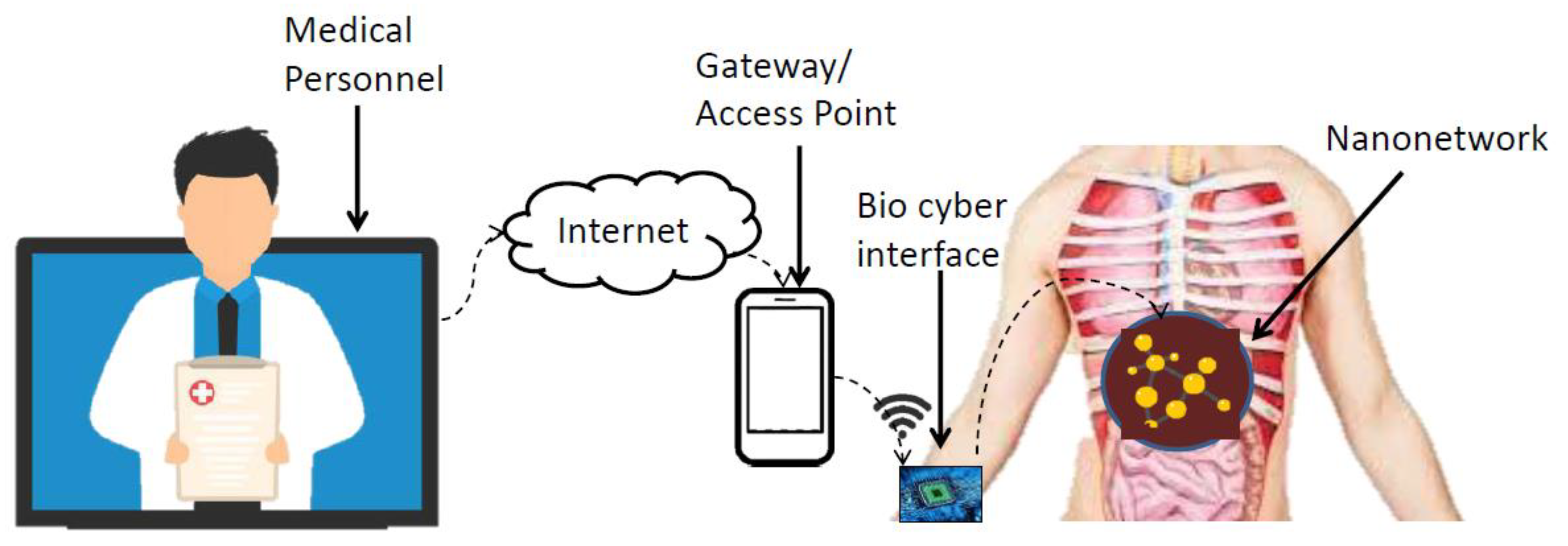
2.1. Internet of Bio Nano Things-Overview
2.2. Related Work
2.3. Deep-Learning Enabled Traffic Analysis
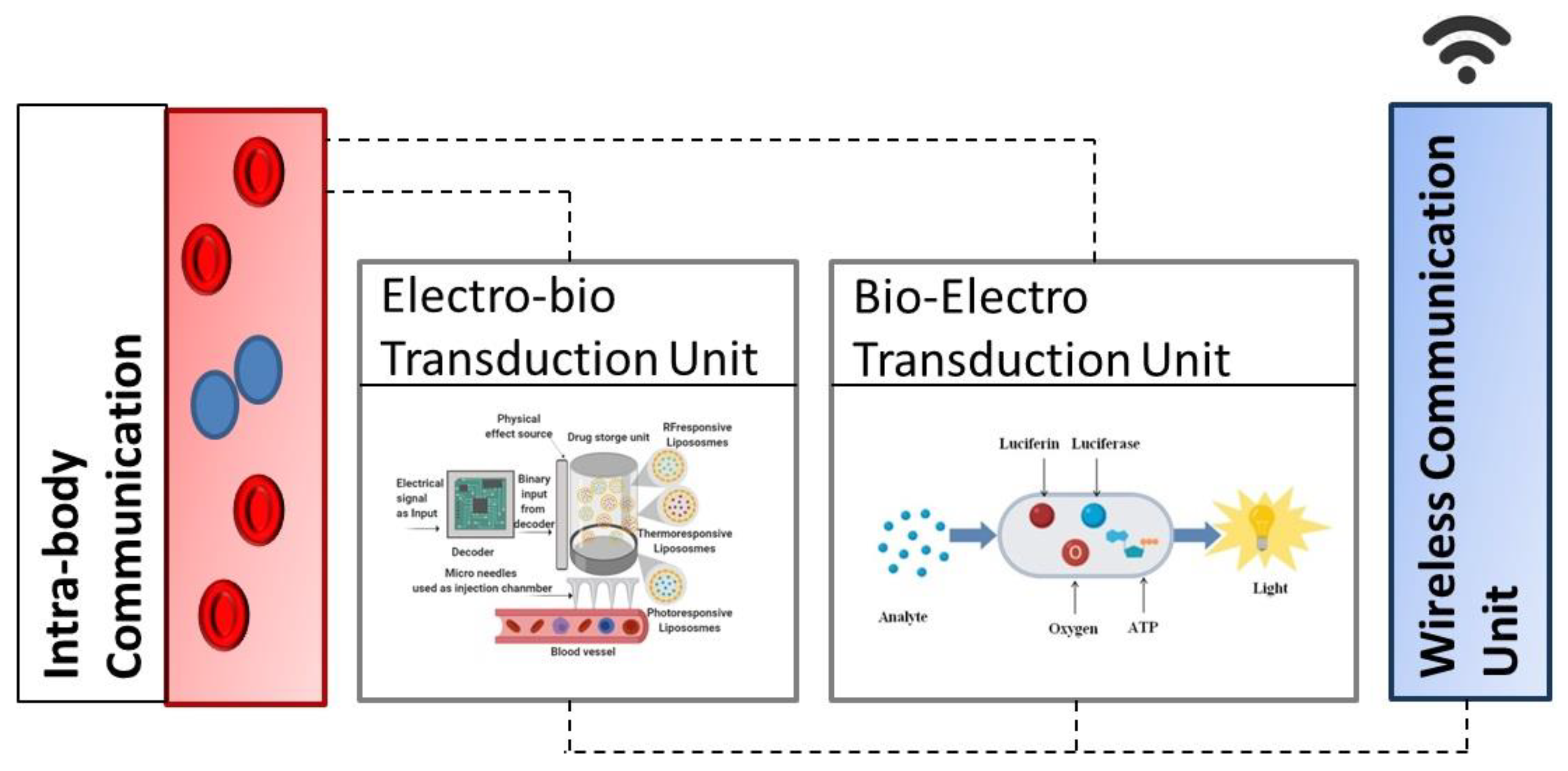
3. Bioluminescence Based Bio–Cyber Interface Architecture
3.1. Electro-Bio Transduction Unit
3.2. Bio-Electro Transduction Unit
4. The Proposed Methodology
4.1. Data Pre-Processor
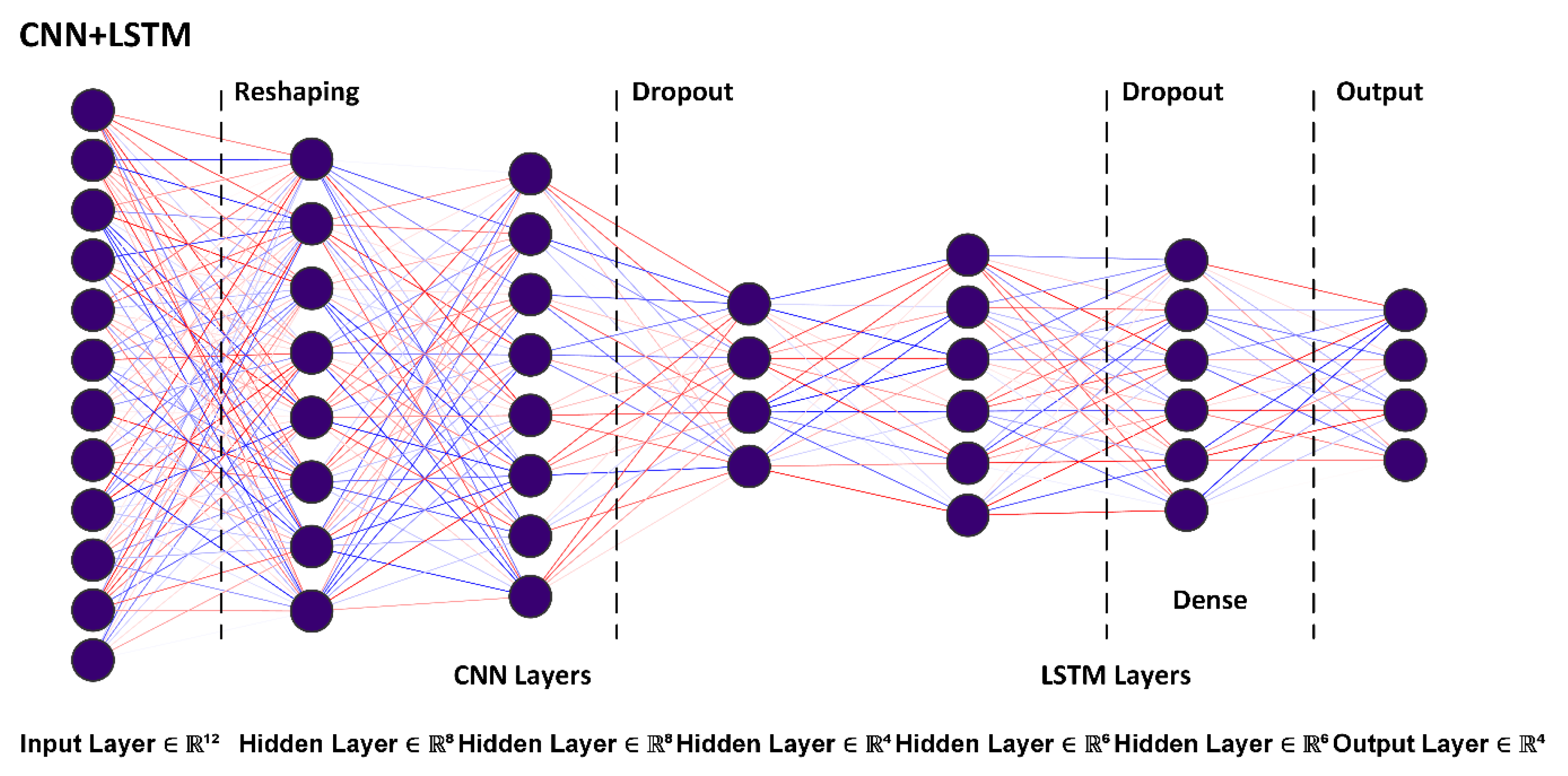
4.2. Neural Network Structures
4.3. Experiment and Measurements
4.3.1. Data Processing
4.3.2. Neural Network Structures and Control Variables
5. Results and Discussion
5.1. Quantitative Results
5.2. Qualitative Observations
5.3. Hybrid Structure: Analysis and Discussion
5.3.1. Performance Comparison
5.3.2. Operational Considerations and Challenges
5.4. System Engineering: Deployment Primitives
6. Conclusions and Future Work
Author Contributions
Funding
Data Availability Statement
Acknowledgments
Conflicts of Interest
References
- Akyildiz, I.F.; Pierobon, M.; Balasubramaniam, S.; Koucheryavy, Y. The internet of Bio-Nano things. IEEE Commun. Mag. 2015, 53, 32–40. [Google Scholar] [CrossRef]
- Nakano, T.; Kobayashi, S.; Suda, T.; Okaie, Y.; Hiraoka, Y.; Haraguchi, T. Externally Controllable Molecular Communication. IEEE J. Sel. Areas Commun. 2014, 32, 2417–2431. [Google Scholar] [CrossRef]
- Akyildiz, I.F.; Brunetti, F.; Blázquez, C. Nanonetworks: A new communication paradigm. Comput. Netw. 2008, 52, 2260–2279. [Google Scholar] [CrossRef]
- Zafar, S.; Nazir, M.; Bakhshi, T.; Khattak, H.A.; Khan, S.; Bilal, M.; Choo, K.-K.R.; Kwak, K.-S.; Sabah, A. A Systematic Review of Bio-Cyber Interface Technologies and Security Issues for Internet of Bio-Nano Things. IEEE Access 2021, 9, 93529–93566. [Google Scholar] [CrossRef]
- Chude-Okonkwo, U.A.K.; Malekian, R.; Maharaj, B.T. Biologically Inspired Bio-Cyber Interface Architecture and Model for Internet of Bio-NanoThings Applications. IEEE Trans. Commun. 2016, 64, 3444–3455. [Google Scholar] [CrossRef]
- Nakano, T.; Moore, M.J.; Wei, F.; Vasilakos, A.V.; Shuai, J. Molecular Communication and Networking: Opportunities and Challenges. IEEE Trans. NanoBiosci. 2012, 11, 135–148. [Google Scholar] [CrossRef]
- Nakano, T.; Okaie, Y.; Vasilakos, A.V. Transmission Rate Control for Molecular Communication among Biological Nanomachines. IEEE J. Sel. Areas Commun. 2013, 31, 835–846. [Google Scholar] [CrossRef]
- Felicetti, L.; Femminella, M.; Reali, G.; Nakano, T.; Vasilakos, A.V. TCP-Like Molecular Communications. IEEE J. Sel. Areas Commun. 2014, 32, 2354–2367. [Google Scholar] [CrossRef]
- Garralda, N.; Llatser, I.; Cabellos-Aparicio, A.; Alarcón, E.; Pierobon, M. Diffusion-based physical channel identification in molecular nanonetworks. Nano Commun. Netw. 2011, 2, 196–204. [Google Scholar] [CrossRef]
- Kuran, M.; Yilmaz, H.B.; Tugcu, T.; Özerman, B. Energy model for communication via diffusion in nanonetworks. Nano Commun. Netw. 2010, 1, 86–95. [Google Scholar] [CrossRef]
- Gregori, M.; Akyildiz, I.F. A new nanonetwork architecture using flagellated bacteria and catalytic nanomotors. IEEE J. Sel. Areas Commun. 2010, 28, 612–619. [Google Scholar] [CrossRef]
- Deshpande, P.P.; Biswas, S.; Torchilin, V.P. Current trends in the use of liposomes for tumor targeting. Nanomedicine 2013, 8, 1509–1528. [Google Scholar] [CrossRef] [PubMed]
- Torchilin, V.P. Multifunctional, stimuli-sensitive nanoparticulate systems for drug delivery. Nat. Rev. Drug Discov. 2014, 13, 813–827. [Google Scholar] [CrossRef] [PubMed]
- Dollard, M.-A.; Billard, P. Whole-cell bacterial sensors for the monitoring of phosphate bioavailability. J. Microbiol. Methods 2003, 55, 221–229. [Google Scholar] [CrossRef] [PubMed]
- Yeo, D.; Wiraja, C.; Chuah, Y.J.; Gao, Y.; Xu, C. A nanoparticle-based sensor platform for cell tracking and status/function assessment. Sci. Rep. 2015, 5, 14768. [Google Scholar] [CrossRef]
- Lee, Y.-E.K.; Smith, R.; Kopelman, R. Nanoparticle PEBBLE sensors in live cells and in vivo. Annu. Rev. Anal. Chem. 2009, 2, 57–76. [Google Scholar] [CrossRef]
- Kuscu, M.; Akan, O.B. Modeling and Analysis of SiNW FET-Based Molecular Communication Receiver. IEEE Trans. Commun. 2016, 64, 3708–3721. [Google Scholar] [CrossRef]
- Liu, Y.; Tsao, C.; Kim, E.; Tschirhart, T.; Terrell, J.L.; Bentley, W.E.; Payne, G.F. Using a Redox Modality to Connect Synthetic Biology to Electronics: Hydrogel-Based Chemo-Electro Signal Transduction for Molecular Communication. Adv. Healthc. Mater. 2017, 6, 1600908. [Google Scholar] [CrossRef]
- Liu, Y.; Li, J.; Tschirhart, T.; Terrell, J.L.; Kim, E.; Tsao, C.; Kelly, D.L.; Bentley, W.E.; Payne, G.F. Connecting Biology to Electronics: Molecular Communication via Redox Modality. Adv. Healthc. Mater. 2017, 6, 1700789. [Google Scholar] [CrossRef]
- Dressler, F.; Kargl, F. Security in nano communication: Challenges and open research issues. In Proceedings of the ICC 2012–2012 IEEE International Conference on Communications, Ottawa, ON, Canada, 10–15 June 2012; pp. 6183–6187. [Google Scholar]
- Loscri, V.; Marchal, C.; Mitton, N.; Fortino, G.; Vasilakos, A.V. Security and Privacy in Molecular Communication and Networking: Opportunities and Challenges. IEEE Trans. NanoBiosci. 2014, 13, 198–207. [Google Scholar] [CrossRef]
- Giaretta, A.; Balasubramaniam, S.; Conti, M. Security Vulnerabilities and Countermeasures for Target Localization in Bio-NanoThings Communication Networks. IEEE Trans. Inf. Forensics Secur. 2016, 11, 665–676. [Google Scholar] [CrossRef]
- Zafar, S.; Aman, W.; Rahman, M.M.U.; Alomainy, A.; Abbasi, Q.H. Channel impulse response-based physical layer authentication in a diffusion-based molecular communication system. In Proceedings of the 2019 UK/China Emerging Technologies (UCET), Glasgow, UK, 21–22 August 2019; pp. 1–2. [Google Scholar]
- El-Fatyany, A.; Wang, H.; El-Atty, S.M.A.; Khan, M. Biocyber Interface-Based Privacy for Internet of Bio-nano Things. Wirel. Pers. Commun. 2020, 114, 1465–1483. [Google Scholar] [CrossRef]
- Bakhshi, T.; Shahid, S. Securing internet of bio-nano things: ML-enabled parameter profiling of bio-cyber interfaces. In Proceedings of the 2019 22nd International Multitopic Conference (INMIC), Islamabad, Pakistan, 29–30 November 2019; pp. 1–8. [Google Scholar]
- Abusitta, A.; de Carvalho, G.H.; Wahab, O.A.; Halabi, T.; Fung, B.C.; Al Mamoori, S. Deep learning-enabled anomaly detection for IoT systems. Internet Things 2023, 21, 100656. [Google Scholar] [CrossRef]
- Rosero-Montalvo, P.D.; István, Z.; Tözün, P.; Hernandez, W. Hybrid Anomaly Detection Model on Trusted IoT Devices. IEEE Internet Things J. 2023, 10, 10959–10969. [Google Scholar] [CrossRef]
- Chander, N.; Kumar, M.U. Metaheuristic feature selection with deep learning enabled cascaded recurrent neural network for anomaly detection in Industrial Internet of Things environment. Clust. Comput. 2023, 26, 1801–1819. [Google Scholar] [CrossRef]
- Hameed, A.; Violos, J.; Leivadeas, A. A Deep Learning Approach for IoT Traffic Multi-Classification in a Smart-City Scenario. IEEE Access 2022, 10, 21193–21210. [Google Scholar] [CrossRef]
- Guan, J.; Cai, J.; Bai, H.; You, I. Deep transfer learning-based network traffic classification for scarce dataset in 5G IoT systems. Int. J. Mach. Learn. Cybern. 2021, 12, 3351–3365. [Google Scholar] [CrossRef]
- Etemadi, A.; Farahnak-Ghazani, M.; Arjmandi, H.; Mirmohseni, M.; Nasiri-Kenari, M. Abnormality Detection and Localization Schemes Using Molecular Communication Systems: A Survey. IEEE Access 2023, 11, 1761–1792. [Google Scholar] [CrossRef]
- Janabi, A.H.; Kanakis, T.; Johnson, M. Convolutional Neural Network Based Algorithm for Early Warning Proactive System Security in Software Defined Networks. IEEE Access 2022, 10, 14301–14310. [Google Scholar] [CrossRef]
- Zafar, S.; Nazir, M.; Sabah, A.; Jurcut, A.D. Securing Bio-Cyber Interface for the Internet of Bio-Nano Things using Particle Swarm Optimization and Artificial Neural Networks based parameter profiling. Comput. Biol. Med. 2021, 136, 104707. [Google Scholar] [CrossRef]
- Lopez-Martin, M.; Carro, B.; Sanchez-Esguevillas, A.; Lloret, J. Network Traffic Classifier With Convolutional and Recurrent Neural Networks for Internet of Things. IEEE Access 2017, 5, 18042–18050. [Google Scholar] [CrossRef]
- Bakhshi, T.; Ghita, B. Anomaly Detection in Encrypted Internet Traffic Using Hybrid Deep Learning. Secur. Commun. Netw. 2021, 2021, 5363750. [Google Scholar] [CrossRef]
- Li, X.; Zhang, D.; Li, M.; Lee, D.-J. Accurate Head Pose Estimation Using Image Rectification and a Lightweight Convolutional Neural Network. IEEE Trans. Multimed. 2022, 25, 2239–2251. [Google Scholar] [CrossRef]
- Goodwin, I.; Bengio, Y.; Courville, A. Deep Learning, 1st ed.; MIT Press: Cambridge, MA, USA, 2016. [Google Scholar]
- Abiodun, O.I.; Jantan, A.; Omolara, A.E.; Dada, K.V.; Mohamed, N.A.; Arshad, H. State-of-the-art in artificial neural network applications: A survey. Heliyon 2018, 4, e00938. [Google Scholar] [CrossRef] [PubMed]
- Tealab, A. Time series forecasting using artificial neural networks methodologies: A systematic review. Future Comput. Inform. J. 2018, 3, 334–340. [Google Scholar] [CrossRef]
- Olvera, D.; Monaghan, M.G. Electroactive material-based biosensors for detection and drug delivery. Adv. Drug Deliv. Rev. 2021, 170, 396–424. [Google Scholar] [CrossRef] [PubMed]
- Nakano, T.; Suda, T.; Okaie, Y.; Moore, M.J.; Vasilakos, A.V. Molecular communication among biological nanomachines: A layered architecture and research issues. IEEE Trans. NanoBiosci. 2014, 13, 169–197. [Google Scholar] [CrossRef] [PubMed]
- Klein, T.; Bradley, G. Cunningham’s Textbook of Veterinary Physiology, 6th ed.; Elsevier Health Sciences: Amsterdam, The Netherlands, 2019; Available online: https://www.uk.elsevierhealth.com/cunninghams-textbook-of-veterinary-physiology-9780323676724.html (accessed on 24 March 2023).
- Marques, S.M.; da Silva, J.C.G.E. Firefly bioluminescence: A mechanistic approach of luciferase catalyzed reactions. IUBMB Life 2009, 61, 6–17. [Google Scholar] [CrossRef]
- Bakhshi, T. Hybrid Deep Learning Techniques for Securing Bioluminescent Interfaces in Internet of Bio Nano Things (1.1) [Data set]. Zenodo 2022. [Google Scholar] [CrossRef]
- Zeng, Y.; Gu, H.; Wei, W.; Guo, Y. $Deep-Full-Range$: A Deep Learning Based Network Encrypted Traffic Classification and Intrusion Detection Framework. IEEE Access 2019, 7, 45182–45190. [Google Scholar] [CrossRef]
- Chollet, F.; Keras. 2015. Available online: https://keras.io (accessed on 24 March 2023).
- Dixit, P.; Silakari, S. Deep Learning Algorithms for Cybersecurity Applications: A Technological and Status Review. Comput. Sci. Rev. 2021, 39, 100317. [Google Scholar] [CrossRef]
- Google. TensorFlow. Available online: https://www.tensorflow.org (accessed on 24 March 2023).
- Springenberg, J.T.; Dosovitskiy, A.; Brox, T.; Riedmiller, M. Striving for Simplicity: The All-Convolutional Net. arXiv 2014, arXiv:1412.6806. [Google Scholar]
- Burr, G.W.; Shelby, R.M.; Sebastian, A.; Kim, S.; Kim, S.; Sidler, S.; Virwani, K.; Ishii, M.; Narayanan, P.; Fumarola, A.; et al. Neuromorphic computing using non-volatile memory. Adv. Physics X 2017, 2, 89–124. [Google Scholar] [CrossRef]
- Intel. Loihi 2: A New Generation of Neuromorphic Computing. Available online: https://www.intel.com/content/www/us/en/research/neuromorphic-computing.html (accessed on 24 March 2023).
- Esser, S.K.; Merolla, P.A.; Arthur, J.V.; Cassidy, A.S.; Appuswamy, R.; Andreopoulos, A.; Berg, D.J.; McKinstry, J.L.; Melano, T.; Barch, D.R.; et al. Convolutional networks for fast, energy-efficient neuromorphic computing. Proc. Natl. Acad. Sci. USA 2016, 113, 11441–11446. [Google Scholar] [CrossRef]
- Boybat, I.; Le Gallo, M.; Nandakumar, S.R.; Moraitis, T.; Parnell, T.; Tuma, T.; Rajendran, B.; Leblebici, Y.; Sebastian, A.; Eleftheriou, E. Neuromorphic computing with multi-memristive synapses. Nat. Commun. 2018, 9, 2514. [Google Scholar] [CrossRef] [PubMed]
- Davison, A.P.; Brüderle, D.; Eppler, J.; Kremkow, J.; Muller, E.; Pecevski, D.; Perrinet, L.; Yger, P. PyNN: A common interface for neuronal network simulators. Front. Neurosci. 2009, 2, 11. [Google Scholar] [CrossRef] [PubMed]
- Wunderlich, T.; Kungl, A.F.; Müller, E.; Hartel, A.; Stradmann, Y.; Aamir, S.A.; Grübl, A.; Heimbrecht, A.; Schreiber, K.; Stöckel, D.; et al. Demonstrating Advantages of Neuromorphic Computation: A Pilot Study. Front. Neurosci. 2019, 13, 260. [Google Scholar] [CrossRef]
- Li, Y.; Ang, K.-W. Hardware Implementation of Neuromorphic Computing Using Large-Scale Memristor Crossbar Arrays. Adv. Intell. Syst. 2021, 3, 2000137. [Google Scholar] [CrossRef]
- Wang, G.; Ma, S.; Wu, Y.; Pei, J.; Zhao, R.; Shi, L. End-to-End Implementation of Various Hybrid Neural Networks on a Cross-Paradigm Neuromorphic Chip. Front. Neurosci. 2021, 15, 615279. [Google Scholar] [CrossRef]
- Wang, Z.; Zhao, W.; Kang, W.; Zhang, Y.; Klein, J.-O.; Chappert, C. Ferroelectric tunnel memristor-based neuromorphic network with 1T1R crossbar architecture. In Proceedings of the 2014 International Joint Conference on Neural Networks (IJCNN), Beijing, China, 6–11 July 2014; pp. 29–34. [Google Scholar]


| Research Domain | Scope of Work | Cross-Connecting Themes |
|---|---|---|
| IoBNT Systems [1,2,3,4,5,6,31] | Comprehensive survey, technology reviews, and use cases | Threat analytics, IoBNT interface, molecular communication, TDD |
| Attack analysis and mitigation [22,23] | Attack taxonomy (black-hole, sentry), countermeasures, authentication schemes | Threat analytics, IoBNT interface, OS fingerprinting, access control |
| BBI Security [24,25] | BBI authentication, design, decision tree-based IDS | ML, traffic classification, logistic mapping, TDD |
| BioFET Security [25,33] | C5.0, ANN, PSO-based IDS for BioFET interfaces | ML, Traffic classification, anomaly detection, deep learning |
| Redox Security [25] | Decision tree and regression-based IDS | ML, traffic classification, feature engineering |
| MC and in-vivo Security [20,21] | Security requirements, deployment | Threat analytics, access control, TDD |
| IoT (IDS, IPS) [26,27,28,29,30,32] | Neural network-based IDS for IoT environments (applications in IIoT, SmartCity, 5G networks) | ML, traffic classification, feature engineering, anomaly detection, deep learning, performance comparison, de-noising (data) |
| Parameter | Description | Value |
|---|---|---|
| Ψ0 | Cumulative concentration of released molecules | 0.62–1.50 mL |
| k10 | Elimination rate | 0.172–0.472 min−1 |
| aM | Michaelis-Menten constant | 10–17 µM |
| k12 | Kinetic constant | 0.073–0.373 min−1 |
| k21 | Forward rate constant | 0.00053–0.00103 min−1 |
| al | Catalytic reaction constant | 4.1–4.4 × 10⁻² µM |
| kl | Ligand–receptor binding constant | 0.001–0.0015 min−1 |
| Atp | Concentration of ATP | 10–40 µL |
| m0 | Concentration of information molecules | 5–10 µM |
| Λ | Release rate | 0.0104–0.0404 min−1 |
| k12,r | Reverse Kinetic constant | 0.00043–0.00103 min−1 |
| k21,r | Forward rate constant | 0.073–0.373 min−1 |
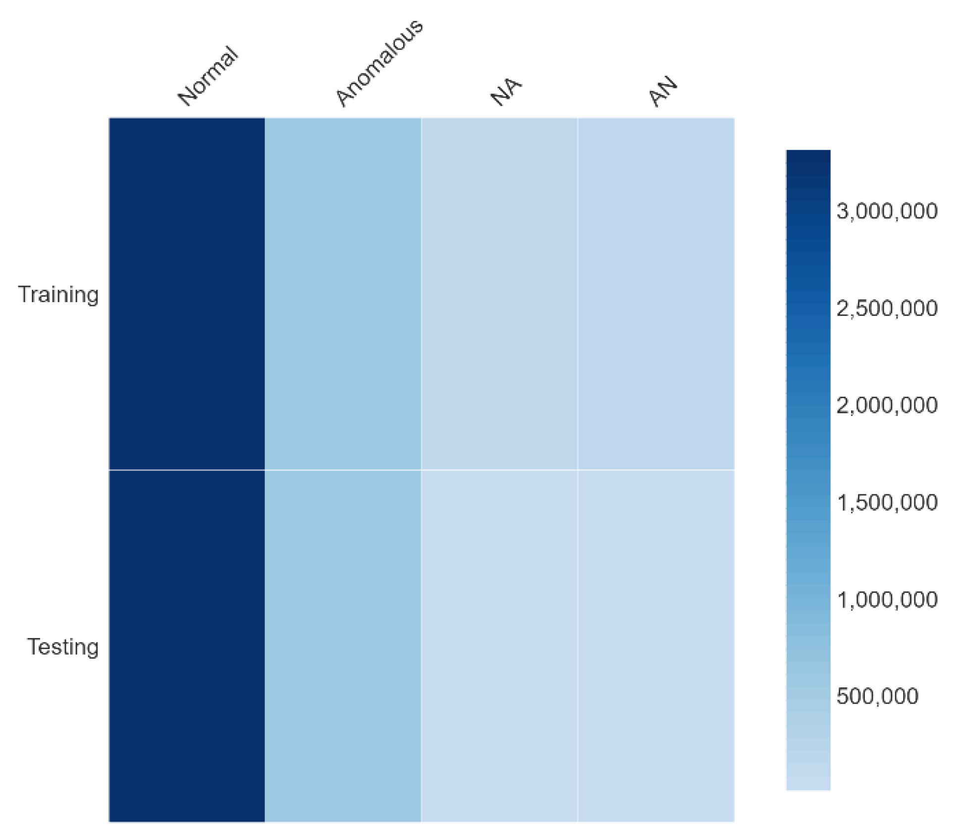
| Distribution | Class Label | Training Data | Test Data |
|---|---|---|---|
| 1 D | Normal + Anomalous | 3,992,268 | 3,992,271 |
| 2 D | Normal | - | 3,433,351 |
| - | Anomalous | 558,917 | |
| 4 D | Normal | - | 3,316,617 |
| Normal {abnormal parameters > 25%} | - | 116,734 | |
| - | Anomalous | 538,796 | |
| - | Anomalous {abnormal parameters < 25%} | 20,121 | |
| Total | - | - | 6,866,701 |
| Property | Parameters | Comments |
|---|---|---|
| System | Core i7-960 16 MB 3.2 GHz 64 GB | Intel architecture DDR3L 1066 |
| Ubuntu 18.04.5 | Kernel 4.15.0-135- 64 | |
| Keras 2.4.0. | DL API (Python) [32] | |
| TensorFlow 2.8.0. | ML Library (Opensource) [33] | |
| Data Processing | Data density distribution | Gaussian PDF |
| RobustScalar (options) | SciPi toolkits using RobustScalar class [37] | |
| with_centering | controls value centering at 0 (median is subtracted) and set to default True. | |
| with_scaling | controls IQR scaling (standard deviation of 1) and set to default True. | |
| quantile_range | Tuple (0–100), default (25, and 75) | |
| Data encoding | Non-intrinsic traffic labeling using the OneHotEncoder class [37] | |
| Neural Network Convolutional/Recurrent | Rectified Linear Unit (ReLU) | Non-linear (piece-wise linear) activation function used in DL classifiers [37] |
| FATE/FederatedAI | The final layer in the DL model to aid logistic regression [45] | |
| Dropout = 0.5 | Regularization method reducing over-fitting by minimizing weight learning per iteration [14,16,37] | |
| Softmax output function | The normalized exponential function used as the last activation in neural networks to normalize output [37] | |
| Optimizer = Nadam | Gradient descent algorithm employed to minimize cost function [37,38]. | |
| Loss function = Categorical cross-entropy | Loss function to benchmark neural network reduction in the training phase [37,39] |
| Metric and Description | Calculation |
|---|---|
| Accuracy: The ratio is correctly identified and divided into total samples. | |
| Precision: Positive predictions (correctly identified). | |
| Recall: Ratio of anomalies correctly classified to total samples. | |
| F1-Score: Metric defining mean value determined for P and R times two. | |
| False Positive Rate (FPR): Ratio of anomalous to normal samples. | |
| Normalization factor: The data set is normalized using the max. and min. of input (column-wise), then to each data value. | |
| Time- Latency: The total time involved in training and testing a neural network | Training duration = TD Testing duration = TD’ |
| Metric | Neural Network Structure | |||||
|---|---|---|---|---|---|---|
| Non-Hybrid | Hybrid | |||||
| 1D CNN | CNN | LSTM | GRU | CNN + LSTM | CNN + GRU | |
| TD (s) | 26.81 | 215.89 | 785.61 | 921.24 | 315.6 | 468.12 |
| TD’(s) | 11.5 | 116.81 | 256.84 | 312.89 | 129.31 | 221.51 |
| A (%) | 73.42 | 91.56 | 82.24 | 81.17 | 93.51 | 87.52 |
| P (%) | 69.14 | 92.21 | 89.31 | 81.62 | 91.81 | 89.61 |
| R (%) | 76.15 | 88.15 | 89.62 | 88.11 | 90.11 | 82.61 |
| FPR (%) | 1.21 | 1.45 | 14.12 | 6.89 | 1.10 | 2.81 |
| F1- (%) | 81.98 | 92.21 | 90.51 | 87.58 | 92.01 | 89.51 |
| Contribution | Domain | Classifier | Constraint(s) | Features |
|---|---|---|---|---|
| Zafar et al. [23] | IoBNT | Impulse response fingerprinting | Significant probability of incorrect detection in noisy data | CIR fingerprinting for anomalous control signal discrimination |
| El-Fatyany et al. [24] | IoBNT | Logistic mapping and BPSK modulation | Multi-stage encryption, in-vivo TDD disruption, compute overhead | BPSK session key encryption for IoBNT interface signaling |
| Bakhshi et al. [25] | IoBNT | ML (supervised learning—C5.0) | Manually crafted features, limited dataset, satisfactory efficiency | Security profiling BBI, BioFET, and Redox IoBNT interfaces |
| Abusitta et al. [26] | IoT | Semi-Hybrid: ML (un-supervised) + DNN | Unsupervised ML-based feature engg., 2D classification | De-noising traffic parameters followed by the NN application |
| Rosero et al. [27] | IoT | Semi-Hybrid: ML (unsupervised) + DNN | Multi-stage feature processing, computation overhead | kNN, NB, SVM, heuristics-based outlier detection, followed by RNN |
| Chander et al. [28] | IIoT | RNN (GRU) | Multi-stage metaheuristic feature optimization challenges | Use of deer hunting (feature) optimization followed by GRU RNN |
| Hameed et al. [29] | IoT | Logistic regression + MLP ANN | Supervised learning for feature selection, frequent re-training | Scheme outperforms ML methods in smart city IoT deployments |
| Guan et al. [30] | IoT | CNN, LSTM | Reliance on determining appropriate data transfer models from other domain(s) | High classification accuracy using transfer learning approaches from existing classifiers |
| Zafar et al. [33] | IoBNT | PSO, ANN | Limited data, and feature diversity | NN-based profiling of BioFET interfacing for anomaly detection |
| Proposed Hybrid Classifier | IoBNT | CNN, LSTM | Latency-efficiency trade-off compared to 1D CNN | High-accuracy single-stage hybrid structure, eliminating manual feature engineering |
Disclaimer/Publisher’s Note: The statements, opinions and data contained in all publications are solely those of the individual author(s) and contributor(s) and not of MDPI and/or the editor(s). MDPI and/or the editor(s) disclaim responsibility for any injury to people or property resulting from any ideas, methods, instructions or products referred to in the content. |
© 2023 by the authors. Licensee MDPI, Basel, Switzerland. This article is an open access article distributed under the terms and conditions of the Creative Commons Attribution (CC BY) license (https://creativecommons.org/licenses/by/4.0/).
Share and Cite
Bakhshi, T.; Zafar, S. Hybrid Deep Learning Techniques for Securing Bioluminescent Interfaces in Internet of Bio Nano Things. Sensors 2023, 23, 8972. https://doi.org/10.3390/s23218972
Bakhshi T, Zafar S. Hybrid Deep Learning Techniques for Securing Bioluminescent Interfaces in Internet of Bio Nano Things. Sensors. 2023; 23(21):8972. https://doi.org/10.3390/s23218972
Chicago/Turabian StyleBakhshi, Taimur, and Sidra Zafar. 2023. "Hybrid Deep Learning Techniques for Securing Bioluminescent Interfaces in Internet of Bio Nano Things" Sensors 23, no. 21: 8972. https://doi.org/10.3390/s23218972
APA StyleBakhshi, T., & Zafar, S. (2023). Hybrid Deep Learning Techniques for Securing Bioluminescent Interfaces in Internet of Bio Nano Things. Sensors, 23(21), 8972. https://doi.org/10.3390/s23218972