
Enhancing Wearable Gait Monitoring Systems: Identifying Optimal Kinematic Inputs in Typical Adolescents


 , and
, and 
Abstract
:1. Introduction
2. Materials and Methods
2.1. Participants
2.2. Instrumentation
2.3. Data Collection
2.4. Data Processing
2.4.1. Signal Conditioning
2.4.2. Similarity Analysis
Distance Similarity
Poincare Similarity
2.4.3. Spatiotemporal Parameters
2.5. Statistical Analysis
3. Results
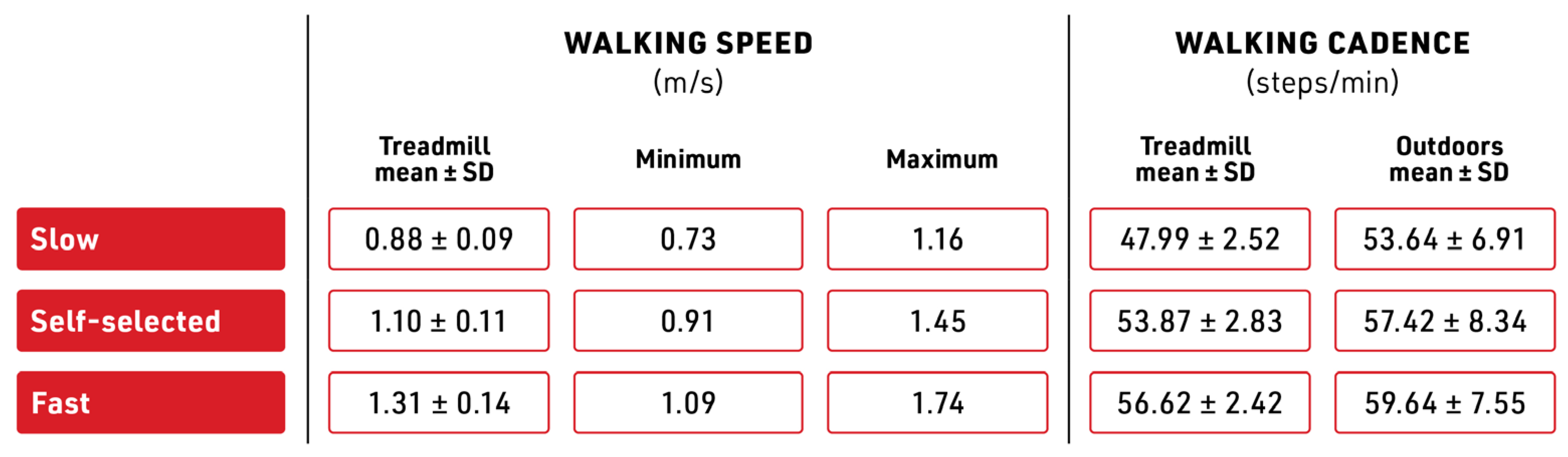
3.1. Walking Speed
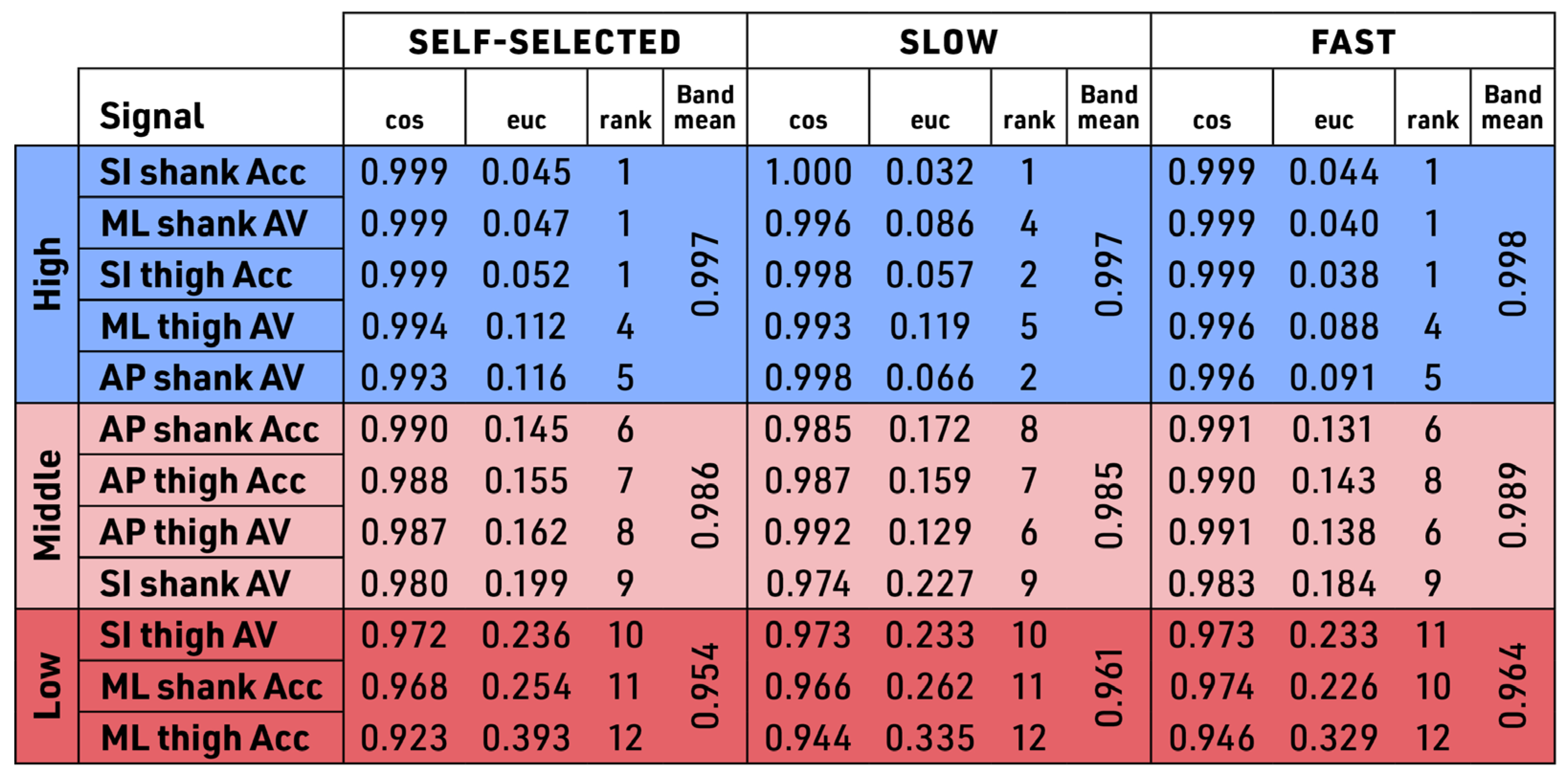
3.2. Signal Similarity Measures
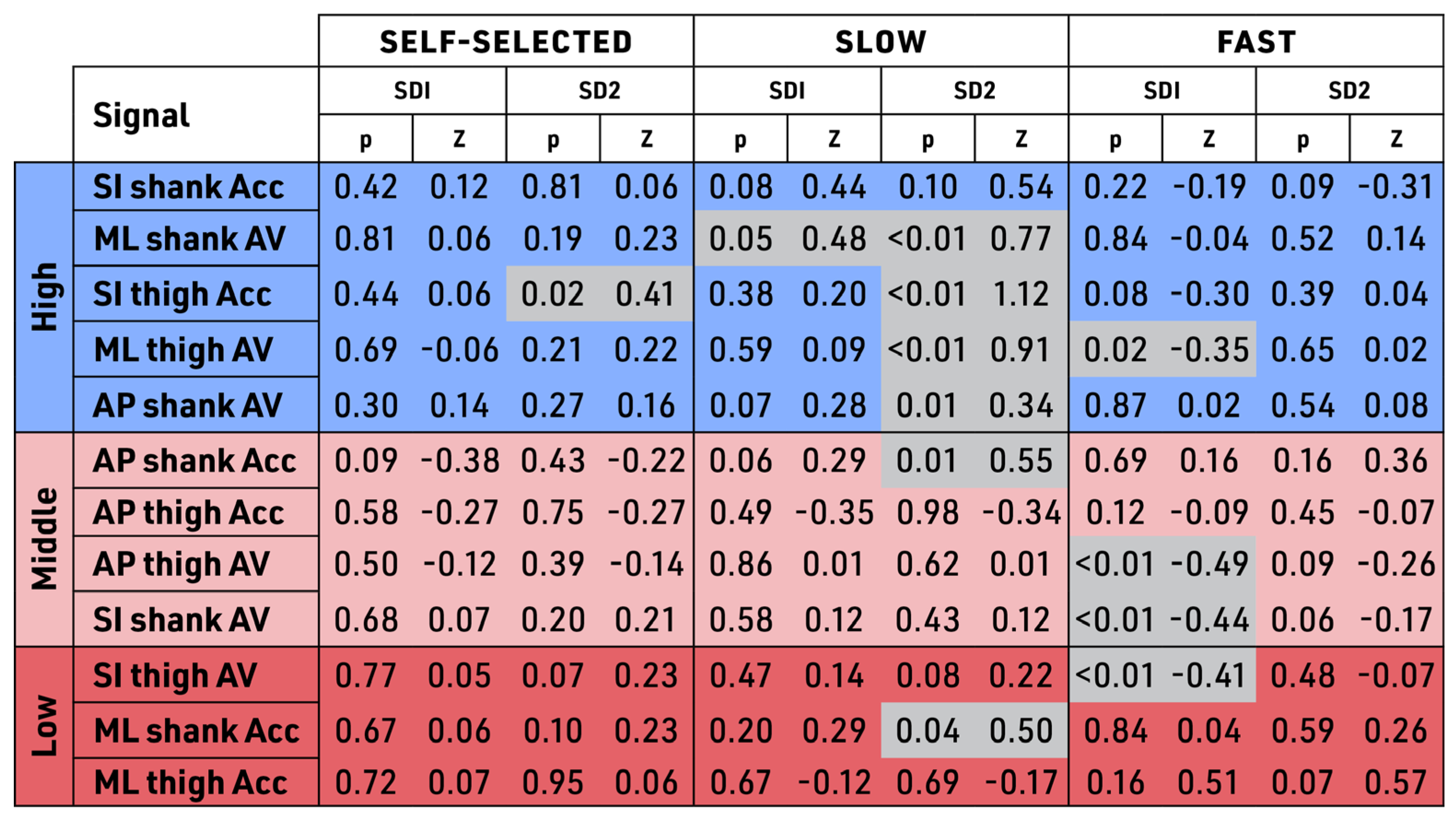
3.3. Poincare Analysis
3.4. Spatiotemporal Parameters
4. Discussion
4.1. Identifying the Optimal Kinematic Signals for IMU-Based Gait Monitoring Models
4.2. ML Shank AV and SI Shank Acc
4.3. Similarity Measures
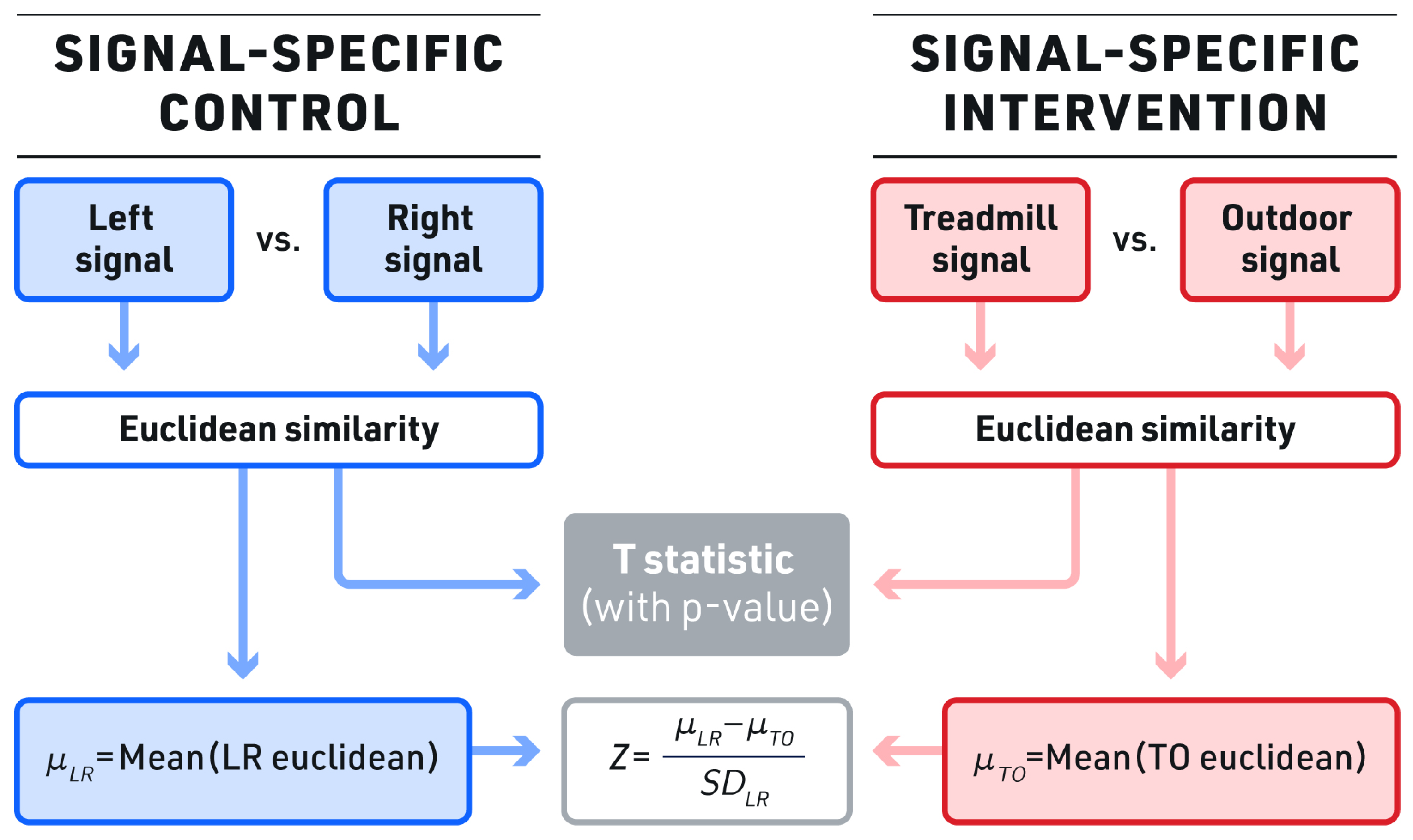
4.4. Bilateral Symmetry Dissimilarity Testing (BSDT)
4.5. Signals: ML Shank AV and SI Shank Acc
4.6. Spatiotemporal Differences in Gait
4.7. Limitations
4.7.1. Sample Size Limitations
4.7.2. Subjectivity of IMU Studies as a Limitation
4.7.3. BSDT Limitation
4.8. Future Work
5. Conclusions
Author Contributions
Funding
Institutional Review Board Statement
Informed Consent Statement
Data Availability Statement
Acknowledgments
Conflicts of Interest
References
- Buongiorno, D.; Bortone, I.; Cascarano, G.D.; Trotta, G.F.; Brunetti, A.; Bevilacqua, V. A Low-Cost Vision System Based on the Analysis of Motor Features for Recognition and Severity Rating of Parkinson’s Disease. BMC Med. Inform. Decis. Mak. 2019, 19, 243. [Google Scholar] [CrossRef]
- Dobkin, B.H.; Martinez, C. Wearable Sensors to Monitor, Enable Feedback, and Measure Outcomes of Activity and Practice. Curr. Neurol. Neurosci. Rep. 2018, 18, 87. [Google Scholar] [CrossRef] [PubMed]
- Juen, J.; Cheng, Q.; Prieto-Centurion, V.; Krishnan, J.A.; Schatz, B. Health Monitors for Chronic Disease by Gait Analysis with Mobile Phones. Telemed. E-Health 2014, 20, 1035–1041. [Google Scholar] [CrossRef]
- Kumari, P.; Cooney, N.J.; Kim, T.; Minhas, A.S. Gait Analysis in Spastic Hemiplegia and Diplegia Cerebral Palsy Using a Wearable Activity Tracking Device—A Data Quality Analysis for Deep Convolutional Neural Networks. In Proceedings of the 2018 5th Asia-Pacific World Congress on Computer Science and Engineering (APWC on CSE), Nadi, Fiji, 10–12 December 2018; pp. 1–4. [Google Scholar] [CrossRef]
- Zhen, T.; Yan, L.; Yuan, P. Walking Gait Phase Detection Based on Acceleration Signals Using LSTM-DNN Algorithm. Algorithms 2019, 12, 253. [Google Scholar] [CrossRef]
- BenAbdelkader, C.; Cutler, R.G.; Davis, L.S. Gait Recognition Using Image Self-Similarity. EURASIP J. Adv. Signal Process. 2004, 2004, 721765. [Google Scholar] [CrossRef]
- Mufandaidza, M.P.; Ramotsoela, T.D.; Hancke, G.P. Continuous User Authentication in Smartphones Using Gait Analysis. In Proceedings of the IECON 2018—44th Annual Conference of the IEEE Industrial Electronics Society, Washington, DC, USA, 21–23 October 2018; pp. 4656–4661. [Google Scholar] [CrossRef]
- Mason, R.; Pearson, L.T.; Barry, G.; Young, F.; Lennon, O.; Godfrey, A.; Stuart, S. Wearables for Running Gait Analysis: A Systematic Review. Sports Med. 2023, 53, 241–268. [Google Scholar] [CrossRef]
- Behboodi, A.; Zahradka, N.; Wright, H.; Alesi, J.; Lee, S.C.K. Real-Time Detection of Seven Phases of Gait in Children with Cerebral Palsy Using Two Gyroscopes. Sensors 2019, 19, 2517. [Google Scholar] [CrossRef]
- Kahlon, A.; Sansare, A.; Behboodi, A. Remote Gait Analysis as a Proxy for Traditional Gait Laboratories: Utilizing Smartphones for Subject-Driven Gait Assessment across Differing Terrains. Biomechanics 2022, 2, 235–254. [Google Scholar] [CrossRef]
- Behboodi, A.; Zahradka, N.; Alesi, J.; Wright, H.; Lee, S.C.K. Use of a Novel Functional Electrical Stimulation Gait Training System in 2 Adolescents with Cerebral Palsy: A Case Series Exploring Neurotherapeutic Changes. Phys. Ther. 2019, 99, 739–747. [Google Scholar] [CrossRef]
- Holmes, H.H.; Fawcett, R.T.; Roper, J.A. Changes in Spatiotemporal Measures and Variability During User-Driven Treadmill, Fixed-Speed Treadmill, and Overground Walking in Young Adults: A Pilot Study. J. Appl. Biomech. 2021, 37, 277–281. [Google Scholar] [CrossRef]
- Bovi, G.; Rabuffetti, M.; Mazzoleni, P.; Ferrarin, M. A Multiple-Task Gait Analysis Approach: Kinematic, Kinetic and EMG Reference Data for Healthy Young and Adult Subjects. Gait Posture 2011, 33, 6–13. [Google Scholar] [CrossRef]
- Hu, H.; Zheng, J.; Zhan, E.; Yu, L. Curve Similarity Model for Real-Time Gait Phase Detection Based on Ground Contact Forces. Sensors 2019, 19, 3235. [Google Scholar] [CrossRef]
- Saboor, A.; Kask, T.; Kuusik, A.; Alam, M.M.; Le Moullec, Y.; Niazi, I.K.; Zoha, A.; Ahmad, R. Latest Research Trends in Gait Analysis Using Wearable Sensors and Machine Learning: A Systematic Review. IEEE Access 2020, 8, 167830–167864. [Google Scholar] [CrossRef]
- Voss, S.; Joyce, J.; Biskis, A.; Parulekar, M.; Armijo, N.; Zampieri, C.; Tracy, R.; Palmer, A.S.; Fefferman, M.; Ouyang, B.; et al. Normative Database of Spatiotemporal Gait Parameters Using Inertial Sensors in Typically Developing Children and Young Adults. Gait Posture 2020, 80, 206–213. [Google Scholar] [CrossRef] [PubMed]
- Peraza, L.R.; Kinnunen, K.M.; McNaney, R.; Craddock, I.J.; Whone, A.L.; Morgan, C.; Joules, R.; Wolz, R. An Automatic Gait Analysis Pipeline for Wearable Sensors: A Pilot Study in Parkinson’s Disease. Sensors 2021, 21, 8286. [Google Scholar] [CrossRef]
- Vu, H.; Gomez, F.; Cherelle, P.; Lefeber, D.; Nowé, A.; Vanderborght, B. ED-FNN: A New Deep Learning Algorithm to Detect Percentage of the Gait Cycle for Powered Prostheses. Sensors 2018, 18, 2389. [Google Scholar] [CrossRef]
- Carcreff, L.; Gerber, C.; Paraschiv-Ionescu, A.; De Coulon, G.; Newman, C.; Armand, S.; Aminian, K. What Is the Best Configuration of Wearable Sensors to Measure Spatiotemporal Gait Parameters in Children with Cerebral Palsy? Sensors 2018, 18, 394. [Google Scholar] [CrossRef] [PubMed]
- Junior, P.R.F.; de Moura, R.C.F.; Oliveira, C.S.; Politti, F. Use of Wearable Inertial Sensors for the Assessment of Spatiotemporal Gait Variables in Children: A Systematic Review. Mot. Rev. Educ. Física 2020, 26, e10200139. [Google Scholar] [CrossRef]
- Semaan, M.B.; Wallard, L.; Ruiz, V.; Gillet, C.; Leteneur, S.; Simoneau-Buessinger, E. Is Treadmill Walking Biomechanically Comparable to Overground Walking? A Systematic Review. Gait Posture 2022, 92, 249–257. [Google Scholar] [CrossRef] [PubMed]
- Benson, L.C.; Clermont, C.A.; Bošnjak, E.; Ferber, R. The Use of Wearable Devices for Walking and Running Gait Analysis Outside of the Lab: A Systematic Review. Gait Posture 2018, 63, 124–138. [Google Scholar] [CrossRef]
- Del Din, S.; Hickey, A.; Ladha, C.; Stuart, S.; Bourke, A.K.; Esser, P.; Rochester, L.; Godfrey, A. Instrumented Gait Assessment with a Single Wearable: An Introductory Tutorial. F1000Research 2016, 5, 2323. [Google Scholar] [CrossRef]
- Chen, S.; Lach, J.; Lo, B.; Yang, G.-Z. Toward Pervasive Gait Analysis with Wearable Sensors: A Systematic Review. IEEE J. Biomed. Health Inform. 2016, 20, 1521–1537. [Google Scholar] [CrossRef]
- Hegde, N.; Zhang, T.; Uswatte, G.; Taub, E.; Barman, J.; McKay, S.; Taylor, A.; Morris, D.M.; Griffin, A.; Sazonov, E.S. The Pediatric SmartShoe: Wearable Sensor System for Ambulatory Monitoring of Physical Activity and Gait. IEEE Trans. Neural Syst. Rehabil. Eng. 2018, 26, 477–486. [Google Scholar] [CrossRef]
- Matsushita, Y.; Tran, D.T.; Yamazoe, H.; Lee, J.-H. Recent Use of Deep Learning Techniques in Clinical Applications Based on Gait: A Survey. J. Comput. Des. Eng. 2021, 8, 1499–1532. [Google Scholar] [CrossRef]
- Aminian, K.; Najafi, B.; Büla, C.; Leyvraz, P.-F.; Robert, P. Spatio-Temporal Parameters of Gait Measured by an Ambulatory System Using Miniature Gyroscopes. J. Biomech. 2002, 35, 689–699. [Google Scholar] [CrossRef]
- Rastegari, E.; Azizian, S.; Ali, H. Machine Learning and Similarity Network Approaches to Support Automatic Classification of Parkinson’s Diseases Using Accelerometer-Based Gait Analysis. In Proceedings of the 52nd Hawaii International Conference on System Sciences, Maui, HI, USA, 8–11 January 2019. [Google Scholar]
- Zhao, Y.; Zhou, S. Wearable Device-Based Gait Recognition Using Angle Embedded Gait Dynamic Images and a Convolutional Neural Network. Sensors 2017, 17, 478. [Google Scholar] [CrossRef]
- Dehzangi, O.; Taherisadr, M.; ChangalVala, R. IMU-Based Gait Recognition Using Convolutional Neural Networks and Multi-Sensor Fusion. Sensors 2017, 17, 2735. [Google Scholar] [CrossRef]
- Adhikary, S.; Ghosh, R.; Ghosh, A. Gait Abnormality Detection without Clinical Intervention Using Wearable Sensors and Machine Learning. In Innovations in Sustainable Energy and Technology; Muthukumar, P., Sarkar, D.K., De, D., De, C.K., Eds.; Advances in Sustainability Science and Technology; Springer: Singapore, 2021; pp. 359–368. [Google Scholar] [CrossRef]
- Yang, S.; Li, Q. Inertial Sensor-Based Methods in Walking Speed Estimation: A Systematic Review. Sensors 2012, 12, 6102–6116. [Google Scholar] [CrossRef]
- Schmitt, A.C.; Baudendistel, S.T.; Lipat, A.L.; White, T.A.; Raffegeau, T.E.; Hass, C.J. Walking Indoors, Outdoors, and on a Treadmill: Gait Differences in Healthy Young and Older Adults. Gait Posture 2021, 90, 468–474. [Google Scholar] [CrossRef] [PubMed]
- Fukuchi, C.A.; Fukuchi, R.K.; Duarte, M. Effects of Walking Speed on Gait Biomechanics in Healthy Participants: A Systematic Review and Meta-Analysis. Syst. Rev. 2019, 8, 153. [Google Scholar] [CrossRef] [PubMed]
- Stansfield, B.W.; Hillman, S.J.; Hazlewood, M.E.; Lawson, A.A.; Mann, A.M.; Loudon, I.R.; Robb, J.E. Normalized Speed, Not Age, Characterizes Ground Reaction Force Patterns in 5-to 12-Year-Old Children Walking at Self-Selected Speeds. J. Pediatr. Orthop. 2001, 21, 395–402. [Google Scholar] [CrossRef]
- van der Linden, M.L.; Kerr, A.M.; Hazlewood, M.E.; Hillman, S.J.; Robb, J.E. Kinematic and Kinetic Gait Characteristics of Normal Children Walking at a Range of Clinically Relevant Speeds. J. Pediatr. Orthop. 2002, 22, 800–806. [Google Scholar] [CrossRef] [PubMed]
- Hollman, J.H.; Watkins, M.K.; Imhoff, A.C.; Braun, C.E.; Akervik, K.A.; Ness, D.K. A Comparison of Variability in Spatiotemporal Gait Parameters between Treadmill and Overground Walking Conditions. Gait Posture 2016, 43, 204–209. [Google Scholar] [CrossRef] [PubMed]
- Schwartz, M.H.; Rozumalski, A. The Gait Deviation Index: A New Comprehensive Index of Gait Pathology. Gait Posture 2008, 28, 351–357. [Google Scholar] [CrossRef] [PubMed]
- Baker, R.; McGinley, J.L.; Schwartz, M.H.; Beynon, S.; Rozumalski, A.; Graham, H.K.; Tirosh, O. The Gait Profile Score and Movement Analysis Profile. Gait Posture 2009, 30, 265–269. [Google Scholar] [CrossRef]
- Barton, G.J.; Hawken, M.B.; Scott, M.A.; Schwartz, M.H. Movement Deviation Profile: A Measure of Distance from Normality Using a Self-Organizing Neural Network. Hum. Mov. Sci. 2012, 31, 284–294. [Google Scholar] [CrossRef]
- Singh, M.K.; Singh, N.; Singh, A.K. Speaker’s Voice Characteristics and Similarity Measurement Using Euclidean Distances. In Proceedings of the 2019 International Conference on Signal Processing and Communication (ICSC), Noida, India, 7–9 March 2019; pp. 317–322. [Google Scholar] [CrossRef]
- Di Marco, R.; Scalona, E.; Pacilli, A.; Cappa, P.; Mazzà, C.; Rossi, S. How to Choose and Interpret Similarity Indices to Quantify the Variability in Gait Joint Kinematics. Int. Biomech. 2018, 5, 1–8. [Google Scholar] [CrossRef]
- Bächlin, M.; Schumm, J.; Roggen, D.; Töster, G. Quantifying Gait Similarity: User Authentication and Real-World Challenge. In Advances in Biometrics; Tistarelli, M., Nixon, M.S., Eds.; Lecture Notes in Computer Science; Springer: Berlin/Heidelberg, Germany, 2009; Volume 5558, pp. 1040–1049. [Google Scholar] [CrossRef]
- Lee, S.; Shin, S. Gait Signal Analysis with Similarity Measure. Sci. World J. 2014, 2014, 136018. [Google Scholar] [CrossRef]
- Riley, P.O.; Paolini, G.; Della Croce, U.; Paylo, K.W.; Kerrigan, D.C. A Kinematic and Kinetic Comparison of Overground and Treadmill Walking in Healthy Subjects. Gait Posture 2007, 26, 17–24. [Google Scholar] [CrossRef]
- Cabral, S. Gait Symmetry Measures and Their Relevance to Gait Retraining. In Handbook of Human Motion; Springer International Publishing: Cham, Switzerland, 2018; pp. 429–447. [Google Scholar] [CrossRef]
- Zahradka, N.; Verma, K.; Behboodi, A.; Bodt, B.; Wright, H.; Lee, S.C.K. An Evaluation of Three Kinematic Methods for Gait Event Detection Compared to the Kinetic-Based ‘Gold Standard’. Sensors 2020, 20, 5272. [Google Scholar] [CrossRef]
- Rueterbories, J.; Spaich, E.G.; Larsen, B.; Andersen, O.K. Methods for Gait Event Detection and Analysis in Ambulatory Systems. Med. Eng. Phys. 2010, 32, 545–552. [Google Scholar] [CrossRef] [PubMed]
- Grimmer, M.; Schmidt, K.; Duarte, J.E.; Neuner, L.; Koginov, G.; Riener, R. Stance and Swing Detection Based on the Angular Velocity of Lower Limb Segments During Walking. Front. Neurorobot. 2019, 13, 57. [Google Scholar] [CrossRef]
- Johnson, C.D.; Outerleys, J.; Davis, I.S. Relationships between Tibial Acceleration and Ground Reaction Force Measures in the Medial-Lateral and Anterior-Posterior Planes. J. Biomech. 2021, 117, 110250. [Google Scholar] [CrossRef] [PubMed]
- Gurchiek, R.D.; Choquette, R.H.; Beynnon, B.D.; Slauterbeck, J.R.; Tourville, T.W.; Toth, M.J.; McGinnis, R.S. Open-Source Remote Gait Analysis: A Post-Surgery Patient Monitoring Application. Sci. Rep. 2019, 9, 17966. [Google Scholar] [CrossRef]
- Sharifi Renani, M.; Myers, C.A.; Zandie, R.; Mahoor, M.H.; Davidson, B.S.; Clary, C.W. Deep Learning in Gait Parameter Prediction for OA and TKA Patients Wearing IMU Sensors. Sensors 2020, 20, 5553. [Google Scholar] [CrossRef] [PubMed]
- Wang, C.; Chan, P.P.K.; Lam, B.M.F.; Wang, S.; Zhang, J.H.; Chan, Z.Y.S.; Chan, R.H.M.; Ho, K.K.W.; Cheung, R.T.H. Real-Time Estimation of Knee Adduction Moment for Gait Retraining in Patients with Knee Osteoarthritis. IEEE Trans. Neural Syst. Rehabil. Eng. 2020, 28, 888–894. [Google Scholar] [CrossRef] [PubMed]
- Asuncion, L.V.R.; Mesa, J.X.P.D.; Juan, P.K.H.; Sayson, N.T.; Cruz, A.R.D. Thigh Motion-Based Gait Analysis for Human Identification Using Inertial Measurement Units (IMUs). In Proceedings of the 2018 IEEE 10th International Conference on Humanoid, Nanotechnology, Information Technology, Communication and Control, Environment and Management (HNICEM), Baguio City, Philippines, 29 November–2 December 2018; pp. 1–6. [Google Scholar] [CrossRef]
- Borzì, L.; Mazzetta, I.; Zampogna, A.; Suppa, A.; Olmo, G.; Irrera, F. Prediction of Freezing of Gait in Parkinson’s Disease Using Wearables and Machine Learning. Sensors 2021, 21, 614. [Google Scholar] [CrossRef] [PubMed]
- Uchitomi, H.; Hirobe, Y.; Miyake, Y. Three-Dimensional Continuous Gait Trajectory Estimation Using Single Shank-Worn Inertial Measurement Units and Clinical Walk Test Application. Sci. Rep. 2022, 12, 5368. [Google Scholar] [CrossRef]
- Wang, L.; Sun, Y.; Li, Q.; Liu, T.; Yi, J. IMU-Based Gait Normalcy Index Calculation for Clinical Evaluation of Impaired Gait. IEEE J. Biomed. Health Inform. 2021, 25, 3–12. [Google Scholar] [CrossRef]
- Allseits, E.; Agrawal, V.; Lučarević, J.; Gailey, R.; Gaunaurd, I.; Bennett, C. A Practical Step Length Algorithm Using Lower Limb Angular Velocities. J. Biomech. 2018, 66, 137–144. [Google Scholar] [CrossRef]
- Jasiewicz, J.M.; Allum, J.H.J.; Middleton, J.W.; Barriskill, A.; Condie, P.; Purcell, B.; Li, R.C.T. Gait Event Detection Using Linear Accelerometers or Angular Velocity Transducers in Able-Bodied and Spinal-Cord Injured Individuals. Gait Posture 2006, 24, 502–509. [Google Scholar] [CrossRef]
- Lee, J.K.; Park, E.J. Quasi Real-Time Gait Event Detection Using Shank-Attached Gyroscopes. Med. Biol. Eng. Comput. 2011, 49, 707–712. [Google Scholar] [CrossRef]
- Han, Y.C.; Wong, K.I.; Murray, I. Gait Phase Detection for Normal and Abnormal Gaits Using IMU. IEEE Sens. J. 2019, 19, 3439–3448. [Google Scholar] [CrossRef]
- Iosa, M.; Cereatti, A.; Merlo, A.; Campanini, I.; Paolucci, S.; Cappozzo, A. Assessment of Waveform Similarity in Clinical Gait Data: The Linear Fit Method. BioMed Res. Int. 2014, 2014, 214156. [Google Scholar] [CrossRef]
- Hill, C.N.; Ross, S.; Peebles, A.; Queen, R.M. Continuous Similarity Analysis in Patient Populations. J. Biomech. 2022, 131, 110916. [Google Scholar] [CrossRef] [PubMed]
- Yu, L.; Zheng, J.; Wang, Y.; Song, Z.; Zhan, E. Adaptive Method for Real-Time Gait Phase Detection Based on Ground Contact Forces. Gait Posture 2015, 41, 269–275. [Google Scholar] [CrossRef] [PubMed]
- Donisi, L.; Pagano, G.; Cesarelli, G.; Coccia, A.; Amitrano, F.; D’Addio, G. Benchmarking between Two Wearable Inertial Systems for Gait Analysis Based on a Different Sensor Placement Using Several Statistical Approaches. Measurement 2021, 173, 108642. [Google Scholar] [CrossRef]


Disclaimer/Publisher’s Note: The statements, opinions and data contained in all publications are solely those of the individual author(s) and contributor(s) and not of MDPI and/or the editor(s). MDPI and/or the editor(s) disclaim responsibility for any injury to people or property resulting from any ideas, methods, instructions or products referred to in the content. |
© 2023 by the authors. Licensee MDPI, Basel, Switzerland. This article is an open access article distributed under the terms and conditions of the Creative Commons Attribution (CC BY) license (https://creativecommons.org/licenses/by/4.0/).
Share and Cite
Kahlon, A.S.; Verma, K.; Sage, A.; Lee, S.C.K.; Behboodi, A. Enhancing Wearable Gait Monitoring Systems: Identifying Optimal Kinematic Inputs in Typical Adolescents. Sensors 2023, 23, 8275. https://doi.org/10.3390/s23198275
Kahlon AS, Verma K, Sage A, Lee SCK, Behboodi A. Enhancing Wearable Gait Monitoring Systems: Identifying Optimal Kinematic Inputs in Typical Adolescents. Sensors. 2023; 23(19):8275. https://doi.org/10.3390/s23198275
Chicago/Turabian StyleKahlon, Amanrai Singh, Khushboo Verma, Alexander Sage, Samuel C. K. Lee, and Ahad Behboodi. 2023. "Enhancing Wearable Gait Monitoring Systems: Identifying Optimal Kinematic Inputs in Typical Adolescents" Sensors 23, no. 19: 8275. https://doi.org/10.3390/s23198275
APA StyleKahlon, A. S., Verma, K., Sage, A., Lee, S. C. K., & Behboodi, A. (2023). Enhancing Wearable Gait Monitoring Systems: Identifying Optimal Kinematic Inputs in Typical Adolescents. Sensors, 23(19), 8275. https://doi.org/10.3390/s23198275