
Image-Based Lunar Hazard Detection in Low Illumination Simulated Conditions via Vision Transformers


Abstract
:1. Introduction
2. Method
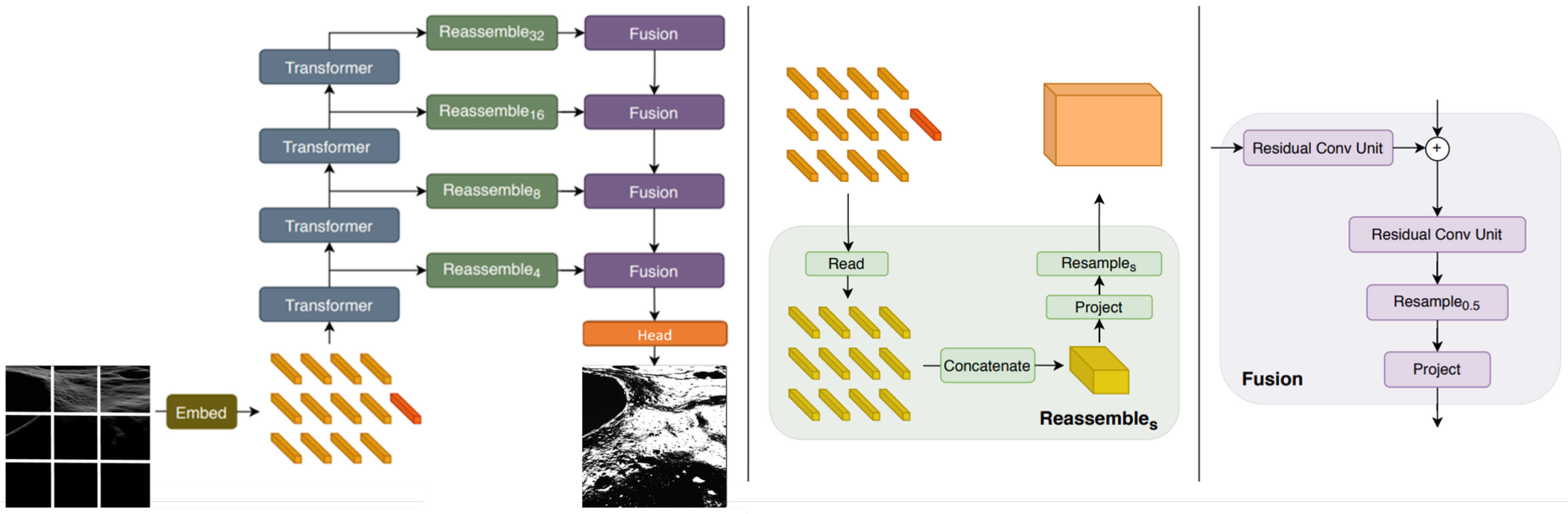
2.1. Architecture
- 1
- Compute scores , which measures the degree of attention of the surrounding image patches.
- 2
- Normalize the scores for the stability of the gradient
- 3
- Translate the scores into a probability with the softmax function
- 4
- Compute weighted value matrix
- Read block: this reads the input to be mapped into a representation size, by concatenating the readout token. The readout token is generally responsible for aggregating information from other tokens [30]. However, in the case of vision transformers, their performance is limited.
- Concatenate block: in this block, the representations are combined. The step consists of concatenating each representation following the order of the patches. This yields an image-like representation of this feature map.
- Resample block: This block consists of applying a 1 × 1 convolution to project the input image-like representation into a space of dimension 256. This convolutional block is followed by another 3 × 3 convolution to implement spatial downsampling and upsampling operations.where s is the chosen scale size of the representation.
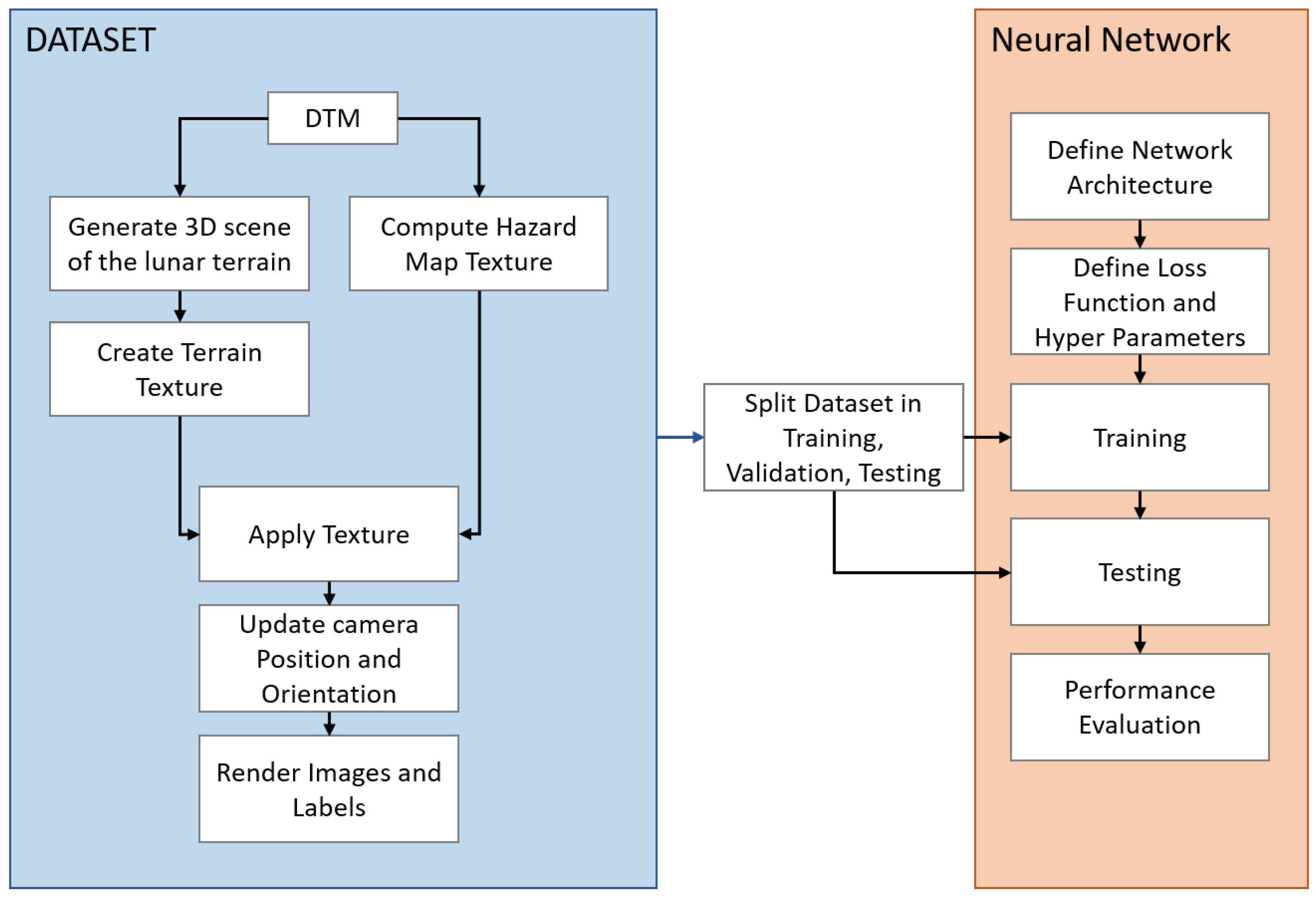
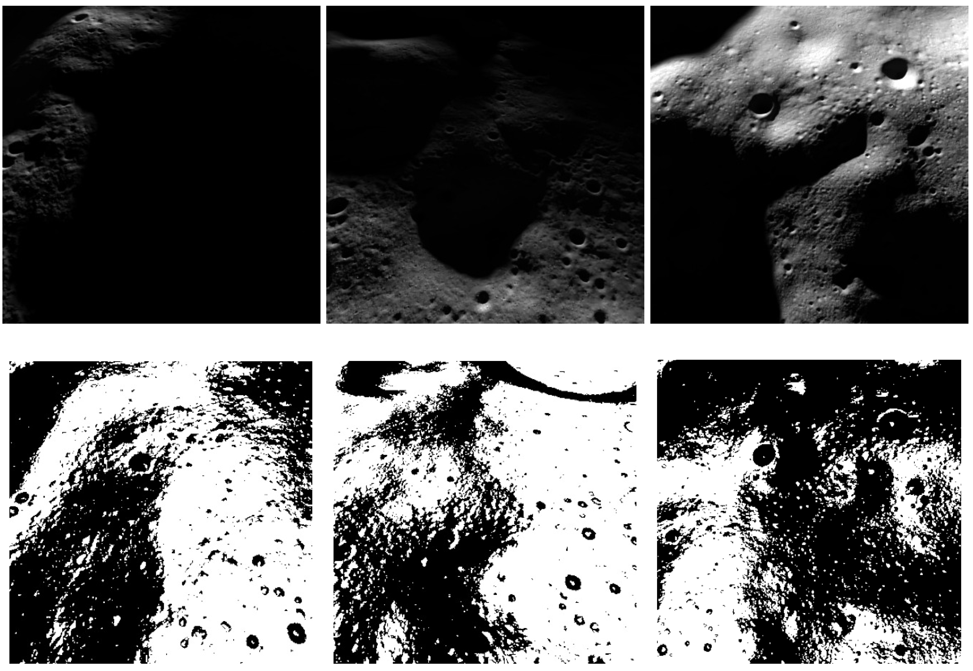
2.2. Dataset
3. Parameters
4. Metrics
- = true positive, data points predicted as hazardous that are hazardous.
- = true negative, data points predicted as safe that are safe.
- = false positive, data points predicted as hazardous that are safe.
- = false negative, data points predicted as safe that are hazardous.
4.1. Precision vs. Recall
4.2. Intersection over Union
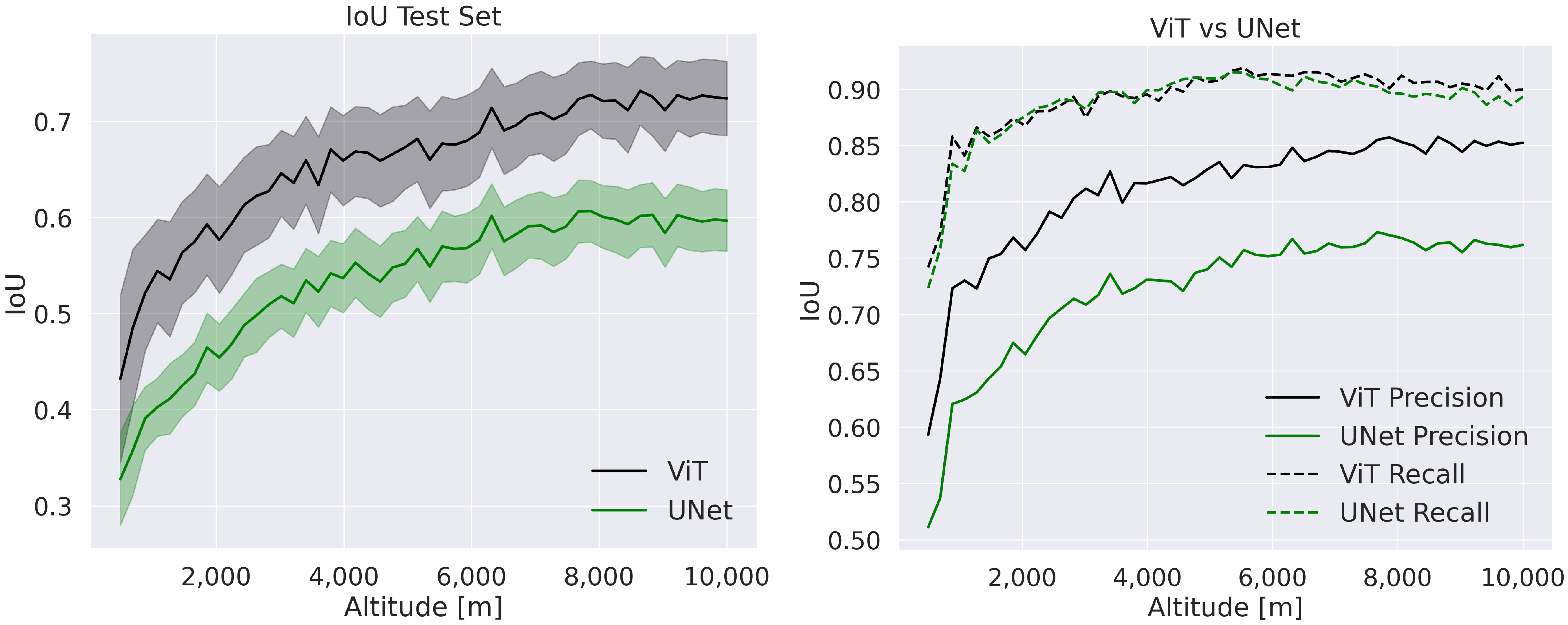
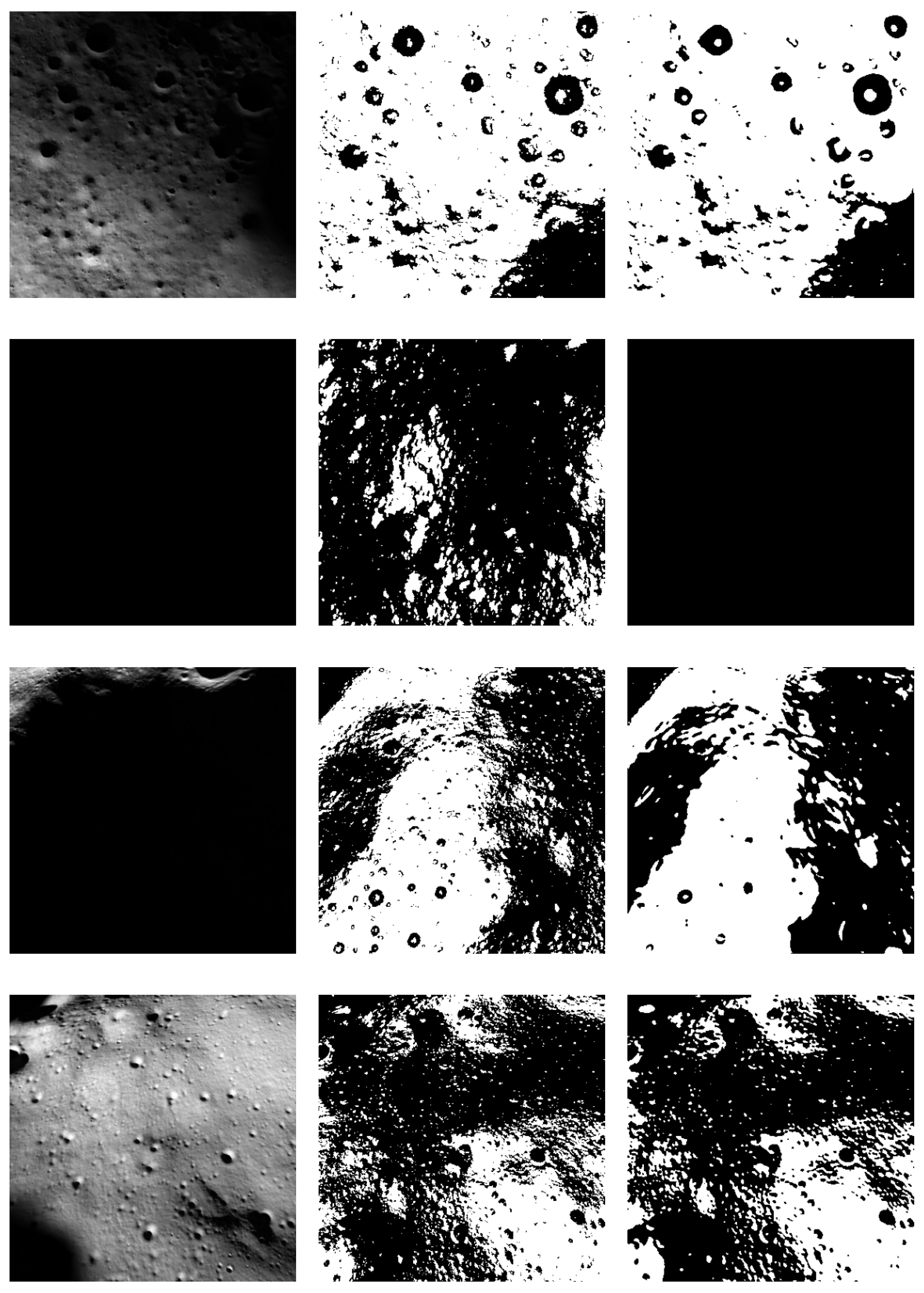
5. Results
6. Conclusions
Author Contributions
Funding
Institutional Review Board Statement
Informed Consent Statement
Data Availability Statement
Conflicts of Interest
Abbreviations
| Lidar | Light detection and ranging |
| ALHAT | Autonomous precision landing and hazard detection and avoidance technology |
| GNC | Guidance-navigation and control |
| DCE | Deep convolutional encode |
| NLP | Natural language processing |
| ViT | Vision transformer |
| DOF | Degrees of freedom |
| MHSA | Multihead self-attention |
| FFN | Feed-forward network |
| BSDF | Bidirectional scattering distribution function |
| DTM | Digital terrain model |
| TP | True positive |
| TN | True negative |
| FP | False positive |
| FN | False negative |
| IoU | Intersection over union |
References
- Epp, C.D.; Smith, T.B. Autonomous precision landing and hazard detection and avoidance technology (ALHAT). In Proceedings of the 2007 IEEE Aerospace Conference, Big Sky, MT, USA, 3–10 March 2007; pp. 1–7. [Google Scholar]
- Carson, J.M.; Trawny, N.; Robertson, E.; Roback, V.E.; Pierrottet, D.; Devolites, J.; Hart, J.; Estes, J.N. Preparation and integration of ALHAT precision landing technology for Morpheus flight testing. In Proceedings of the AIAA SPACE 2014 Conference and Exposition, San Diego, CA, USA, 4–7 August 2014; p. 4313. [Google Scholar]
- Epp, C.; Robertson, E.; Carson, J.M. Real-time hazard detection and avoidance demonstration for a planetary lander. In Proceedings of the AIAA SPACE 2014 Conference and Exposition, San Diego, CA, USA, 4–7 August 2014; p. 4313. [Google Scholar]
- Directorate, E.S.M. ESMD-RQ-0011 Preliminary (Rev. E) Exploration Crew Transportation System Requirements Document (Spiral 1); National Aeronautics and Space Administration: Washington, DC, USA, 2005; pp. 31–45.
- Wei, R.; Jiang, J.; Ruan, X.; Li, J. Landing Area Selection Based on Closed Environment Avoidance from a Single Image During Optical Coarse Hazard Detection. Earth Moon Planets 2018, 121, 73–104. [Google Scholar] [CrossRef]
- Li, S.; Jiang, X.; Tao, T. Guidance summary and assessment of the Chang’e-3 powered descent and landing. J. Spacecr. Rocket. 2016, 53, 258–277. [Google Scholar] [CrossRef]
- Zhang, H.; Li, J.; Wang, Z.; Guan, Y. Guidance navigation and control for Chang’E-5 powered descent. Space Sci. Technol. 2021, 2021, 9823609. [Google Scholar] [CrossRef]
- Zhang, H.; Guan, Y.; Cheng, M.; Li, J.; Yu, P.; Zhang, X.; Wang, H.; Yang, W.; Wang, Z.; Yu, J.; et al. Guidance navigation and control for Chang’E-4 lander. Sci. Sin. Technol. 2019, 49, 1418–1428. [Google Scholar]
- Canny, J. A computational approach to edge detection. IEEE Trans. Pattern Anal. Mach. Intell. 1986, PAMI-8, 679–698. [Google Scholar] [CrossRef]
- D’Ambrosio, A.; Carbone, A.; Spiller, D.; Curti, F. pso-based soft lunar landing with hazard avoidance: Analysis and experimentation. Aerospace 2021, 8, 195. [Google Scholar] [CrossRef]
- Vincent, O.R.; Folorunso, O. A descriptive algorithm for sobel image edge detection. In Proceedings of the Informing Science & IT Education Conference (InSITE), Macon, GE, USA, 12–15 June 2009; Informing Science Institute: Santa Rosa, CA, USA, 2009; Volume 40, pp. 97–107. [Google Scholar]
- Mokhtarian, F.; Suomela, R. Robust image corner detection through curvature scale space. IEEE Trans. Pattern Anal. Mach. Intell. 1998, 20, 1376–1381. [Google Scholar] [CrossRef]
- Harris, C.G.; Stephens, M. A combined corner and edge detector. In Proceedings of the Alvey Vision Conference, Citeseer, Manchester, UK, 31 August 1988; Volume 15, pp. 10–5244. [Google Scholar]
- Mahmood, W.; Shah, S.M.A. Vision based hazard detection and obstacle avoidance for planetary landing. In Proceedings of the 2009 2nd International Workshop on Nonlinear Dynamics and Synchronization, Klagenfurt, Austria, 20–21 July 2009; pp. 175–181. [Google Scholar]
- Lunghi, P.; Ciarambino, M.; Lavagna, M. A multilayer perceptron hazard detector for vision-based autonomous planetary landing. Adv. Astronaut. Sci. 2016, 156, 1717–1734. [Google Scholar] [CrossRef]
- Li, X.; Chen, H.; Qi, X.; Dou, Q.; Fu, C.W.; Heng, P.A. H-DenseUNet: Hybrid densely connected UNet for liver and tumor segmentation from CT volumes. IEEE Trans. Med. Imaging 2018, 37, 2663–2674. [Google Scholar] [CrossRef] [PubMed]
- Ghilardi, L.; D’Ambrosio, A.; Scorsoglio, A.; Furfaro, R.; Curti, F. Image-based lunar landing hazard detection via deep learning. In Proceedings of the 31st AAS/AIAA Space Flight Mechanics Meeting, Virtual, 31 January–4 February 2021; pp. 1–4. [Google Scholar]
- Scorsoglio, A.; D’Ambrosio, A.; Ghilardi, L.; Furfaro, R.; Gaudet, B.; Linares, R.; Curti, F. Safe Lunar landing via images: A Reinforcement Meta-Learning application to autonomous hazard avoidance and landing. In Proceedings of the 2020 AAS/AIAA Astrodynamics Specialist Conference, Virtual, 9–13 August 2020; pp. 9–12. [Google Scholar]
- Moghe, R.; Zanetti, R. A Deep learning approach to Hazard detection for Autonomous Lunar landing. J. Astronaut. Sci. 2020, 67, 1811–1830. [Google Scholar] [CrossRef]
- Ronneberger, O.; Fischer, P.; Brox, T. U-net: Convolutional networks for biomedical image segmentation. In Proceedings of the International Conference on Medical Image Computing and Computer-Assisted Intervention, Munich, Germany, 5–9 October 2015; pp. 234–241. [Google Scholar]
- Downes, L.; Steiner, T.J.; How, J.P. Deep Learning Crater Detection for Lunar Terrain Relative Navigation. In Proceedings of the AIAA Scitech 2020 Forum, Orlando, FL, USA, 6–10 January 2020; p. 1838. [Google Scholar]
- Pugliatti, M.; Maestrini, M. Small-body segmentation based on morphological features with a u-shaped network architecture. J. Spacecr. Rocket. 2022, 59, 1821–1835. [Google Scholar] [CrossRef]
- Vaswani, A.; Shazeer, N.; Parmar, N.; Uszkoreit, J.; Jones, L.; Gomez, A.N.; Kaiser, Ł.; Polosukhin, I. Attention is all you need. Adv. Neural Inf. Process. Syst. 2017, 30, 5998–6008. [Google Scholar]
- Dosovitskiy, A.; Beyer, L.; Kolesnikov, A.; Weissenborn, D.; Zhai, X.; Unterthiner, T.; Dehghani, M.; Minderer, M.; Heigold, G.; Gelly, S.; et al. An image is worth 16x16 words: Transformers for image recognition at scale. arXiv 2020, arXiv:2010.11929. [Google Scholar]
- Ghilardi, L.; Scorsoglio, A.; Furfaro, R. ISS Monocular Depth Estimation Via Vision Transformer. In Proceedings of the International Conference on Applied Intelligence and Informatics, Reggio Calabria, Italy, 1–3 September 2022; pp. 167–181. [Google Scholar]
- Ranftl, R.; Bochkovskiy, A.; Koltun, V. Vision transformers for dense prediction. In Proceedings of the IEEE/CVF International Conference on Computer Vision, Montreal, BC, Canada, 10–17 October 2021; pp. 12179–12188. [Google Scholar]
- Jiang, K.; Peng, P.; Lian, Y.; Xu, W. The encoding method of position embeddings in vision transformer. J. Vis. Commun. Image Represent. 2022, 89, 103664. [Google Scholar] [CrossRef]
- Khan, S.; Naseer, M.; Hayat, M.; Zamir, S.W.; Khan, F.S.; Shah, M. Transformers in vision: A survey. ACM Comput. Surv. (CSUR) 2022, 54, 1–41. [Google Scholar] [CrossRef]
- Deng, J.; Dong, W.; Socher, R.; Li, L.J.; Li, K.; Fei-Fei, L. Imagenet: A large-scale hierarchical image database. In Proceedings of the 2009 IEEE Conference on Computer Vision and Pattern Recognition, Miami, FL, USA, 20–25 June 2009; pp. 248–255. [Google Scholar]
- Lo, C.C.; Vandewalle, P. RCDPT: Radar-Camera Fusion Dense Prediction Transformer. In Proceedings of the ICASSP 2023–2023 IEEE International Conference on Acoustics, Speech and Signal Processing (ICASSP), Rhodes Island, Greece, 4–10 June 2023; pp. 1–5. [Google Scholar]
- Barker, M.K.; Mazarico, E.; Neumann, G.A.; Smith, D.E.; Zuber, M.T.; Head, J.W. Improved LOLA elevation maps for south pole landing sites: Error estimates and their impact on illumination conditions. Planet. Space Sci. 2021, 203, 105119. [Google Scholar] [CrossRef]
- Mazarico, E.; Neumann, G.; Smith, D.; Zuber, M.; Torrence, M. Illumination conditions of the lunar polar regions using LOLA topography. Icarus 2011, 211, 1066–1081. [Google Scholar] [CrossRef]
- Boncelet, C. Image noise models. In The Essential Guide to Image Processing; Elsevier: Amsterdam, The Netherlands, 2009; pp. 143–167. [Google Scholar]
- Penttilä, A.; Palos, M.F.; Kohout, T. Realistic visualization of solar system small bodies using Blender ray tracing software. In Proceedings of the European Planetary Science Congress, Virtual, 13–24 September 2021; p. EPSC2021-791. [Google Scholar]
- Golish, D.; DellaGiustina, D.; Li, J.Y.; Clark, B.; Zou, X.D.; Smith, P.; Rizos, J.; Hasselmann, P.; Bennett, C.; Fornasier, S.; et al. Disk-resolved photometric modeling and properties of asteroid (101955) Bennu. Icarus 2021, 357, 113724. [Google Scholar] [CrossRef]


| Blocks | Channels |
|---|---|
| Double Conv. | 3 → 64 |
| Down1 | 64 → 128 |
| Down2 | 128 → 256 |
| Down3 | 256 → 512 |
| Down4 | 512 → 1024 |
| Up1 | 1024 → 512 |
| Up2 | 512 → 256 |
| Up3 | 256 → 128 |
| Up4 | 128 → 64 |
| Classification Head | 64 → 2 |
| Blocks | Layers |
| Double Conv. | Conv2D |
| BatchNorm2D | |
| ReLU | |
| Conv2D | |
| BatchNorm2D | |
| ReLU | |
| Down | MaxPool2D |
| Double Conv. | |
| Up | Bilinear Up-Sampling |
| Double Conv. | |
| Classification Head | Conv2D |
Disclaimer/Publisher’s Note: The statements, opinions and data contained in all publications are solely those of the individual author(s) and contributor(s) and not of MDPI and/or the editor(s). MDPI and/or the editor(s) disclaim responsibility for any injury to people or property resulting from any ideas, methods, instructions or products referred to in the content. |
© 2023 by the authors. Licensee MDPI, Basel, Switzerland. This article is an open access article distributed under the terms and conditions of the Creative Commons Attribution (CC BY) license (https://creativecommons.org/licenses/by/4.0/).
Share and Cite
Ghilardi, L.; Furfaro, R. Image-Based Lunar Hazard Detection in Low Illumination Simulated Conditions via Vision Transformers. Sensors 2023, 23, 7844. https://doi.org/10.3390/s23187844
Ghilardi L, Furfaro R. Image-Based Lunar Hazard Detection in Low Illumination Simulated Conditions via Vision Transformers. Sensors. 2023; 23(18):7844. https://doi.org/10.3390/s23187844
Chicago/Turabian StyleGhilardi, Luca, and Roberto Furfaro. 2023. "Image-Based Lunar Hazard Detection in Low Illumination Simulated Conditions via Vision Transformers" Sensors 23, no. 18: 7844. https://doi.org/10.3390/s23187844
APA StyleGhilardi, L., & Furfaro, R. (2023). Image-Based Lunar Hazard Detection in Low Illumination Simulated Conditions via Vision Transformers. Sensors, 23(18), 7844. https://doi.org/10.3390/s23187844