1. Introduction
Remote sensing imagery is widely used in various fields, such as geological exploration, urban planning, and environmental monitoring. However, various noise sources, such as circuit noise and dark current noise [
1], can introduce Gaussian noise into remote sensing imagery. In addition, noise interference during digital image transmissions and storage can result in salt-and-pepper noise. These noise sources degrade image quality, affecting subsequent analyses and applications [
2]. Therefore, denoising is crucial for processing remote sensing images.
Denoising methods for remote sensing images typically employ linear or nonlinear filtering techniques, such as median filtering [
3], Gaussian filtering [
4], or a wavelet transform [
5]. However, these methods have certain limitations. For instance, median filtering can result in image distortion [
6], and a wavelet transform involves complex decomposition and reconstruction operations [
7]. The bilateral filter, proposed by Tomasi and Mandeville [
8] in the 1980s, has undergone improvements and developments and has emerged as a suitable method for image denoising and edge preservation. Chen et al. [
9] proposed a denoising approach by combining a wavelet transform and bilateral filtering. They utilized multilevel thresholding based on a wavelet analysis to handle mixed noise and effectively eliminate noise at different frequencies in the image. Deng et al. [
10] integrated adaptive parameter bilateral filtering with a wavelet transform to improve image retrieval. They used the Corel-5K image database for validation and achieved a high applicability. Lin [
11] proposed the concept of gradient similarity to distinguish between edge blocks and non-edge blocks in image processing and improved bilateral filtering by employing gradient similarity instead of grayscale similarity. Zhang et al. [
12] developed a novel two-step denoising method for handling mixed noise. They employed the DnCNN denoising model to reduce Gaussian noise and used an adaptive median filtering technique to reduce salt-and-pepper noise. Liu et al. [
13] proposed an adaptive median filter with edge preservation wherein the edge is first extracted using an edge extractor, and then the median-filtered image is fused with the extracted edge to realize effective filtering and edge enhancement.
Bilateral filtering represents an extended form of the Gaussian filtering methodology. This technique incorporates two key factors during image processing: the spatial coordinates of pixels and the disparities in pixel intensities. This amalgamation enables the enhanced preservation of edge data [
14]. In contrast, conventional Gaussian filtering exclusively addresses the spatial arrangement of pixels by employing a Gaussian kernel to execute the weighted averaging of neighboring pixels, thereby facilitating a resultant blurring outcome. Notably, the inherent limitation of conventional Gaussian filtering resides in its omission of intensity discrepancies among pixels. The advent of bilateral filtering introduces an additional layer of weighting within the intensity domain, superimposed upon the principles of Gaussian filtering. This approach not only considers the spatial separation between pixels, but also takes into careful consideration the disparities in pixel intensities. As a result, bilateral filtering achieves a dual objective: the retention of edge information alongside the realization of smoothing effects.
In this paper, we proposed a remote sensing image denoising method based on multi-objective optimized bilateral filtering. The proposed method employs several techniques to enhance the bilateral filtering parameters. It combines edge detection operators and the differential evolution (DE) algorithm with traditional bilateral filtering. The adjusted parameters include the convolution kernel size, the spatial standard deviation of pixel positions, and the color space standard deviation of pixel values. These modifications greatly improve the noise reduction capabilities of the proposed method. Furthermore, the implementation process and experimental results of the proposed method are discussed in this paper. The results demonstrated a substantial enhancement in denoising performance while preserving the edges, thus indicating that the proposed method is suitable for subsequent processing and applications of remote sensing images.
2. Principles and Methods of Filtering Algorithms
2.1. Bilateral Filtering
Bilateral filtering is a powerful nonlinear filtering method that eliminates noise and preserves edge details in an image. It is based on a weighted average of the image’s spatial domain and grayscale value domain. The weights are determined based on the product of a spatial domain Gaussian kernel and a grayscale value domain Gaussian kernel [
15,
16]. By considering the spatial distance between pixels and the disparity in grayscale values, bilateral filtering assigns appropriate weights, resulting in the improved preservation of edges and fine details. The formula for bilateral filtering is as follows:
where
represents the spatial domain Gaussian kernel,
denotes the grayscale value domain Gaussian kernel,
is the weight,
is the spatial distance between pixels (the Euclidean distance between pixels in an image),
denotes the color difference between pixels
and
,
is the spatial standard deviation, and
is the color space standard deviation.
2.2. Canny Operator
The Canny edge detection algorithm is a multistage edge detection algorithm proposed by John F. Canny in 1986. This algorithm processes single-channel grayscale images by detecting the first and second derivatives of pixel intensities and determines whether a pixel is located on an edge [
17,
18].
The algorithm involves the following steps. Gaussian filtering is applied to the input grayscale image to effectively remove noise:
where (
x,
y) denote the coordinates of the filter and
σ denotes the standard deviation of the Gaussian function.
Next, the gradient magnitude and direction are computed for each pixel in the image:
Subsequently, non-maximum suppression is applied to the gradient magnitude to reduce the width of the detected edges.
The gradient magnitude is categorized into three groups by using a dual threshold algorithm: strong edges, weak edges, and non-edge pixels. Strong edges have gradient magnitudes surpassing the high threshold, weak edges have gradient magnitudes falling between the low and high thresholds, and non-edge pixels have gradient magnitudes below the low threshold. Furthermore, edge connectivity processing is employed for the weak edges to detect weak edge pixels adjacent to strong edges and upgrade their classification to strong edges. The integration process establishes connections among the weak edges, resulting in a comprehensive and refined edge detection outcome.
To determine the upper and lower thresholds for the Canny algorithm, an automated technique known as the Otsu method is applied. This method serves to establish the binarization threshold of the image, a crucial step in the process of image binarization segmentation. The Otsu method autonomously identifies a suitable threshold for binarization, thereby enabling the clear extraction of target object contours [
19,
20]. The Otsu algorithm’s core steps encompass the following:
The image’s histogram is computed, tabulating the occurrences of grayscale levels for each pixel.
The within-class variance is calculated by categorizing pixels into two groups, namely the background and the foreground, based on each possible threshold value “
t”. The between-class variance
is calculated for each “
t” according to the formula:
Here, “k” signifies the two categories 0 and 1; “ω” denotes the proportion of pixels with grayscale values less than or equal to “t” in the “k”-th class; and represents the average grayscale value of pixels with grayscale values less than or equal to “t” in the “k”-th class.
The global inter-class variance
is calculated.
The optimal threshold is identified by selecting from all feasible thresholds the one that maximizes the inter-class variance g(t). By undergoing this computation, the Otsu algorithm automatically pinpoints the most appropriate binarization threshold, thereby enhancing the distinction between the foreground and the background and effectively facilitating object extraction from the image. In this study, the high and low thresholds for the Canny algorithm utilize binarization thresholds determined by the Otsu algorithm, scaled by 0.5 and 1.5 times.
2.3. Differential Evolution Algorithm
The DE algorithm is an optimization algorithm primarily used to solve multidimensional continuous optimization problems. It was proposed by Storn and Price in 1997 and has since become a widely used global optimization algorithm [
21,
22,
23]. The fundamental concept of the DE algorithm is to iteratively improve a population of individuals by manipulating their differences. Through this iterative process, a new population is created, and the individuals within the population are progressively optimized. The DE algorithm mainly comprises the following steps:
First, an initial population, where each individual represents a potential solution, is randomly generated:
where
1, 2, 3, …,
NP (population size);
1, 2, 3, …,
D (dimensionality); and
denotes a uniformly distributed random number in the interval [0, 1].
The mutation operation randomly selects three distinct individuals and updates the current individual’s position by using the difference vectors between them, resulting in a new candidate solution:
where
, and
are distinct integers selected from the interval [1,
NP].
During the crossover operation, the mutation vector is combined with the original individual to create a new individual. The target vector
is crossed with the mutation vector
to create the trial vector
:
where
is a random integer selected from the range [1, D] to ensure that
carries information. The crossover probability
has a value between 0 and 1.
The selection operation involves comparing the trial individuals with the original individuals and selecting the superior individuals as members of the next-generation population:
where
represents the objective function.
The termination criteria for the DE algorithm are met when either the maximum predetermined number of generations is reached or when the objective function has converged to a considerable extent. At this stage, the algorithm concludes and outputs the optimal solution.
3. Multiscale-Optimized Bilateral Filtering
The parameters of the bilateral filter, such as the spatial domain filter kernel and the standard deviation of the spatial domain Gaussian kernel, are adjusted using the Canny operator. First, the Otsu thresholding technique is used to adjust the high and low thresholds (
and
, respectively) of the Canny edge detection operator:
Strong edge pixels of an edge response are defined as , weak edge pixels of an edge response are defined as , and non-edge pixels are defined as .
The edge width is computed using non-maximum suppression:
The standard deviation of the edge response image is computed as follows:
where
µ denotes the population mean and
xi represents the
i-th sample data point.
The spatial domain Gaussian kernel
is optimized:
where
and
are the coordinates of pixel points
and
, respectively, and
is replaced by
(the standard deviation of the edge response image).
The spatial domain filter kernel
D is optimized:
where
is the edge width and
σ is the standard deviation of the edge response image.
The pixel range domain kernel
is optimized by using the DE algorithm:
where
denotes the color difference (calculated using the Euclidean distance) between pixels
and
and
denotes the standard deviation of the color space of the pixel values:
A population of 20 individuals is randomly generated within the range of [
σ, 2
σ] and their parameter vectors are initialized. The crossover probability, mutation probability, and number of iterations are set as 0.5, 0.1, and 400, respectively. The fitness function peak signal-to-noise ratio (PSNR) is defined to assess the fitness of each individual by determining the PSNR value of the filtered image corresponding to each individual:
where
represents the PSNR function.
Individuals with a better fitness are selected from the population, and genetic operators such as crossover and mutation operations are applied to them to generate new individuals. The population is then updated by replacing the individuals with the newly generated ones. This is constantly iterated, ultimately yielding the optimal parameters and their respective PSNR values.
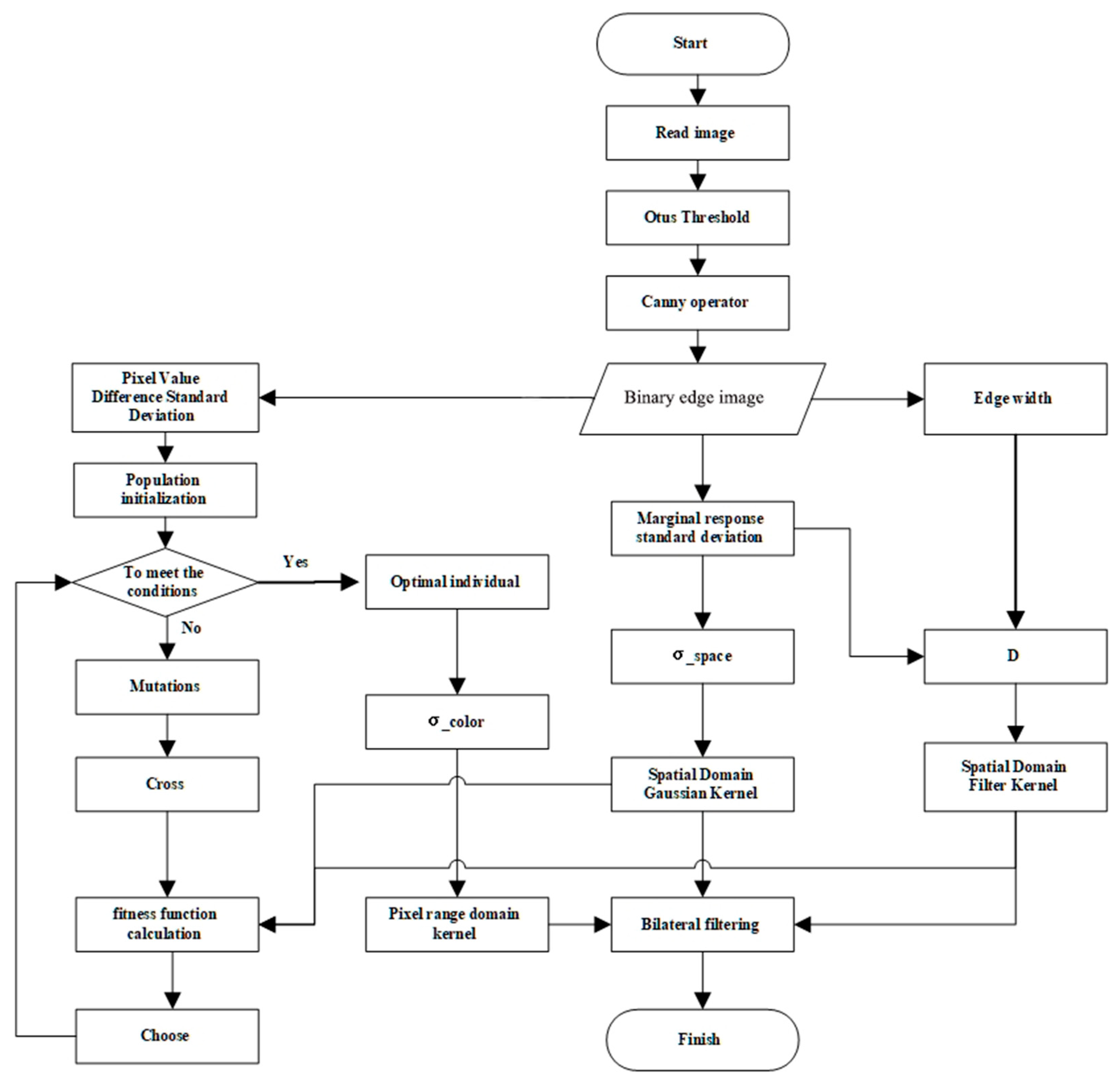
The flowchart of the multiscale-optimized bilateral filtering algorithm is illustrated in
Figure 1.
Multiscale-optimized bilateral filtering offers several advantages. It adjusts the spatial domain Gaussian kernel and spatial domain filter kernel (D is the convolution kernel size) of the bilateral filtering based on the standard deviation and the edge response width of the Canny operator; moreover, it employs the DE algorithm to optimize the pixel range domain kernel. The advantages are listed as follows:
Edge preservation and smoothness control: The standard deviation of the Canny operator indicates the intensity variation in the edges of the image. By adjusting the size of the spatial domain Gaussian kernel based on the standard deviation of the Canny operator, the smoothness of the filter can be controlled. When the standard deviation of the Canny operator is larger, increasing the size of the spatial domain Gaussian kernel enhances the smoothing effect. In contrast, when the standard deviation of the Canny operator is smaller, reducing the size of the spatial domain Gaussian kernel helps preserve more details during the filtering process.
Noise suppression: The convolution kernel size (D) of bilateral filtering can be used to control the degree of noise suppression. A larger convolution kernel can effectively average the neighboring pixel values and reduce the effect of noise. By dynamically adjusting the convolution kernel size based on the standard deviation and edge response width of the Canny operator, an optimal kernel size that aligns with the intensity of the noise can be adaptively selected, enabling superior noise suppression.
High adaptability: The DE algorithm, which incorporates differential and mutation operations, enables a global search and the automatic selection of the optimal standard deviation for the pixel value color space based on the characteristics of the image. By considering the characteristics of the image, the DE algorithm selects the optimal standard deviation for the pixel value color space to adjust the pixel range domain kernel. This is achieved by combining it with the spatial domain Gaussian kernel and kernel size, enabling adaptive filtering.
4. Evaluation Criteria
4.1. Mean Squared Error
The mean squared error (
MSE) is a commonly used metric for evaluating the denoising performance of image-processing algorithms. It is the average of the squared differences between the image pixel values and their corresponding true values. A smaller
MSE indicates a more effective denoising result [
24]:
where
I and
J represent images of the same size with a width
W and a height
H, and
and
denote their pixel values, respectively.
The
PSNR is a metric used for evaluating image quality [
25]. It quantifies the ratio between the signal and the noise by using the maximum possible signal value as a reference. The
PSNR is commonly used to compare the disparity in quality between an image and its post-processed version, such as after compression or denoising. The calculation formula for the
PSNR is as follows:
4.2. Structural Similarity Index
The structural similarity index (
SSIM) is a standardized metric used for measuring the degree of similarity between two images. Unlike conventional metrics such as the
MSE and
PSNR, the
SSIM better corresponds to the human visual perception of image quality [
26]. It considers three aspects: luminance, contrast, and structure. The
SSIM compares the mean, variance, and covariance of the pixel values in the two images, and these metrics are then weighted and aggregated to obtain the final similarity score.
SSIM values range from −1 to 1, with a higher value indicating a stronger similarity between two images. An
SSIM value of 1 means that the two images are perfectly identical.
where
and
denote the mean values of images x and y, respectively;
and
are the standard deviations of the pixel values in images
x and
y, respectively;
denotes the covariance of the pixel values; and
and
are two constants introduced to avoid potential errors resulting from excessively small denominators that may lead to division by zero.
5. Experiment and Analysis
In this study, we conducted a remote sensing image denoising simulation experiment by using DF-1 satellite images and drone orthophotos with dimensions of 600 × 600 and 472 × 502 pixels, respectively. Gaussian noise was added to the images at four different concentration levels: 1%, 2%, 3%, and 4%. Subsequently, denoising experiments were performed, and the results were analyzed both qualitatively and quantitatively. A comparison of the denoising effectiveness of the multiple-optimization bilateral filtering (MOBF) algorithm and several other denoising techniques, namely anisotropic filtering (AF), adaptive median filtering (AMF), original bilateral filtering (BF), wavelet denoising (WD), and non-local means (NLM), was performed. The denoised images were evaluated using objective metrics such as the PSNR, the MSE, and the SSIM. Furthermore, an analysis of the noise power spectral density was conducted to determine the level of information preservation across different frequency domains, thus providing valuable insights into the effectiveness of the denoising techniques.
In order to find the optimal parameters of the DE algorithm, this paper conducts experiments under the conditions of a Gaussian noise concentration of 1% or 3%, and changes the iterative parameters of the DE algorithm to find the optimal parameters. The parameter of the iteration with the largest noise ratio (PSNR) is obtained through experiments. The optimal number of iterations is 400. Therefore, the number of iterations of the DE algorithm in the remote sensing simulation experiment in this paper is set to 400. The figure below shows the process of parameter optimization. The experimental results are shown in
Figure 2.
5.1. GF-1 Image Simulation Experiment
To validate the effectiveness of the proposed denoising algorithm, an experiment was conducted using GF-1 imagery for a remote sensing image simulation. A higher PSNR value indicated superior denoising results, reflecting a closer resemblance between the processed and original images. A smaller MSE value indicated a higher level of similarity in pixel values between the processed and original images, indicating minimal distortion. A higher SSIM value indicated an improved performance in terms of human perception, encompassing factors such as the brightness, contrast, and structural fidelity. The experimental results are presented in
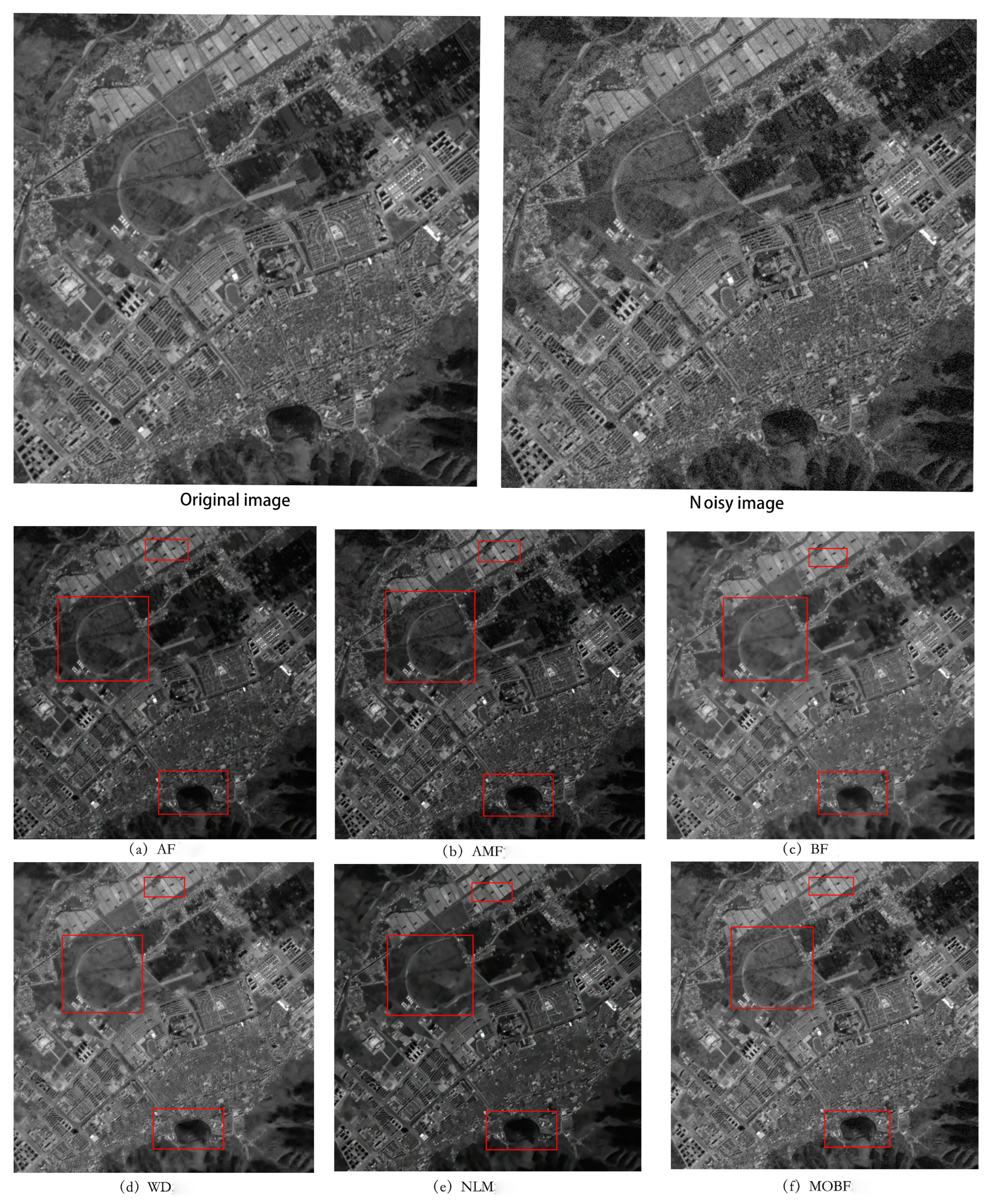
Table 1, and a denoising comparison of GF-1 images with a noise concentration of 4% is shown in
Figure 3.
As can be seen from
Figure 3, the MOBF algorithm outperformed other methods in terms of the denoising performance on GF-1 images. Notably, as can be seen in
Figure 3f, the preserved texture details within the rectangular box region were visually more prominent than those obtained using other algorithms. Furthermore, as can be observed from the data presented in
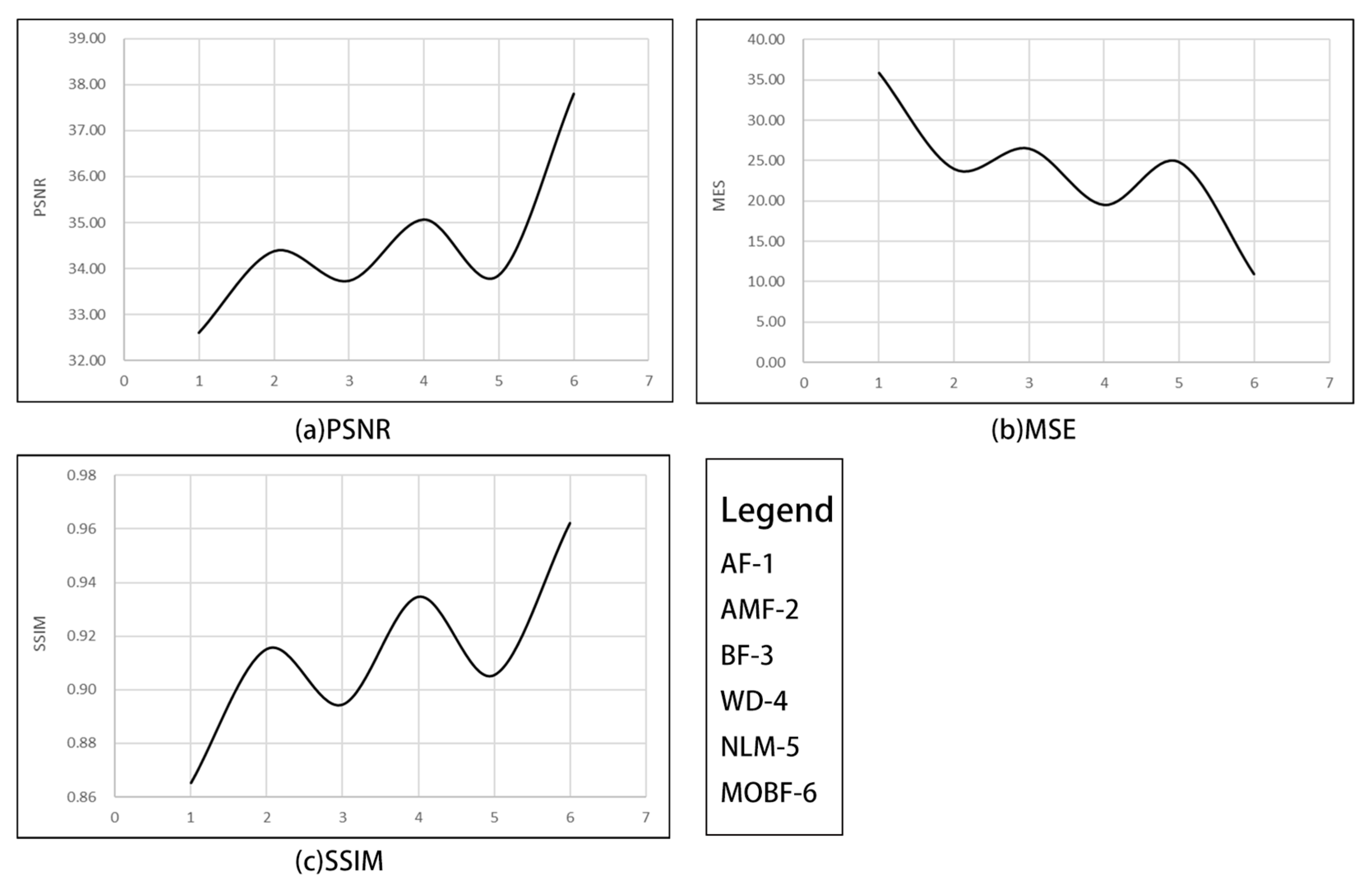
Table 1, the MOBF algorithm achieved the highest PSNR and SSIM values and the lowest MSE value across images with different noise densities. The algorithm performance is shown in
Figure 4.
5.2. Unmanned Aerial Vehicle Image Simulation Experiment
Similarly, a simulation experiment was conducted on unmanned aerial vehicle (UAV) remote sensing images to assess the denoising effectiveness of different algorithms in terms of three metrics: the PSNR, the MSE, and the SSIM. The experiment’s results are presented in
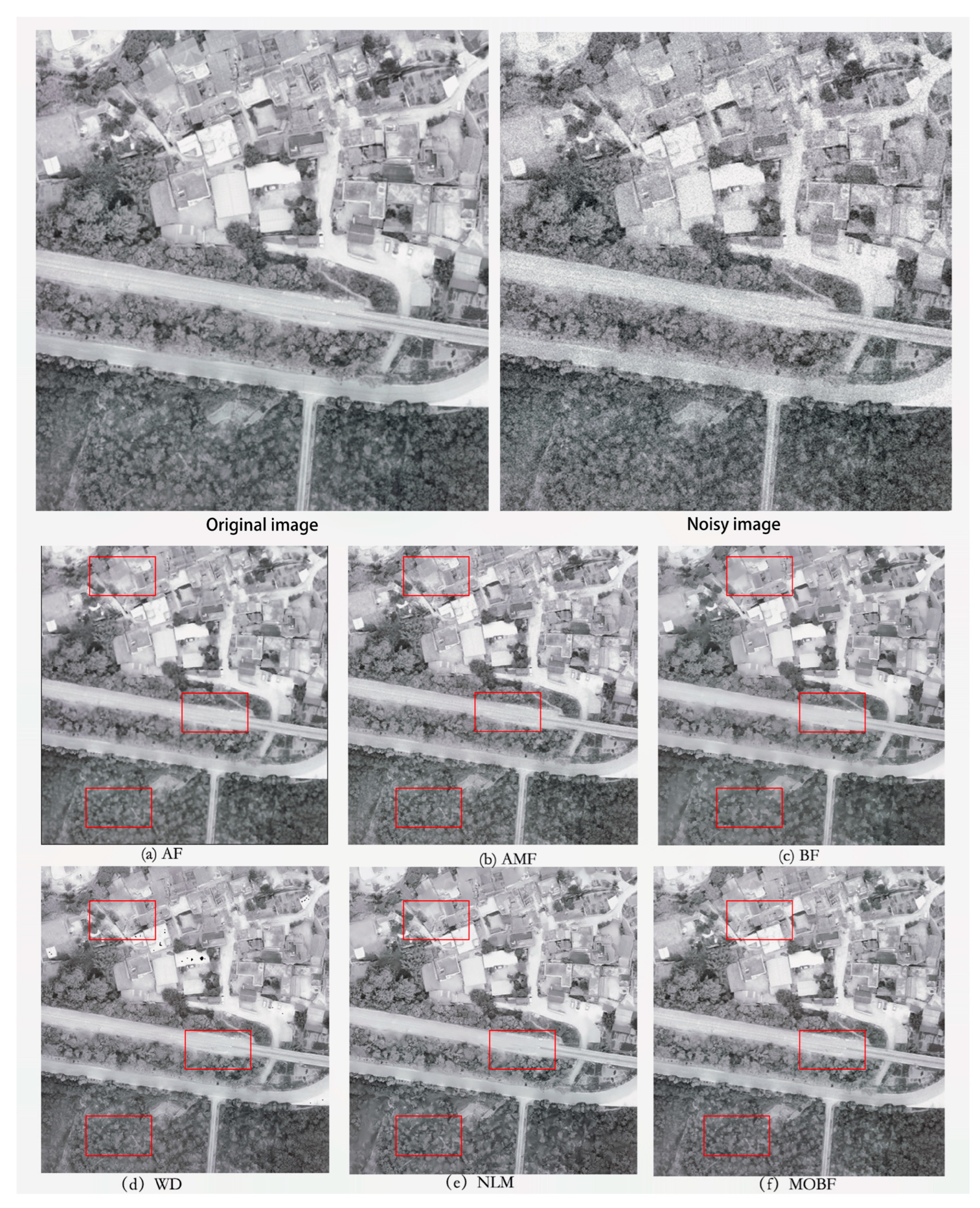
Table 2, and a comparative visualization of the denoising outcomes for UAV images is displayed in
Figure 5.
As can be seen in
Figure 4, the AF, AMF, BF, WD, and NLM algorithms exhibited a considerably higher level of the smoothing effect within the rectangular box region after denoising, surpassing the performance of the MOBF algorithm. However, these algorithms sacrificed some texture details in the process. A further analysis and comparison of the BF and MOBF algorithms revealed that optimized bilateral filtering excels at preserving the edge details of building rooftops, roads, and vegetation areas. A comparison of the BF and MOBF algorithms is shown in
Figure 6.
As can be observed from the experimental results summarized in
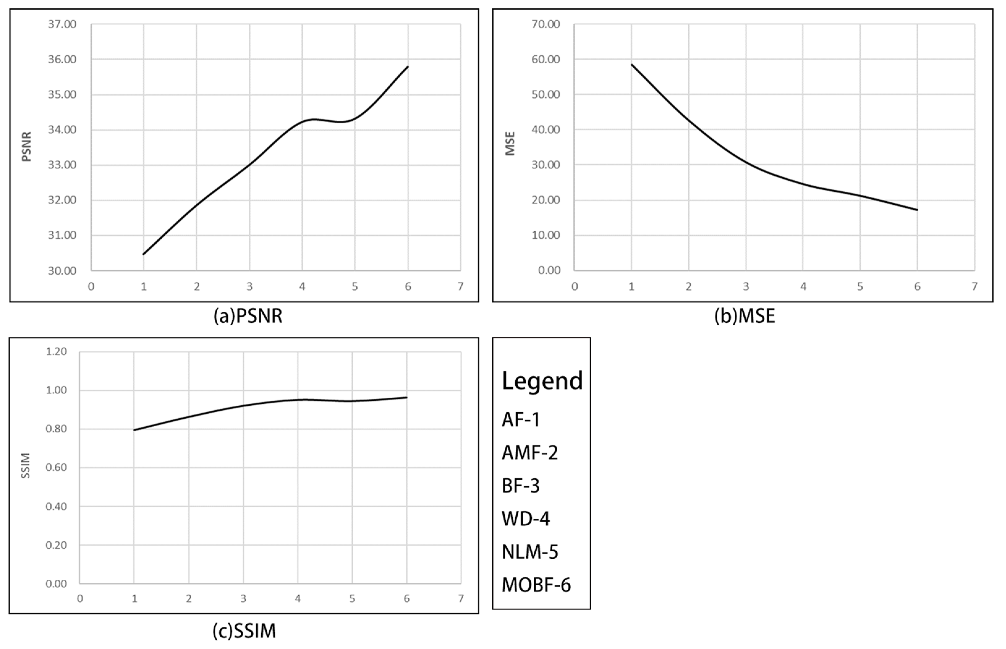
Table 2, the proposed MOBF algorithm outperformed the traditional BF, WD, and NLM algorithms for all three evaluation metrics, thus demonstrating that the remote sensing images processed using the MOBF algorithm exhibit an improved denoising performance and enhanced edge preservation. The algorithm performance is shown in
Figure 7.
In the power spectral density (PSD) plot of an image, the low-frequency region corresponds to low-frequency information, the overall brightness, and the color; the mid-frequency region represents texture information, details, textures, and other intricate patterns within the image; and the high-frequency region reveals edge information, including the edges, contours, and other distinct features within the image.
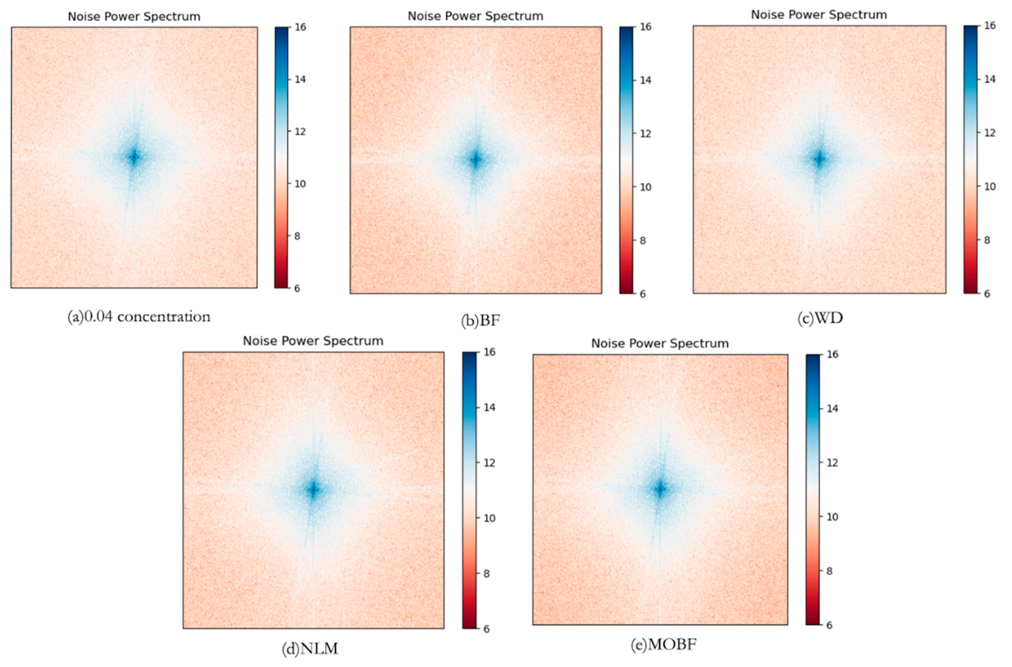
In this study, a comparison of noise power spectral density was performed between the proposed algorithm and three filtering algorithms (BF, WD, and NLM). The power spectral density plots of the images after applying different processing methods are shown in
Figure 8. The analysis of the power spectral density revealed that the information content in the low-, mid-, and high-frequency domains of the remote sensing images processed using the MOBF method was highly similar, thus indicating that the image modification did not result in a significant degradation of the texture, detail, or edge information. In the comparison of the MOBF algorithm with the BF algorithm, the higher energy of the MOBF algorithm in the mid-frequency region indicated better texture information preservation. In the comparison of the MOBF algorithm with the WD algorithm, the high-frequency region of the WD algorithm exhibited higher energy levels, exceeding even those of the original image, indicating that some noise remained uneliminated. The MOBF algorithm exhibited a higher energy level in the edge region compared to the NLM algorithm, thus demonstrating its superior edge preservation capability.
In the noise power spectral density plot, a high energy in the high-frequency region indicates the existence of high-frequency noise in the image, a high energy in the mid-frequency region indicates a considerable amount of detail and a lower level of image smoothness, and a higher energy in the low-frequency region is indicative of increased brightness and contrast in the image, leading to an overall brighter appearance. As can be observed from
Figure 8, the denoising effectiveness was in the following order: MOBF algorithm > BF algorithm > NLM algorithm > WD algorithm.
6. Conclusions
In this paper, the MOBF algorithm was proposed to improve upon traditional bilateral filtering in terms of denoising effectiveness and edge texture preservation by utilizing edge detection operators and the DE evolutionary algorithm for multiple optimizations. The optimizations are made at the spatial domain filter kernel, spatial domain Gaussian kernel, and pixel range domain kernel. The proposed MOBF algorithm exhibited satisfactory performance, even in the absence of input parameters for the bilateral filtering algorithm.
The experiments detailed in this paper focus on varying levels of Gaussian noise intensity. The denoising experimental results for remote sensing images demonstrated the superior performance of the MOBF algorithm. Evaluation metrics such as the PSNR, the MSE, and the SSIM revealed the superiority of the MOBF algorithm over traditional approaches. Based on the outcomes of the experiments, the algorithm introduced in this study demonstrates enhancements in comparison to the optimal outcomes achieved by the comparative algorithms. Notably, there was a noteworthy 2.79% enhancement in the PSNR, a substantial 6.25% decrease in the MSE, and a discernible 1.05% improvement in the SSIM. The images processed using the MOBF algorithm exhibited remarkable denoising and edge preservation effects, resulting in enhanced image clarity.
These results validate the feasibility and effectiveness of the MOBF algorithm for denoising remote sensing images. Future research can further explore the algorithm’s applicability in other remote sensing scenarios and focus on enhancing its computational efficiency and practicality to drive advancements in the field of remote sensing image processing.
Author Contributions
X.F. was responsible for the experimental design and data collection of this research. He participated in tasks such as noise simulation, image processing, and comparative experiments, providing reliable foundational data and the results for the experiments. Y.L. was the primary author of this paper, and was responsible for the overall structure and content writing. She also participated in some experimental work, conducted an in-depth analysis, and was responsible for the discussions on the methods and results presented in the paper. X.Z. made significant contributions to the algorithm and model design. He proposed the key denoising algorithm used in this study and conducted a relevant theoretical analysis. Additionally, X.Z. assisted in writing the methodology section. J.H. conducted extensive work on the literature review and background research. He thoroughly researched relevant literature, providing a solid theoretical foundation for the study. Moreover, J.H. also participated in the experimental section, handling data processing and results presentation. D.Y. was responsible for the implementation of the experiments in this research. He implemented the denoising algorithm described in the paper and conducted visualization and effectiveness evaluations. J.W. played an essential guiding role throughout the entire research process. He provided valuable advice on the paper’s topic and research direction, as well as the necessary equipment and funding for the experiments. Furthermore, J.W. carefully reviewed and revised the entire article, ensuring its quality and accuracy. All authors have read and agreed to the published version of the manuscript.
Funding
This research received no external funding.
Data Availability Statement
All the data generated and analyzed during this study are included in this article.
Conflicts of Interest
The authors declare no conflict of interest.
References
- Zheng, L. The Research of Image De-noising Method Based on Sparse Representation. Master’s Thesis, Anhui University, Hefei, China, 2015. [Google Scholar]
- Healey, G.E.; Kondepudy, R. Radiometric CCD camera calibration and noise estimation. IEEE Trans. Pattern Anal. Mach. Intell. 1994, 16, 267–276. [Google Scholar] [CrossRef]
- Tukey, J.W. Exploratory Data Analysis; Addison Wesley: New York, NY, USA, 1971. [Google Scholar]
- Wang, M.; Zheng, S.; Li, X.; Qin, X. A new image denoising method based on Gaussian filter. In Proceedings of the 2014 International Conference on Information Science, Electronics and Electrical Engineering, Sapporo, Japan, 26–28 April 2014; Volume 1, pp. 163–167. [Google Scholar]
- Choi, H.; Baraniuk, R. Multiscale image segmentation using wavelet-domain hidden Markov models. IEEE Trans. Image Process. 2001, 10, 1309–1321. [Google Scholar] [CrossRef]
- Liu, Q.; Wen, Z.; Yang, X.; Qin, Y. Modern digital image noise filter technology and its evaluation. Autom. Instrum. 2012, 2, 146–148. [Google Scholar]
- Fang, L.; Zhang, P. Overveiw on Some Arithmetics for Image Denoising. Ind. Control Comput. 2010, 23, 73–74. [Google Scholar]
- Tomasi, C.; Manduchi, R. Bilateral filtering for gray and color images. In Proceedings of the Sixth International Conference on Computer Vision (IEEE Cat. No.98CH36271), Bombay, India, 7 January 1998; pp. 839–846. [Google Scholar]
- Chen, Y.; Xu, H.; Xing, Q.; Zhuang, J. Combined with wavelet transform and bilateral filtering SICM image noise reduction algorithm. J. Electr. Meas. Technol. 2022, 45, 114–119. [Google Scholar]
- Deng, G.; Jia, Y.; Liu, Y. Image retrieval method based on adaptive parameter bilateral filtering and wavelet transform. J. Comput. Appl. Software 2023, 40, 205–209, 240. [Google Scholar] [CrossRef]
- Lin, X. An image noise reduction algorithm based on adaptive bilateral filtering. Electr. Technol. Software Eng. 2022, 2022, 9392648. [Google Scholar]
- Zhang, S.; Ren, C.; Wang, Z.; Yan, Z.; Liu, T.; Guo, Y.; Zhang, X. A second-order noise removal method for remote sensing image. Sci. Technol. Eng. 2022, 22, 13219–13226. [Google Scholar] [CrossRef]
- Liu, X.; Bai, Z. Remote sensing image denoising algorithm based on filter method. J. Chin. Acad. Electr. 2022, 17, 952–958. [Google Scholar] [CrossRef]
- Li, M.; Li, X.; Hu, H.; Zhang, Y. Improvement and Study of Image Denoising Algorithm Based on Bilateral Filtering and Thresholding. J. Jiujiang Univ. 2019, 34, 65–67. [Google Scholar] [CrossRef]
- Zhang, X.; Wan, P. Improved rough set bilateral filtering image denoising algorithm. J. Shenyang Univ. 2022, 34, 354–362. [Google Scholar]
- Jia, L.; Wang, G.; Yu, H. Based on noise detection and adaptive variance of bilateral filtering algorithm. J. Electr. Design Eng. 2022, 30, 144–148. [Google Scholar] [CrossRef]
- Wang, J.; Lin, Y.; Jia, Y.; Zhang, H. An improved image edge detection algorithm of Canny operator. Small Microcomput. Syst. 2023, 1–6. Available online: http://kns.cnki.net/kcms/detail/21.1106.TP.20230224.1729.017.html (accessed on 13 May 2023).
- Ding, Y. Edge detection algorithm based on improved Canny operator and adaptive threshold. Inform. Comput. 2019, 35, 176–178. [Google Scholar]
- Zhang, S.; Yang, Y. An improved algorithm for adaptive Canny edge detection based on otsu algorithm. Inf. Technol. 2018, 1, 60–62. [Google Scholar] [CrossRef]
- Feng, Z.; Mimi, Z.; Hanqiang, L. Multi-objective Evolutionary Semi-supervised Fuzzy Clustering Image Segmentation Motivated by Region Information. J. Electron. Inf. Technol. 2019, 41, 1106–1113. [Google Scholar]
- Yan, L.; Ma, J.; Chai, X.; Yue, C.; Yu, K.; Liang, J.; Qu, B. Based on knowledge guide more adaptive dynamic modal differential evolutionary algorithm. Control Decis. 2023, 1–9. [Google Scholar] [CrossRef]
- Deng, J.; Wei, W.; Zhang, Y.; Li, Q. Based on the strategy of three species evolved adaptive differential evolution algorithm. J. Dongguan Instit. Technol. 2022, 29, 60–66, 76. [Google Scholar]
- Su, Z.; Feng, Q.; Wei, Y.; Yuan, S. Improved adaptive restraint differential evolution algorithm. J. Microelectr. Comput. 2019, 4, 30–37. [Google Scholar]
- Geng, X.; Jiang, L.; He, C. Robust design for generalized vector precoding by minimizing mse with imperfect channel state information. Chin. J. Electr. 2010, 19, 503–506. [Google Scholar]
- Welstead, S.T. Fractal and Wavelet Image Compression Techniques; SPIE Publication: Bellingham, WA, USA, 1999; Volume 40. [Google Scholar]
- Al-Najjar, Y.; Chen, D. Comparison of image quality assessment: PSNR, HVS, SSIM, UIQI. Int. J. Sci. Eng. Res. 2012, 3, 1–5. [Google Scholar]
| Disclaimer/Publisher’s Note: The statements, opinions and data contained in all publications are solely those of the individual author(s) and contributor(s) and not of MDPI and/or the editor(s). MDPI and/or the editor(s) disclaim responsibility for any injury to people or property resulting from any ideas, methods, instructions or products referred to in the content. |
© 2023 by the authors. Licensee MDPI, Basel, Switzerland. This article is an open access article distributed under the terms and conditions of the Creative Commons Attribution (CC BY) license (https://creativecommons.org/licenses/by/4.0/).
