

RUDE-AL: Roped UGV Deployment Algorithm of an MCDPR for Sinkhole Exploration


Abstract
1. Introduction
2. Related Work
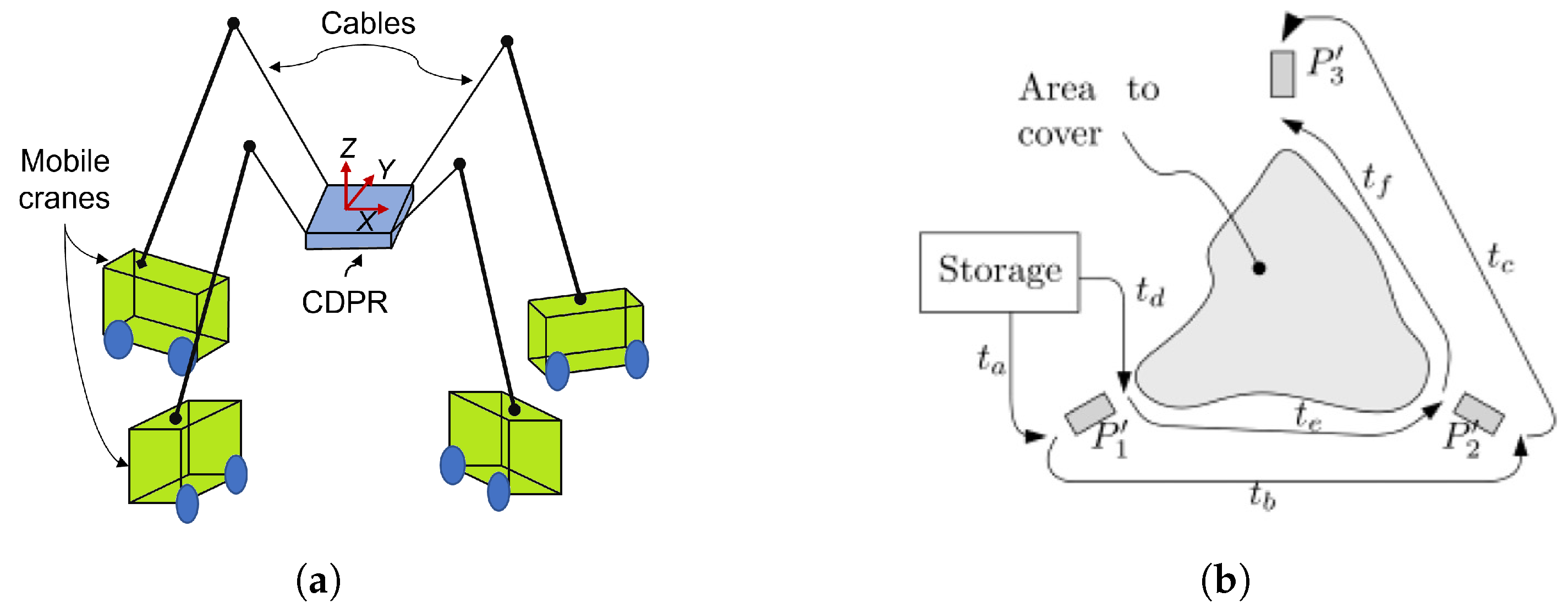
2.1. Mobile CDPRs
2.2. Multi-Objective Optimization
3. Methodology
3.1. Problem Statement
3.2. RUDE-AL Algorithm
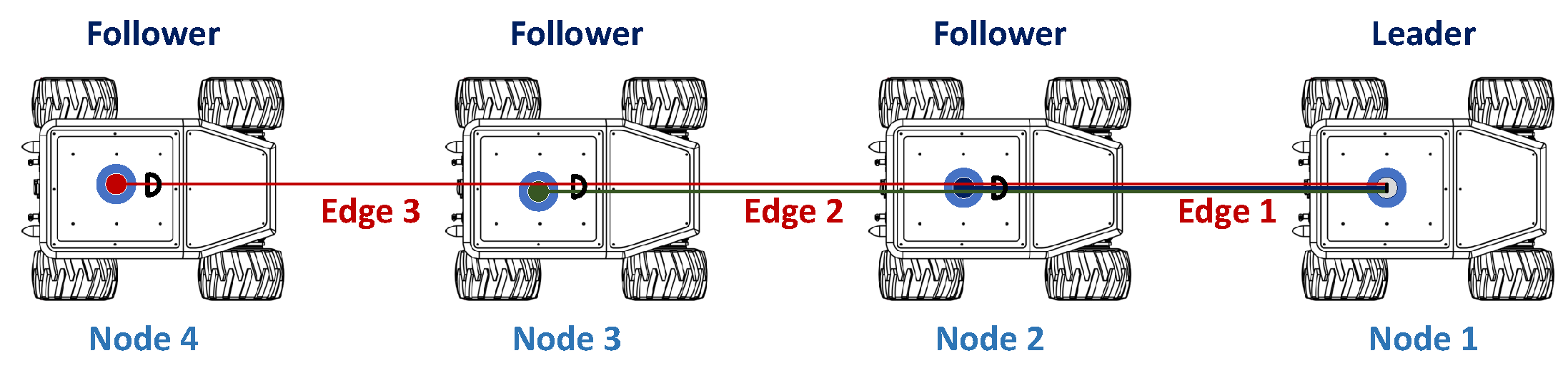
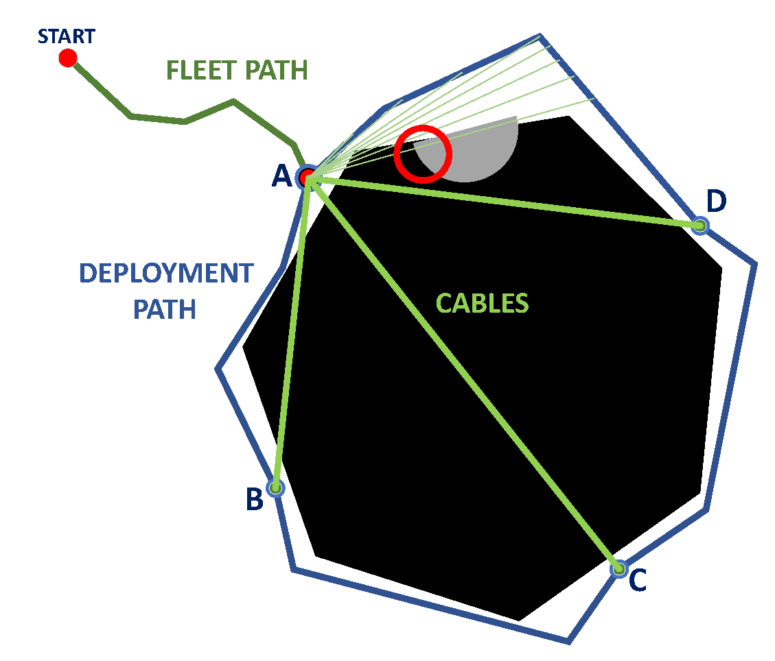
- Phase 1. Node-edge fleet configuration
- -
- Map, obstacle, and start selection for offline planning
- -
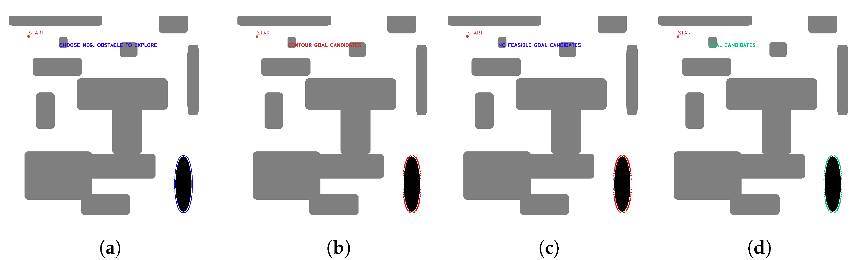
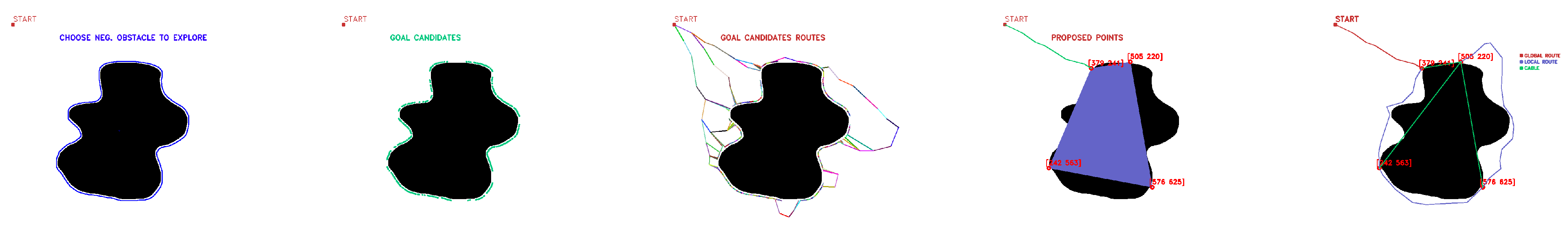
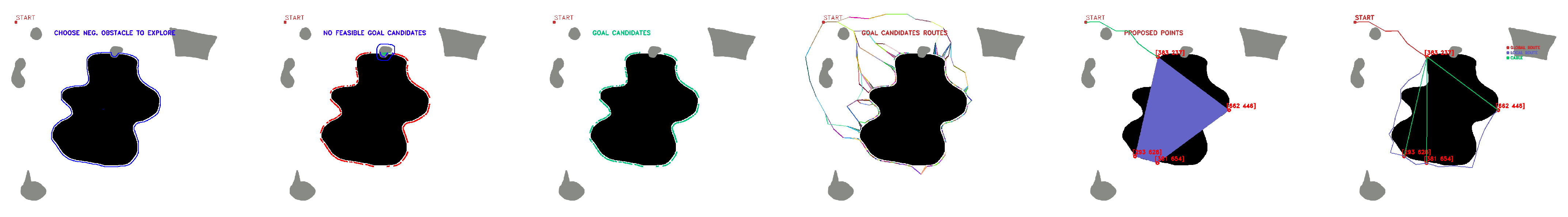
- Definition, sorting, and choosing of feasible goal candidates based on area coverage and distance cost of fleet deployment
- Phase 2. Roped individual configuration
- -
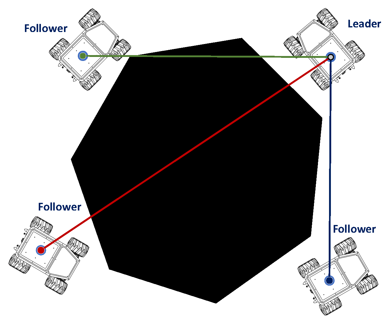
- Goal local planning and establishment of deployment configuration based on rope restrictions
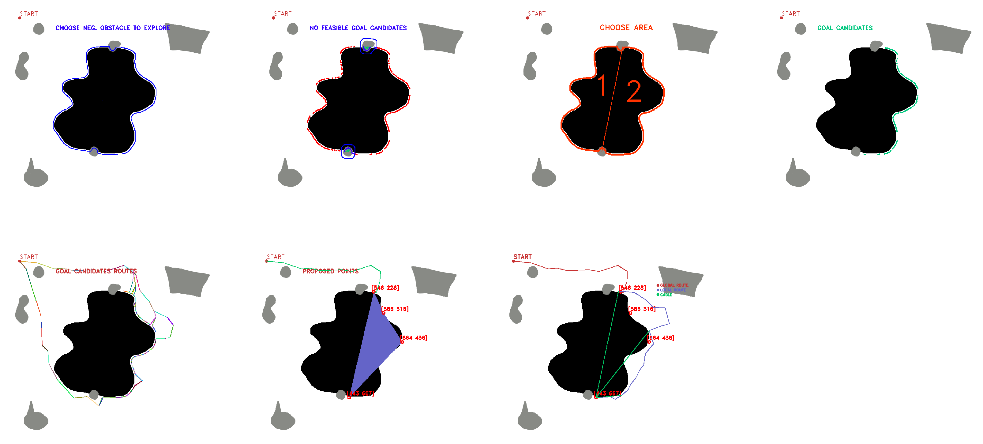
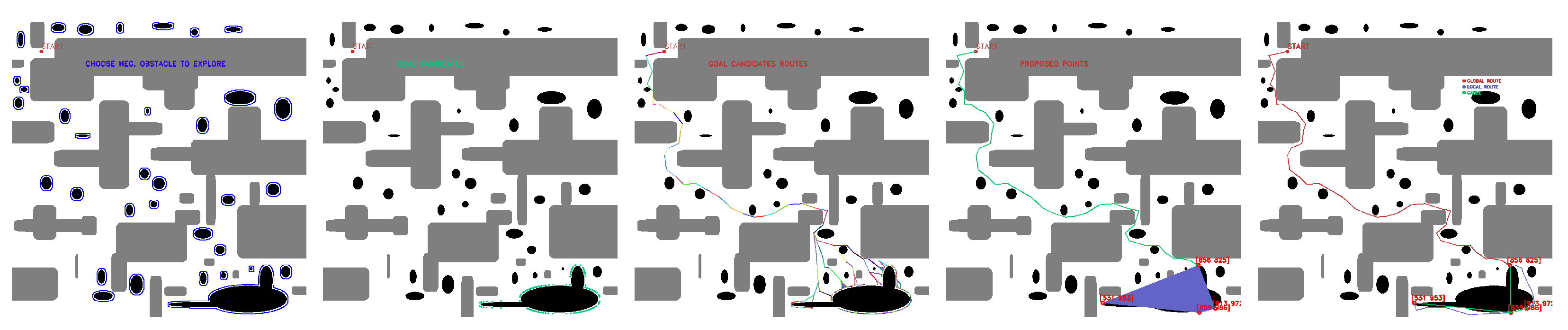
3.2.1. Phase 1. Node-Edge Fleet Configuration
Map, Obstacle, and Start Selection for Offline Planning
- Erode (line 12), Dilate (line 13), Range (line 14), Contours (line 16) and Centroids (line 18): are OpenCV functions used to inflate regions of images, define masks, and get characteristics of contours.
- Remove_dup (line 28): is a function to delete the multiple occurrences of an object in a list.
- Line(line 35): is a function that returns the slope and the constant “b” for a y = mx + b line between two input points
- Check_click (line 51): is a function that determines where the user clicks and returns the selected zone to explore (options are 1 or 2).
- Route (line 51) is a function that performs the prm path planning between two points. Returns the feasible path between them.
| Algorithm 1 Fleet Planning |
Input: map,start Output:
|
Definition, Sorting, and Choice of Feasible Goal Candidates Based on Area Coverage and Distance Cost of Fleet Deployment
- : covered area by points
- : vector between points 1–4
- : vector between points 1–3
- : vector between points 1–2
- : accumulated distance cost of route
- d: euclidean distance between points
- : fitness function
- : weight applied for area coverage
- : weight applied for path distance cost
- : covered by 4-candidate points combination
- : area of obstacle obtained from contours
- : vector of inverse normalized route cost for candidate points
- Get_area (line 13) is a function that gets the area of the contour made by a list of points. The output is the area of the contour.
- Route_cost (line 14) is a function that calculates the accumulated individual distance cost for a list of paths.
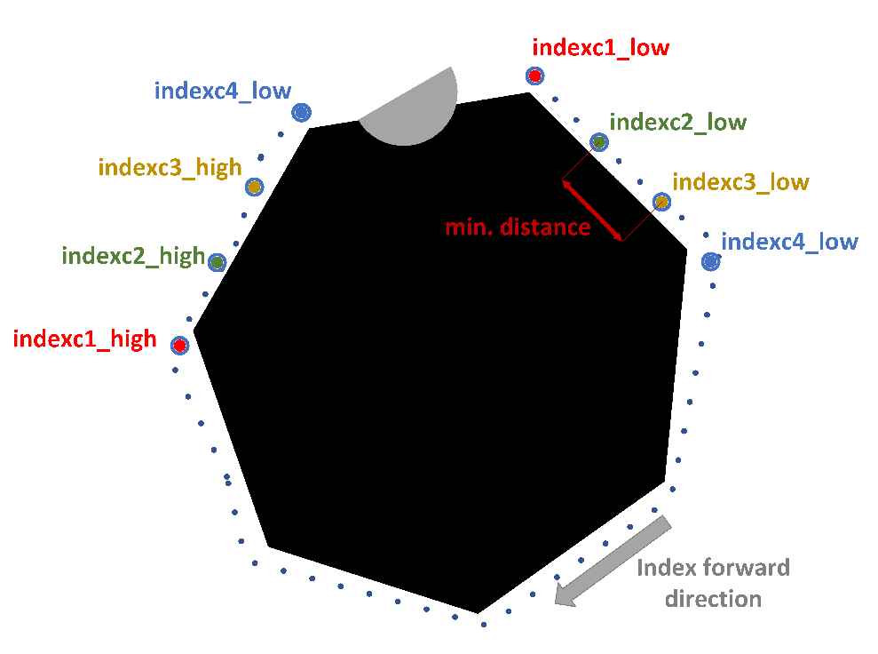
- Index_range (line 15) is a function that defines the lower and upper limit indexes for each candidate point according to a minimum distance between points. The output is a range of index for each of the four candidate points.
- Get_candidates (line 16) is a function that defines independent lists of candidate points of a main list according to the given limits. The output is four lists of points.
- Fitness_function (line 17) is a function that iterates testing different combinations according to Ga_instance parameters. It includes the Area_calc() in order to calculate area for every iteration different combination of points.
- Area_calc (line 17) is a function that calculates the area described between four points according to cross product and sum of areas described in Equation (1).
- Ga_instance (line 18) is pygad instance to configure the genetic algorithm that include the parameters described in Table 2. The instance must run using Ga_instance.run. The output of Ga_instance.best_solution() is the best combination of four points according to the fitness function.
| Algorithm 2 Points Selection |
Input: Output: sol_points,fleet_path
|
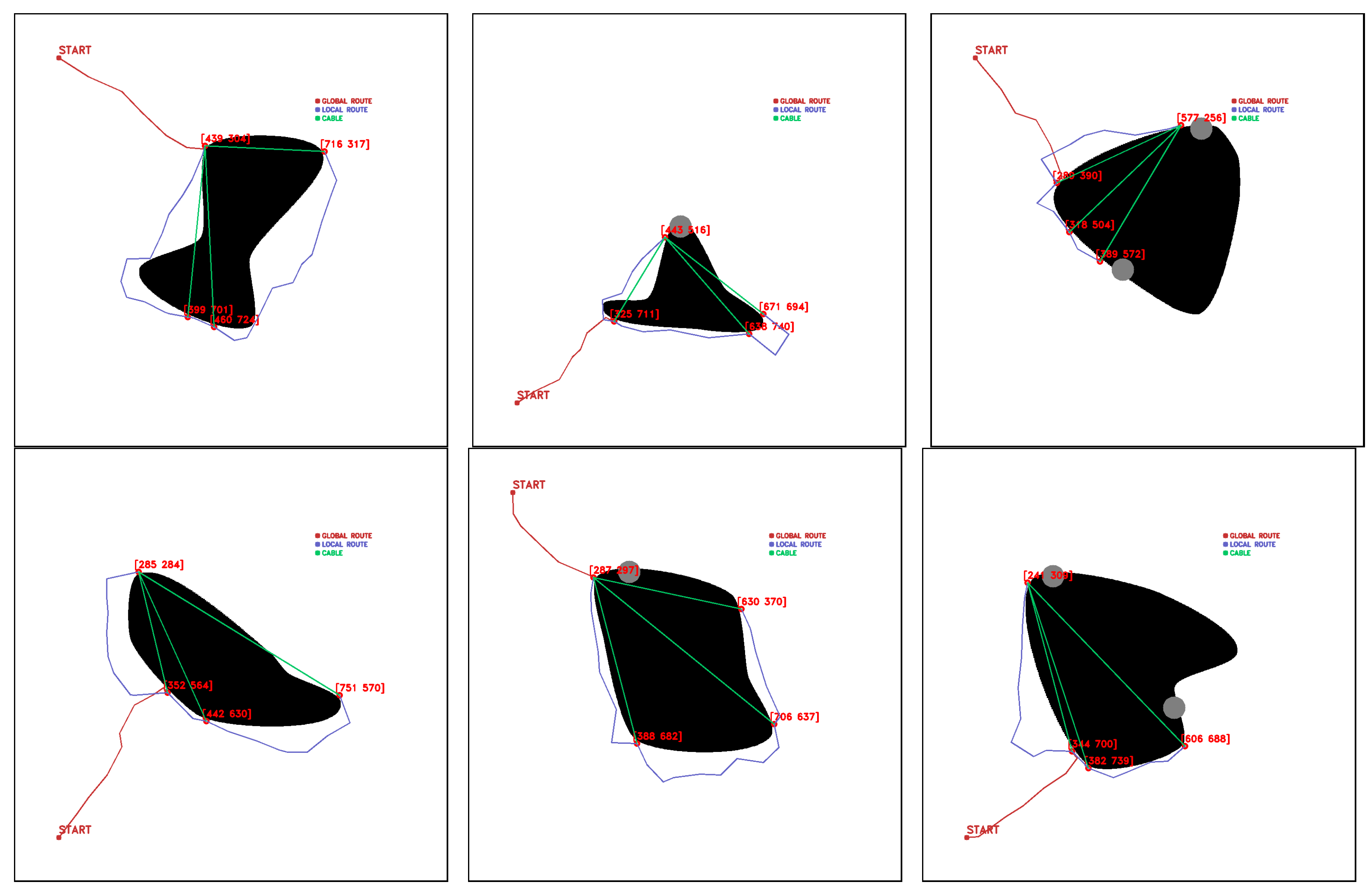
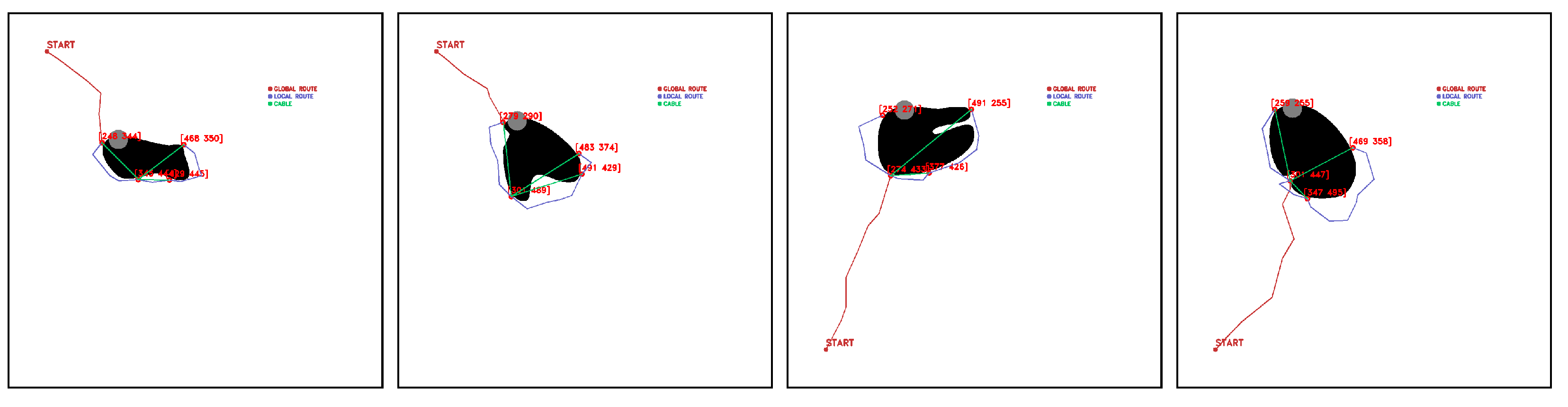
3.2.2. Phase 2. Roped Individual Configuration
Goal Local Planning and Establishment of Deployment Configuration Based on Rope Restrictions
- Route (line: 10) is a function that performs the PRM path planning between two points. It returns the feasible path between them.
- Route_check (line: 14) is a function that creates an interpolated line between input point and every interpolated point of the input route, and checks if there are collisions between the interpolated line (rope) and a positive obstacle. Output is a Boolean true if there is collision, and false if there is no collisions.
- GetRobotPaths (line: 35) is a function in which input is feasibility of each path of the roped configuration deployment check, and it returns the path for each robot according to Table 5.
| Algorithm 3 Roped deployment |
Input: Output:
|
4. Experiments
- Maps: The range of maps that are auto-generated with the indicated characteristics.
- : number of random points to connect to generate the Bezier curve.
- : radius around the points where control points are. A larger radius means a sharper feature.
- Smoothness: Parameter to define the smoothness of the curve.
- Scale: X and Y pixel rectangle size where the random points will be generated.
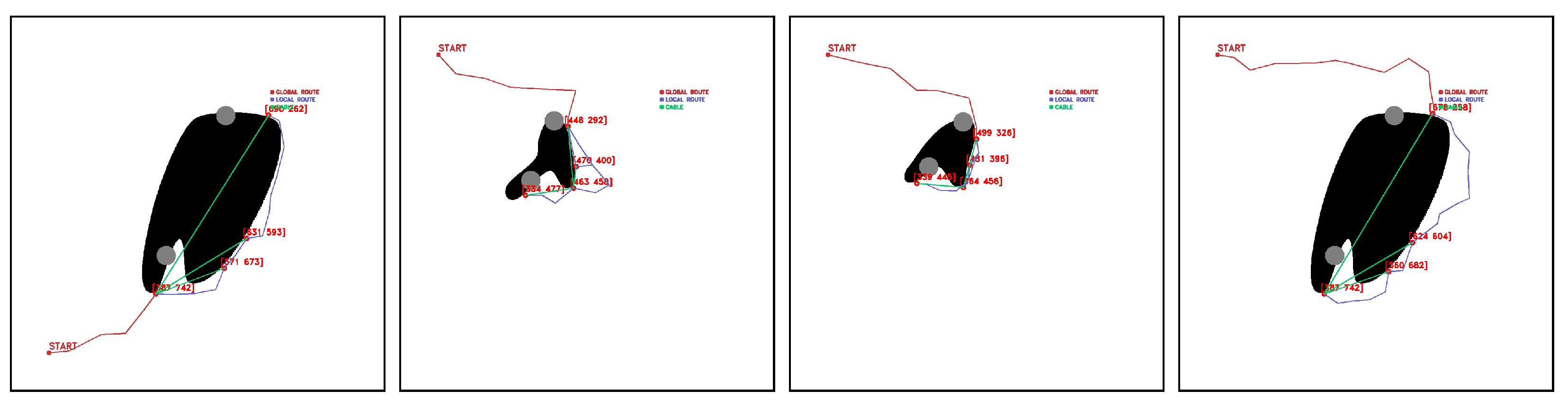
5. Results
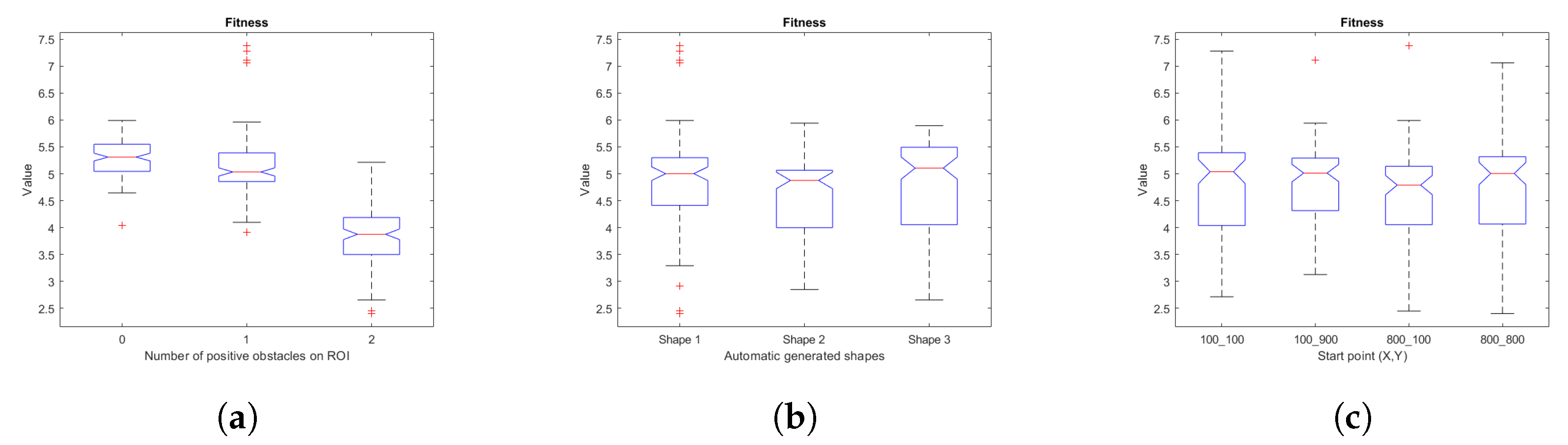
5.1. Fitness
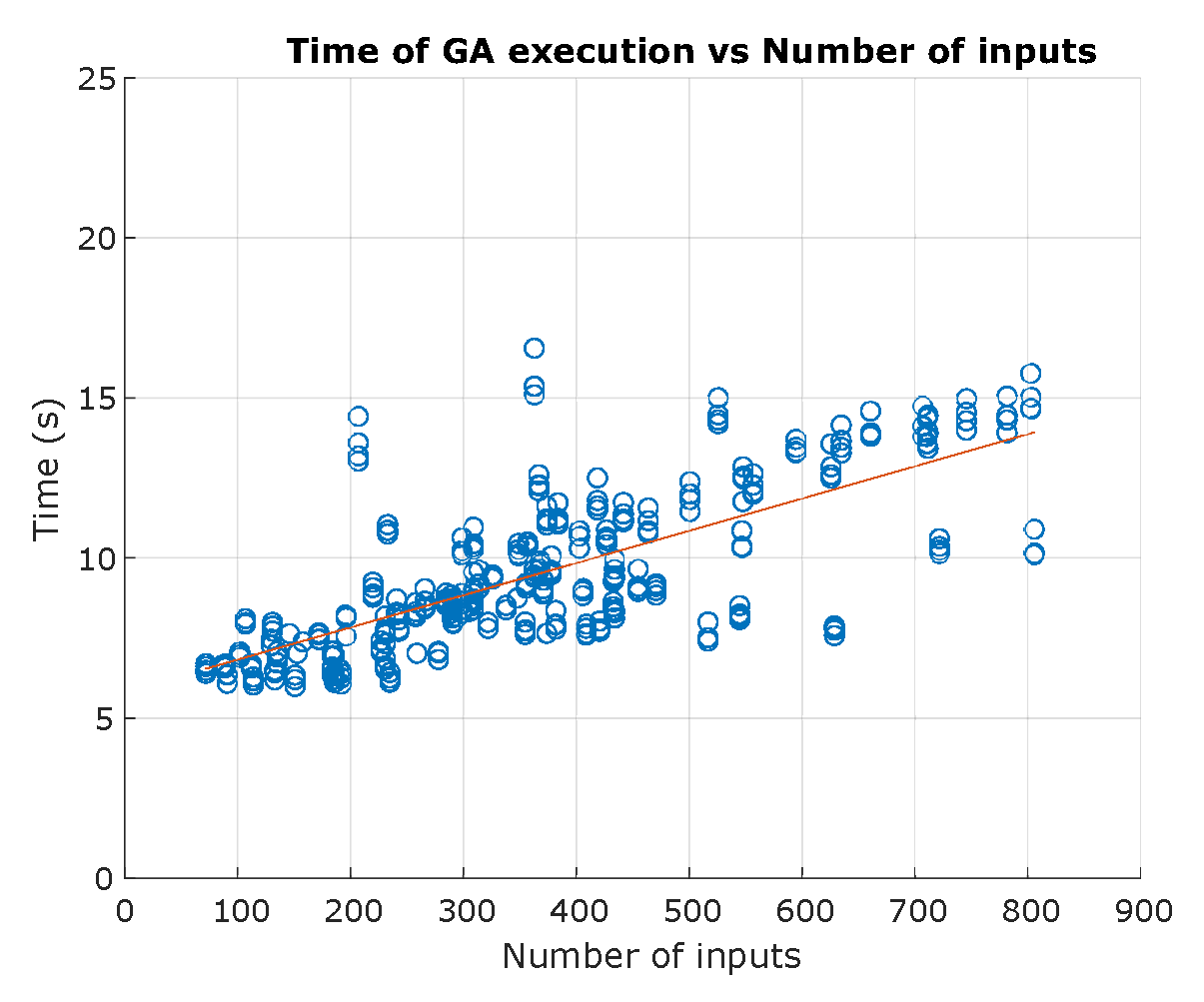
5.2. Algorithm Complexity
5.3. Test on Gazebo Simulator
6. Conclusions
Author Contributions
Funding
Institutional Review Board Statement
Informed Consent Statement
Data Availability Statement
Conflicts of Interest
Abbreviations
| ANOVA | Analysis of Variance |
| ASR | Air Sea Rescue |
| CDPR | Cable Driven Parallel Robot |
| CPRMC | Cable Parallel robot for multiple mobile cranes |
| DARPA | Defense Advanced Research Project Agency |
| EA | Evolutionary Algorithms |
| GA | Genetic Algorithms |
| MCDPR | Mobile Cable-Driven Parallel Robot |
| PRM | Probabilistic Roadmap |
| ROI | Region of Interest |
| RTS | Robotic Total Station |
| RUDE-AL | Roped UGV fleet Deployment ALgorithm |
| SAR | Search and Rescue |
| TS | Total Station |
| UGV | Unmanned Ground Vehicle |
| USAR | Urban Search and Rescue |
| WiSAR | Wilderness SAR |
Appendix A
Appendix B
References
- Maleki, M.; Salman, M.; Sahebi, S.; Szilard, V. GIS based sinkhole susceptibility mapping using the best worst method. Spat. Inf. Res. 2023. [Google Scholar] [CrossRef]
- La Rosa, A.; Pagli, C.; Molli, G.; Casu, F.; De Luca, C.; Pieroni, A.; D’Amato Avanzi, G. Growth of a sinkhole in a seismic zone of the northern Apennines (Italy). Nat. Hazards Earth Syst. Sci. 2018, 18, 2355–2366. [Google Scholar] [CrossRef]
- Montgomery, J.; Jackson, D.; Kiernan, M.; Anderson, J.B.; Ginn, S. Final Report for ALDOT Project 930-945 Use of Geophysical Methods for Sinkhole Exploration; Auburn University: Auburn, AL, USA, 2020; pp. 1–120. [Google Scholar]
- Liu, H.; Ge, J.; Wang, Y.; Li, J.; Ding, K.; Zhang, Z.; Guo, Z.; Li, W.; Lan, J. Multi-UAV Optimal Mission Assignment and Path Planning for Disaster Rescue Using Adaptive Genetic Algorithm and Improved Artificial Bee Colony Method. Actuators 2022, 11, 4. [Google Scholar] [CrossRef]
- Hermosilla, R.G. The Guatemala City sinkhole collapses. Carbonates Evaporites 2012, 27, 103–107. [Google Scholar] [CrossRef]
- English, S.; Heo, J.; Won, J. Investigation of sinkhole formation with human influence: A case study fromwink sink in Winkler county, Texas. Sustainability 2020, 12, 3537. [Google Scholar] [CrossRef]
- Ali, H.; Choi, J.H. A review of underground pipeline leakage and sinkhole monitoring methods based on wireless sensor networking. Sustainability 2019, 11, 4007. [Google Scholar] [CrossRef]
- Gutiérrez, F.; Benito-Calvo, A.; Carbonel, D.; Desir, G.; Sevil, J.; Guerrero, J.; Martínez-Fernández, A.; Karamplaglidis, T.; García-Arnay, Á.; Fabregat, I. Review on sinkhole monitoring and performance of remediation measures by high-precision leveling and terrestrial laser scanner in the salt karst of the Ebro Valley, Spain. Eng. Geol. 2019, 248, 283–308. [Google Scholar] [CrossRef]
- Munoz-Ceballos, N.D.; Suarez-Rivera, G. Performance criteria for evaluating mobile robot navigation algorithms: A review. Rev. Iberoam. Autom. Inform. Ind. 2022, 19, 132–143. [Google Scholar] [CrossRef]
- Kashino, Z.; Nejat, G.; Benhabib, B. Aerial Wilderness Search and Rescue with Ground Support. J. Intell. Robot. Syst. Theory Appl. 2020, 99, 147–163. [Google Scholar] [CrossRef]
- Reardon, C.; Fink, J. Air-ground robot team surveillance of complex 3D environments. In Proceedings of the SSRR 2016—International Symposium on Safety, Security and Rescue Robotics, Lausanne, Switzerland, 23–27 October 2016; pp. 320–327. [Google Scholar] [CrossRef]
- Delmerico, J.; Mueggler, E.; Nitsch, J.; Scaramuzza, D. Active autonomous aerial exploration for ground robot path planning. IEEE Robot. Autom. Lett. 2017, 2, 664–671. [Google Scholar] [CrossRef]
- Xiao, X.; Dufek, J.; Woodbury, T.; Murphy, R. UAV assisted USV visual navigation for marine mass casualty incident response. In Proceedings of the IEEE International Conference on Intelligent Robots and Systems, Vancouver, BC, Canada, 24–28 September 2017; pp. 6105–6110. [Google Scholar] [CrossRef]
- Adrian, R.; García, G.; Arias-Montiel, M. Prototipo Virtual de un Robot Móvil Multi-Terreno Para Aplicaciones de Búsqueda y Rescate Ballbot Lego NXT Control View Project Materiales de Construcción View Project; Technical Report October; Universidad Tecnologica de la Mixteca: Huajuapan de León, Mexico, 2016. [Google Scholar]
- Murphy, R.R.; Nardi, D.; Erkmen, A.M.; Fiorini, P. Search and Rescue Robotics. In Springer Handbook of Robotics; Springer: Berlin/Heidelberg, Germany, 2008. [Google Scholar] [CrossRef]
- Mehmood, S.; Ahmed, S.; Kristensen, A.S.; Ahsan, D. Multi criteria decision analysis (MCDA) of unmanned aerial vehicles (UAVS) as a part of standard response to emergencies. Int. J. Innov. Technol. Explor. Eng. 2018, 8, 79–85. [Google Scholar]
- Sung, Y. Multi-Robot Coordination for Hazardous Environmental Monitoring. Ph.D. Thesis, Virginia Polytechnic Institute and State University, Blacksburg, VA, USA, 2019. [Google Scholar]
- Merino, L.; Caballero, F.; Martínez-de Dios, J.R.; Ollero, A. Cooperative fire detection using unmanned aerial vehicles. Proc. IEEE Int. Conf. Robot. Autom. 2005, 2005, 1884–1889. [Google Scholar] [CrossRef]
- Brenner, S.; Gelfert, S.; Rust, H. New Approach in 3D Mapping and Localization for Search and Rescue Missions. In Proceedings of the CERC, Karlsruhe, Germany, 22–23 September 2017; pp. 105–111. [Google Scholar]
- Peña Queralta, J.; Taipalmaa, J.; Pullinen, B.C.; Katha Sarker, V.; Gia, T.N.; Tenhunen, H.; Gabbouj, M.; Raitoharju, J.; Westerlund, T. Collaborative Multi-Robot Systems for Search and Rescue: Coordination and Perception. 2020; pp. 1–28. Available online: http://xxx.lanl.gov/abs/2008.12610 (accessed on 29 May 2023).
- Fan, H.; Hernandez Bennetts, V.; Schaffernicht, E.; Lilienthal, A.J. Towards gas discrimination and mapping in emergency response scenarios using a mobile robot with an electronic nose. Sensors 2019, 19, 685. [Google Scholar] [CrossRef] [PubMed]
- Zhao, J.; Gao, J.; Zhao, F.; Liu, Y. A search-and-rescue robot system for remotely sensing the underground coal mine environment. Sensors 2017, 17, 2426. [Google Scholar] [CrossRef] [PubMed]
- Qian, S.; Zi, B.; Shang, W.W.; Xu, Q.S. A review on cable-driven parallel robots. Chin. J. Mech. Eng. (Engl. Ed.) 2018, 31, 66. [Google Scholar] [CrossRef]
- Surdilovic, D.; Radojicic, J.; Bremer, N. Efficient Calibration of Cable-Driven Parallel Robots with Variable Structure. Mech. Mach. Sci. 2015, 32, 113–128. [Google Scholar] [CrossRef]
- Bostelman, R.V.; Albus, J.S.; Dagalakis, N.G.; Jacoff, A. Robocrane project: An advanced concept for large scale manufacturing. In Proceedings of the Association for Unmanned Vehicles Systems International, Orlando, FL, USA, 1 July 1996. [Google Scholar]
- Pott, A.; Mütherich, H.; Kraus, W.; Schmidt, V.; Miermeister, P.; Verl, A. IPAnema: A family of cable-driven parallel robots for industrial applications. Mech. Mach. Sci. 2013, 12, 119–134. [Google Scholar] [CrossRef]
- El-ghazaly, G.; Gouttefarde, M.; Creuze, V. Adaptive Terminal Sliding Mode Control of a Manipulator: CoGiRo. In CableCon: Cable-Driven Parallel Robots; Springer: Cham, Switzerland, 2014; pp. 179–200. [Google Scholar]
- Miermeister, P.; Lächele, M.; Boss, R.; Masone, C.; Schenk, C.; Tesch, J.; Kerger, M.; Teufel, H.; Pott, A.; Bülthoff, H.H. The CableRobot simulator large scale motion platform based on Cable Robot technology. In Proceedings of the IEEE International Conference on Intelligent Robots and Systems, Daejeon, Republic of Korea, 9–14 October 2016; pp. 3024–3029. [Google Scholar] [CrossRef]
- Rodriguez-Barroso, A.; Saltaren, R. Cable-Driven Robot to Simulate the Buoyancy Force for Improving the Performance of Underwater Robots. In Cable-Driven Parallel Robots; Springer International Publishing: Cham, Switzerland, 2021; Volume 104, pp. 413–425. [Google Scholar] [CrossRef]
- Gouttefarde, M.; Lamaury, J.; Reichert, C.; Bruckmann, T. A Versatile Tension Distribution Algorithm for n-DOF Parallel Robots Driven by n + 2 Cables. IEEE Trans. Robot. 2015, 31, 1444–1457. [Google Scholar] [CrossRef]
- Pedemonte, N.; Rasheed, T.; Marquez-Gamez, D.; Long, P.; Hocquard, É.; Babin, F.; Fouché, C.; Caverot, G.; Girin, A.; Caro, S. FASTKIT: A Mobile Cable-Driven Parallel Robot for Logistics. Springer Tracts Adv. Robot. 2020, 132, 141–163. [Google Scholar] [CrossRef]
- Merlet, J.P. MARIONET, a family of modular wire-driven parallel robots. In Advances in Robot Kinematics: Motion in Man and Machine; Springer: Dordrecht, The Netherlands, 2010. [Google Scholar] [CrossRef]
- Rasheed, T. Collaborative Mobile Cable-Driven Parallel Robots. Ph.D. Thesis, L’ÉCole Centrale De Nantes, Nantes, France, 2020. [Google Scholar]
- Zi, B.; Lin, J.; Qian, S. Localization, obstacle avoidance planning and control of a cooperative cable parallel robot for multiple mobile cranes. Robot. Comput.-Integr. Manuf. 2015, 34, 105–123. [Google Scholar] [CrossRef]
- Tan, H.; Nurahmi, L.; Pramujati, B.; Caro, S. On the Reconfiguration of Cable-Driven Parallel Robots with Multiple Mobile Cranes. In Proceedings of the 2020 5th International Conference on Robotics and Automation Engineering (ICRAE), Singapore, 20–22 November 2020; Volume 1, pp. 126–130. [Google Scholar] [CrossRef]
- Seriani, S.; Gallina, P.; Wedler, A. A modular cable robot for inspection and light manipulation on celestial bodies. Acta Astronaut. 2016, 123, 145–153. [Google Scholar] [CrossRef]
- Aguilar, W.G.; Morales, S.; Ruiz, H.; Abad, V. RRT* GL Based Optimal Path Planning for Real-Time Navigation of UAVs. In Lecture Notes in Computer Science; Springer: Cham, Switzerland, 2017; pp. 585–595. [Google Scholar] [CrossRef]
- Zhu, Z.; Xiao, J.; Li, J.Q.; Wang, F.; Zhang, Q. Global path planning of wheeled robots using multi-objective memetic algorithms. Integr. Comput.-Aided Eng. 2015, 22, 387–404. [Google Scholar] [CrossRef]
- Cui, Y.; Geng, Z.; Zhu, Q.; Han, Y. Review: Multi-objective optimization methods and application in energy saving. Energy 2017, 125, 681–704. [Google Scholar] [CrossRef]
- Yu, W.; Li, B.; Jia, H.; Zhang, M.; Wang, D. Application of multi-objective genetic algorithm to optimize energy efficiency and thermal comfort in building design. Energy Build. 2015, 88, 135–143. [Google Scholar] [CrossRef]
- Feng, Z.; Niu, W.; Cheng, C. Optimization of hydropower reservoirs operation balancing generation benefit and ecological requirement with parallel multi-objective genetic algorithm. Energy 2018, 153, 706–718. [Google Scholar] [CrossRef]
- Ramli, M.A.; Bouchekara, H.R.; Alghamdi, A.S. Optimal sizing of PV/wind/diesel hybrid microgrid system using multi-objective self-adaptive differential evolution algorithm. Renew. Energy 2018, 121, 400–411. [Google Scholar] [CrossRef]
- Hormozi, M.A.; Zaki Dizaji, H.; Bahrami, H.; Sharifyazdi, M.; Monjezi, N. Multi-objective optimization of allocating sustainable mechanization for spraying and harvesting systems in paddy fields. Iran. J. Biosyst. Eng. 2023. [Google Scholar] [CrossRef]
- Xue, Y. Mobile Robot Path planning with a non-dominated sorting genetic algorithm. Appl. Sci. 2018, 8, 2253. [Google Scholar] [CrossRef]
- Xue, Y.; Sun, J.Q. Solving the path planning problem in mobile robotics with the multi-objective evolutionary algorithm. Appl. Sci. 2018, 8, 1425. [Google Scholar] [CrossRef]
- Pham, V.T.; Stefek, A.; Krivanek, V.; Nguyen, T.S. Design of a Saving-Energy Fuzzy Logic Controller for a Differential Drive Robot Based on an Optimization. Appl. Sci. 2023, 13, 997. [Google Scholar] [CrossRef]
- Kouritem, S.A.; Abouheaf, M.I.; Nahas, N.; Hassan, M. A multi-objective optimization design of industrial robot arms. Alex. Eng. J. 2022, 61, 12847–12867. [Google Scholar] [CrossRef]
- Yin, L.; Liu, J.; Zhou, F.; Gao, M.; Li, M. Cost-based hierarchy genetic algorithm for service scheduling in robot cloud platform. J. Cloud Comput. 2023, 12, 35. [Google Scholar] [CrossRef]
- Le, A.V.; Parween, R.; Mohan, R.E.; Nhan, N.H.K.; Abdulkader, R.E. Optimization complete area coverage by reconfigurable htrihex tiling robot. Sensors 2020, 20, 3170. [Google Scholar] [CrossRef] [PubMed]
- Kulich, M.; Kubalík, J.; Přeučil, L. An integrated approach to goal selection in mobile robot exploration. Sensors 2019, 19, 1400. [Google Scholar] [CrossRef]
- Rasheed, T.; Long, P.; Roos, A.S.; Caro, S. Optimization based Trajectory Planning of Mobile Cable-Driven Parallel Robots. In Proceedings of the IEEE International Conference on Intelligent Robots and Systems, Macau, China, 3–8 November 2019; pp. 6788–6793. [Google Scholar] [CrossRef]
- Gad, A.F. PyGAD: An Intuitive Genetic Algorithm Python Library. 2021. Available online: http://xxx.lanl.gov/abs/2106.06158 (accessed on 29 May 2023).
- Vailland, G.; Gouranton, V.; Babel, M. Cubic Bézier Local Path Planner for Non-holonomic Feasible and Comfortable Path Generation. In Proceedings of the IEEE International Conference on Robotics and Automation, Xi’an, China, 30 May–5 June 2021; pp. 7894–7900. [Google Scholar] [CrossRef]
- Bermúdez Salguero, D.J. Métodos de Ayuda a la Navegación en Exteriores Para Robot Summit en Entorno ROS. Ph.D. Thesis, Universidad de Sevilla Escuela Técnica Superior de Ingeniería, Sevilla, Spain, 2022. [Google Scholar]
- Abdiansah, A.; Wardoyo, R. Time Complexity Analysis of Support Vector Machines (SVM) in LibSVM. Int. J. Comput. Appl. 2015, 128, 28–34. [Google Scholar] [CrossRef]


| Reference | Robot Name | Mobile Bases | Application | Environment | Physical Implementation | Number of Robotic Platforms | Degrees of Freedom |
|---|---|---|---|---|---|---|---|
| [25] | Robocrane | YES | Research | Indoor/Outdoor | YES | 3 | 6 |
| [26] | IPAnema | NO | Industry | Indoor | YES | 1 | 6 |
| [27] | CoGiro | NO | Research | Indoor | YES | 1 | 6 |
| [28] | CableRobot | NO | Research | Indoor | YES | 1 | 6 |
| [29] | - | NO | Research | Indoor | YES | 1 | 6 |
| [30] | CABLAR | NO | Logistics | Indoor | YES | 1 | 6 |
| [31] | FASTKIT | YES | Logistics | Indoor | YES | 2 | 6 |
| [32] | MARIONET-CRANE | YES | Rescue | Outdoor | YES | 1 | 6 |
| [33] | MoPick | YES | Logistics | Indoor | YES | 4 | 3 |
| [34] | - | YES | Research | Outdoor | NO | 4 | 4 |
| [35] | - | YES | Research | Outdoor | NO | 3 | 3 |
| [36] | - | YES | Research | Outdoor | NO | 3 | 3 |
| Tipo | RGB Color | UGVs Navigation Allowed | Cable Cross Allowed |
|---|---|---|---|
| Free space | (255, 255, 255) | YES | YES |
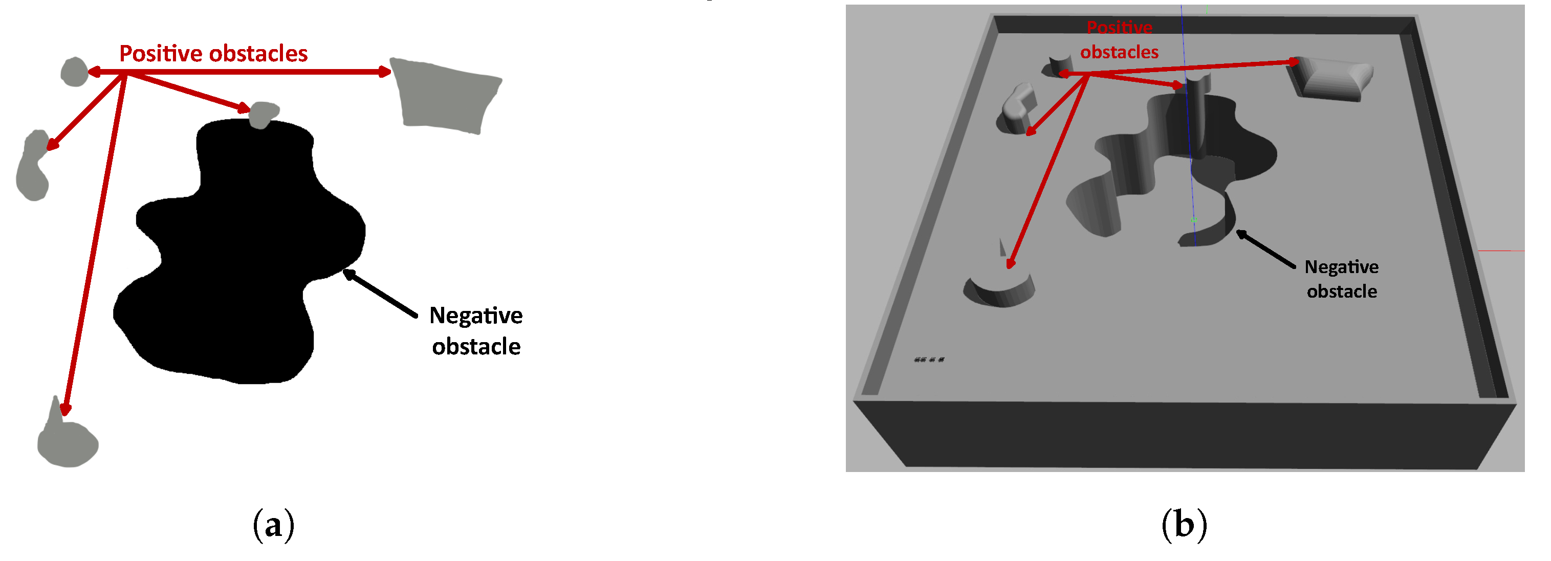
| Positive obstacle | (136, 138, 133) | NO | NO |
| Negative obstacle | (0, 0, 0) | NO | YES |
| Parameter | Definition | Value |
|---|---|---|
| num_generations | Number of generations | 1200 |
| mutation_num_genes | Number of genes por instance random_mutation() | 4 |
| num_parents_mating | Number of solutions to be selected as parents | 2 |
| sol_per_pop | Number of solutions in the population | 70 |
| num_genes | Number of genes in each solution | 4 |
| fitness_function | Fitness function | |
| init_range_low | Lower value of random range where initial population is selected. | 0 |
| init_range_high | Upper value of random range where initial population is selected. | len(candidate1)/2 |
| crossover_type | Type of crossover operation. | “single_point” |
| random_mutation_min_val | Start value of the range from which a random value is selected to be added to the gene. | 1 |
| random_mutation_max_val | End value of the range from which a random value is selected to be added to the gene. | 100 |
| mutation_type | Type of mutation operation | “random” |
| gene_space | Specify the posible values for each gene in order to restrict the gene values. | [range (0, len(candidate1)), range (0, len(candidate2)), range (0, len(candidate3)), range (0, len(candidate4)) ] |
| gene_type | Gene type (numeric data type) | int |
| Point | 1st Feasible Path | 2nd Feasible Path | 3rd Feasible Path | Feasible Configuration |
|---|---|---|---|---|
| A | A →(,,) | |||
| A →(,,) | ||||
| A →(,,) | ||||
| A →(,,) | ||||
| B | B →(,,) | |||
| B →(,,) | ||||
| B →(,,) | ||||
| B →(,,) | ||||
| C | C →(,,) | |||
| C →(,,) | ||||
| C →(,,) | ||||
| C →(,,) | ||||
| D | D →(,,) | |||
| D →(,,) | ||||
| D →(,,) | ||||
| D →(,,) |
| Principal Node Point | Feasible Configuration | Robot 1 Path | Robot 2 Path | Robot 3 Path | Robot 4 Path |
|---|---|---|---|---|---|
| A | type 1 | FP+ADCB | FP + ADC | FP + AD | FP |
| type 2 | FP + ABCD | FP + ABC | FP + AB | FP | |
| type 3 | FP + ADC | FP + AD | FP + AB | FP | |
| type 4 | FP + ABC | FP + AB | FP + AD | FP | |
| B | type 1 | FP + BADC | FP + BAD | FP + BA | FP |
| type 2 | FP + BCDA | FP + BCD | FP + BC | FP | |
| type 3 | FP + BAD | FP + BA | FP + BC | FP | |
| type 4 | FP + BCD | FP + BC | FP + BA | FP | |
| C | type 1 | FP + CBAD | FP + CBA | FP + CB | FP |
| type 2 | FP + CDAB | FP + CDA | FP + CD | FP | |
| type 3 | FP + CBA | FP + CB | FP + CD | FP | |
| type 4 | FP + CDA | FP + CD | FP + CB | FP | |
| D | type 1 | FP + DCBA | FP + DCB | FP + DC | FP |
| type 2 | FP + DABC | FP + DAB | FP + DA | FP | |
| type 3 | FP + DCB | FP + DC | FP + DA | FP | |
| type 4 | FP + DAB | FP + DA | FP + DC | FP |
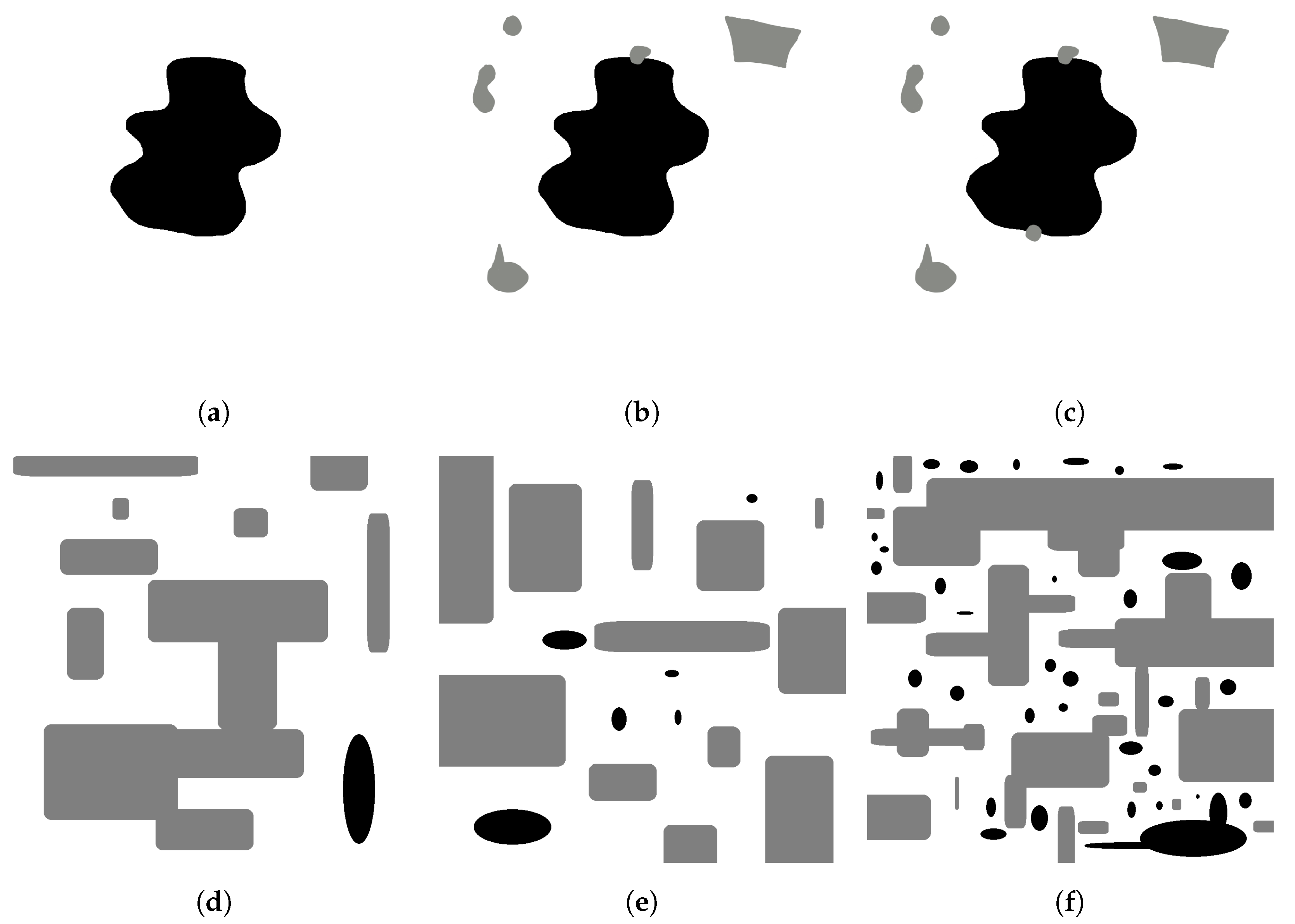
| Map | Number of Positive Obstacles | Number of Negative Obstacles | Number of Positive Obstacles around ROI | Shape of Negative Obstacle |
|---|---|---|---|---|
| 1 | 0 | 1 | 0 | Irregular |
| 2 | 4 | 1 | 1 | Irregular |
| 3 | 5 | 1 | 2 | Irregular |
| 4 | 8 | 1 | 0 | Ellipse |
| 5 | 12 | 6 | 0 | Ellipse |
| 6 | 17 | 34 | 0 | Irregular ellipse |
| Maps | Number of Positive Obstacles around ROI | Smoothness | Scale | ||
|---|---|---|---|---|---|
| 1–10 | 0–2 | 0.2 | 0.05 | 6 | 500 |
| 11–20 | 0–2 | 0.3 | 0.08 | 7 | 250 |
| 21–30 | 0–2 | 0.1 | 0.1 | 8 | 300 |
| Experiment | Number of Maps | Number of Experiments | Number of Successful Experiments | Successful Rate |
|---|---|---|---|---|
| Global TEST | 6 | 24 | 24 | 100% |
| SHAPE TEST (feasible paths) | 90 | 360 | 357 | 99.16% |
| SHAPE TEST (feasible paths with workspace limitation) | 90 | 360 | 352 | 97.78% |
| SHAPE TEST (feasible paths with collision risk) | 90 | 360 | 350 | 97.2% |
| SHAPE TEST (feasible paths with exceptions) | 90 | 360 | 354 | 98.33% |
| SHAPE TEST | 90 | 360 | 333 | 92.5% |
Disclaimer/Publisher’s Note: The statements, opinions and data contained in all publications are solely those of the individual author(s) and contributor(s) and not of MDPI and/or the editor(s). MDPI and/or the editor(s) disclaim responsibility for any injury to people or property resulting from any ideas, methods, instructions or products referred to in the content. |
© 2023 by the authors. Licensee MDPI, Basel, Switzerland. This article is an open access article distributed under the terms and conditions of the Creative Commons Attribution (CC BY) license (https://creativecommons.org/licenses/by/4.0/).
Share and Cite
Orbea, D.; Cruz Ulloa, C.; Del Cerro, J.; Barrientos, A. RUDE-AL: Roped UGV Deployment Algorithm of an MCDPR for Sinkhole Exploration. Sensors 2023, 23, 6487. https://doi.org/10.3390/s23146487
Orbea D, Cruz Ulloa C, Del Cerro J, Barrientos A. RUDE-AL: Roped UGV Deployment Algorithm of an MCDPR for Sinkhole Exploration. Sensors. 2023; 23(14):6487. https://doi.org/10.3390/s23146487
Chicago/Turabian StyleOrbea, David, Christyan Cruz Ulloa, Jaime Del Cerro, and Antonio Barrientos. 2023. "RUDE-AL: Roped UGV Deployment Algorithm of an MCDPR for Sinkhole Exploration" Sensors 23, no. 14: 6487. https://doi.org/10.3390/s23146487
APA StyleOrbea, D., Cruz Ulloa, C., Del Cerro, J., & Barrientos, A. (2023). RUDE-AL: Roped UGV Deployment Algorithm of an MCDPR for Sinkhole Exploration. Sensors, 23(14), 6487. https://doi.org/10.3390/s23146487