
An Affordable Streamflow Measurement Technique Based on Delay and Sum Beamforming

 ,
,  ,
,  ,
,  , , , ,
Abstract
:1. Introduction
2. Materials and Methods
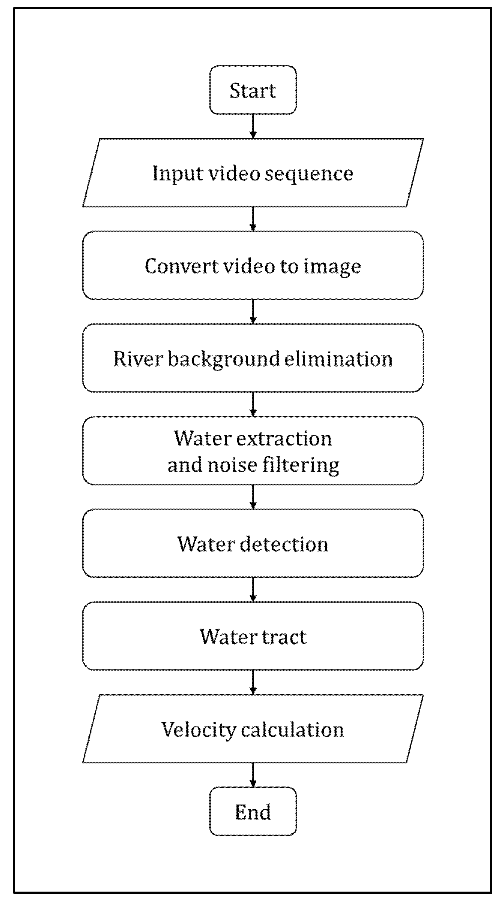
2.1. Beamforming Imaging Based Algorithms
2.1.1. MUSIC
Estimating the Exact Number of Targets
Minimum Description Length
Eigenvalue Gradients
Detecting Moving Targets and Measuring Velocity
2.1.2. Doppler Processing
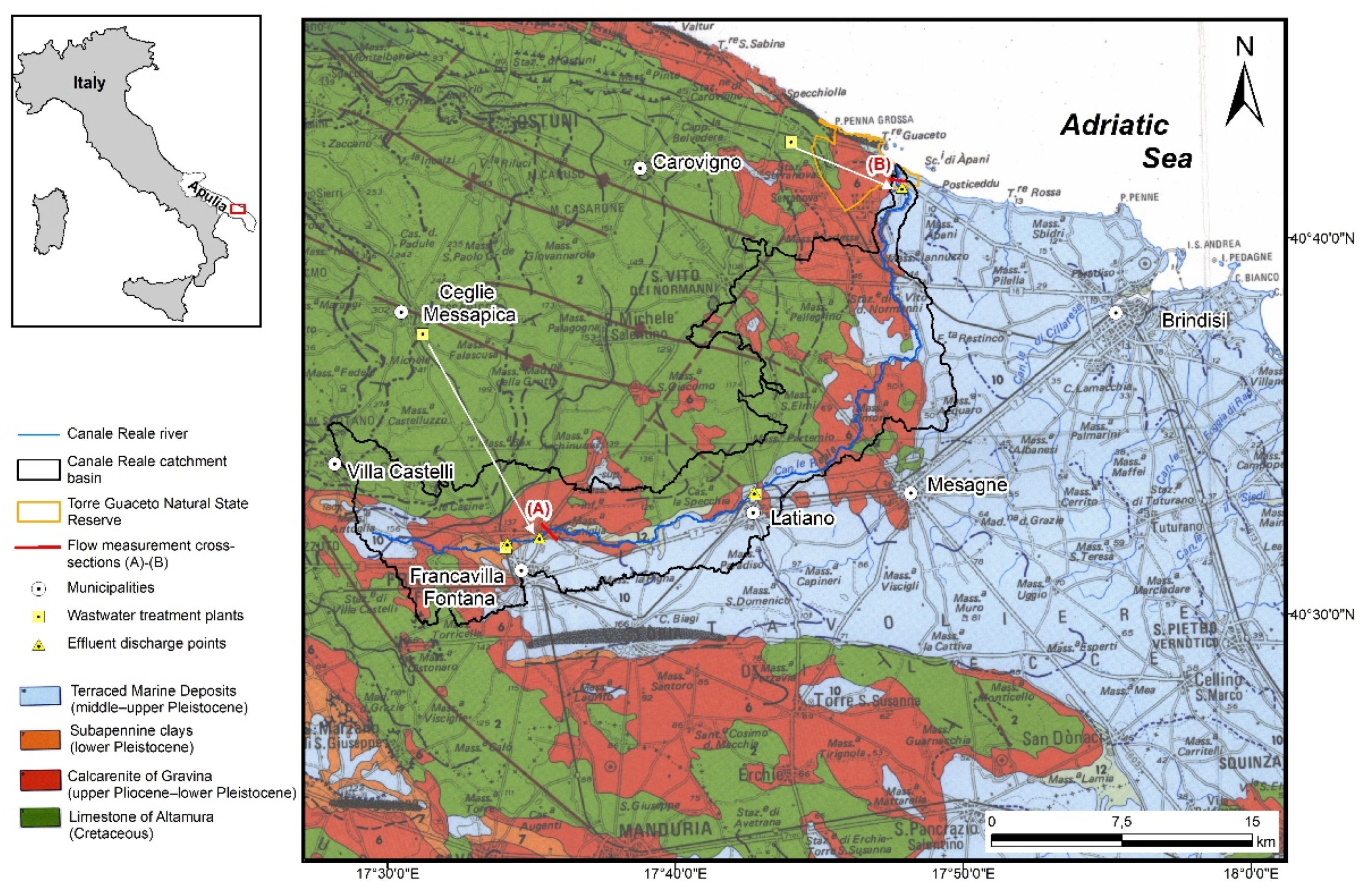
3. Study Area
3.1. Groundwater
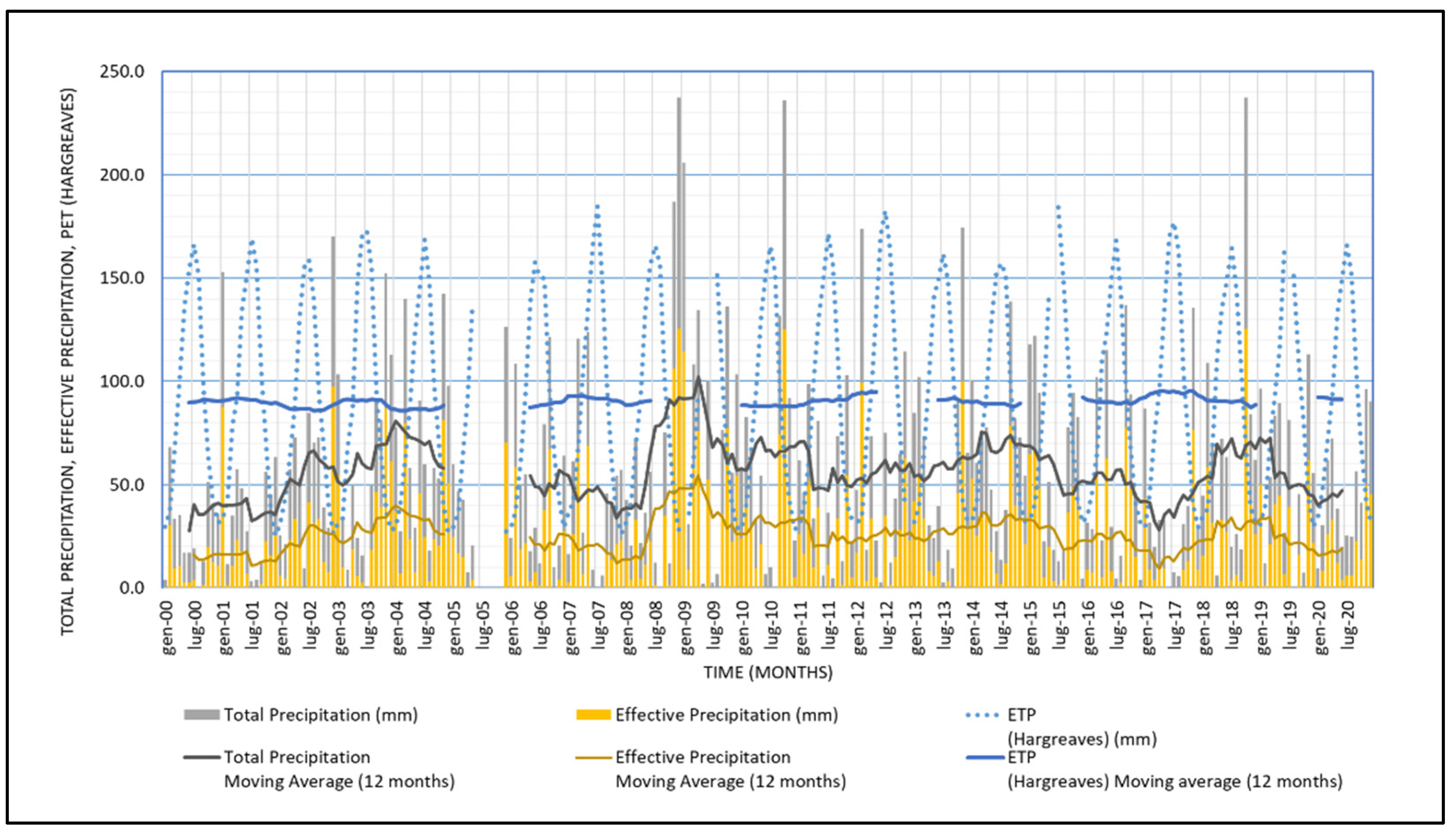
3.2. Climate
3.3. Main Environmental Issues
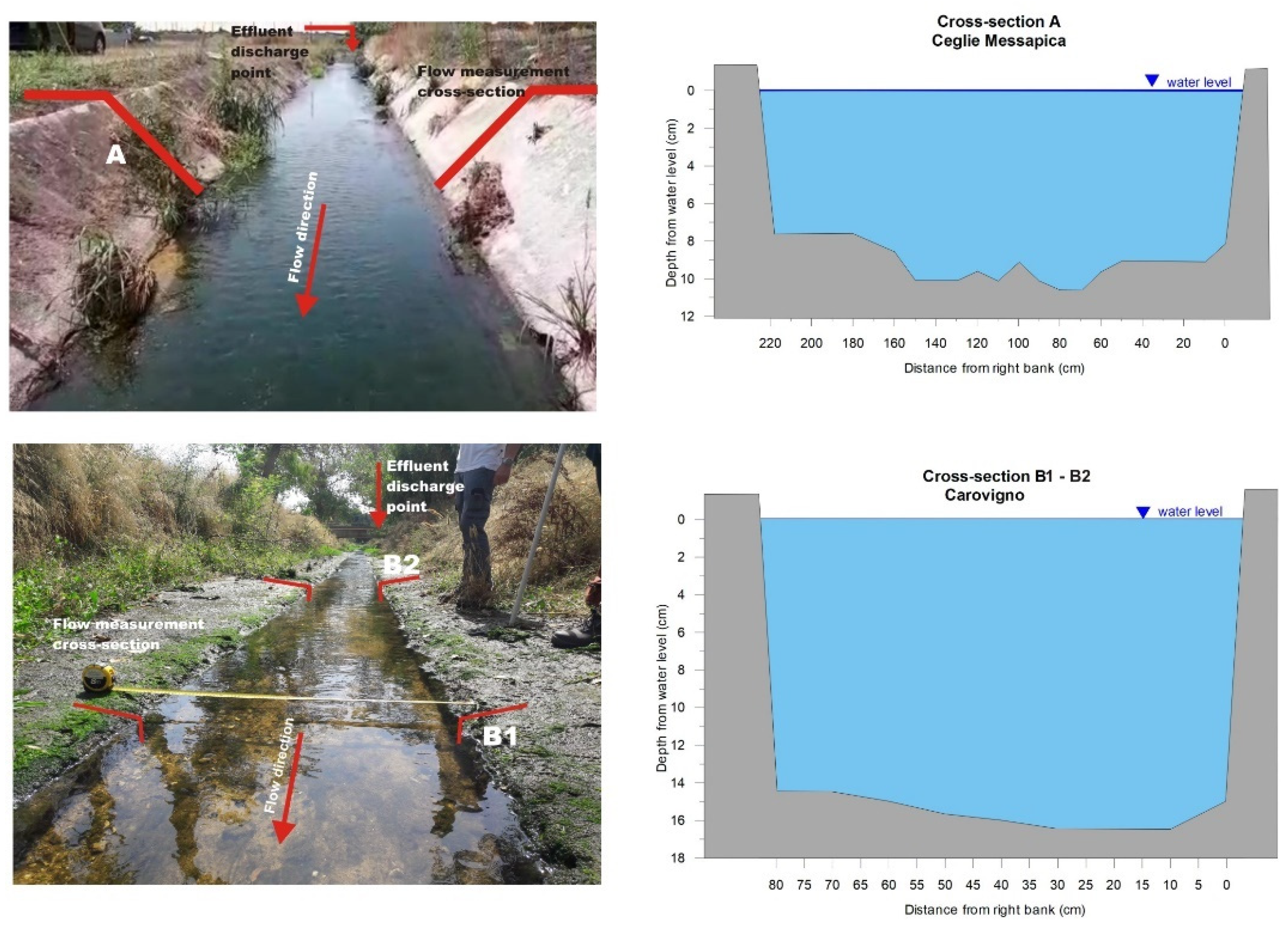
3.4. In Field Measurement and Video
4. Results and Discussion
4.1. Methodology Outcomes
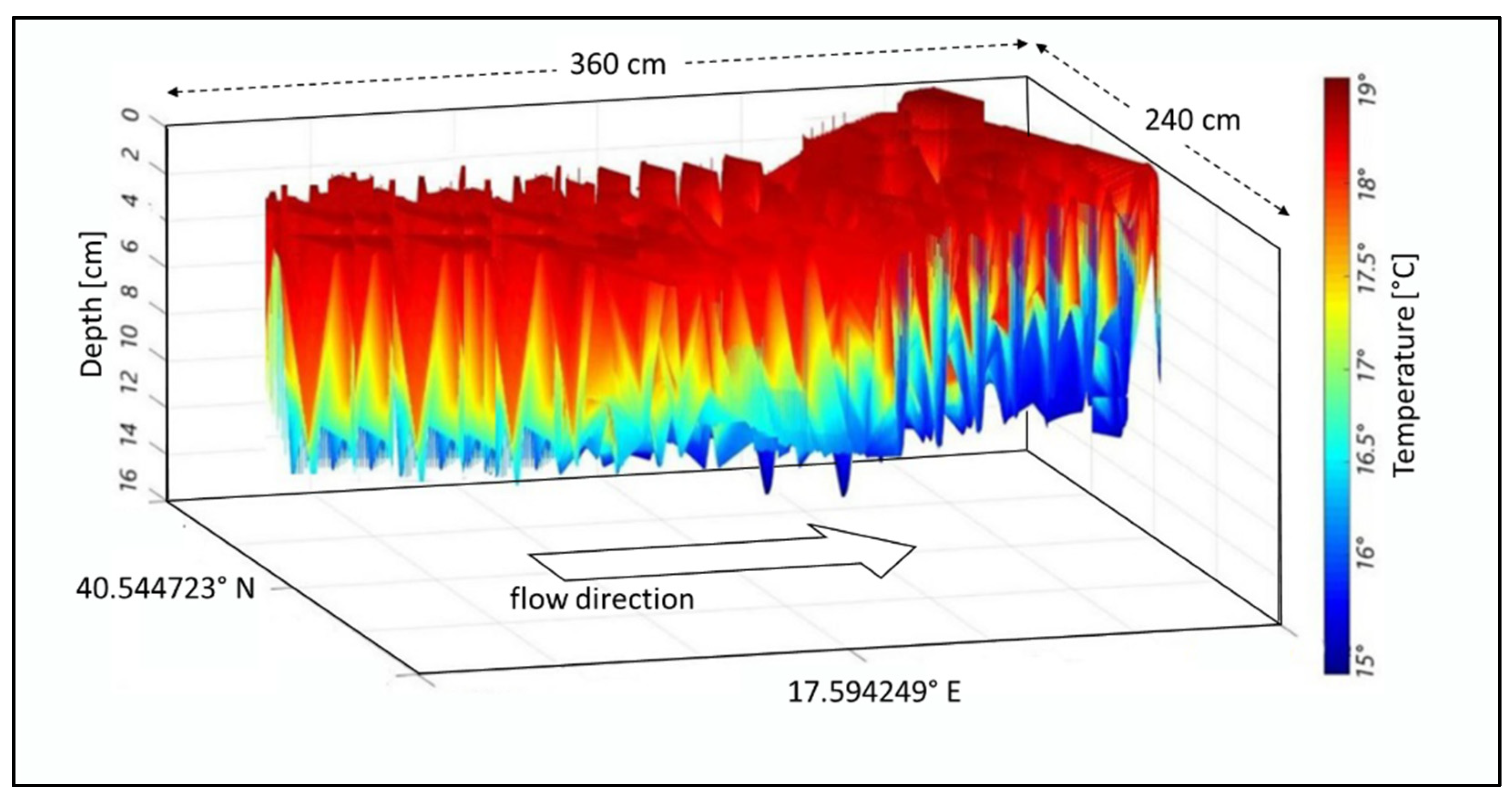
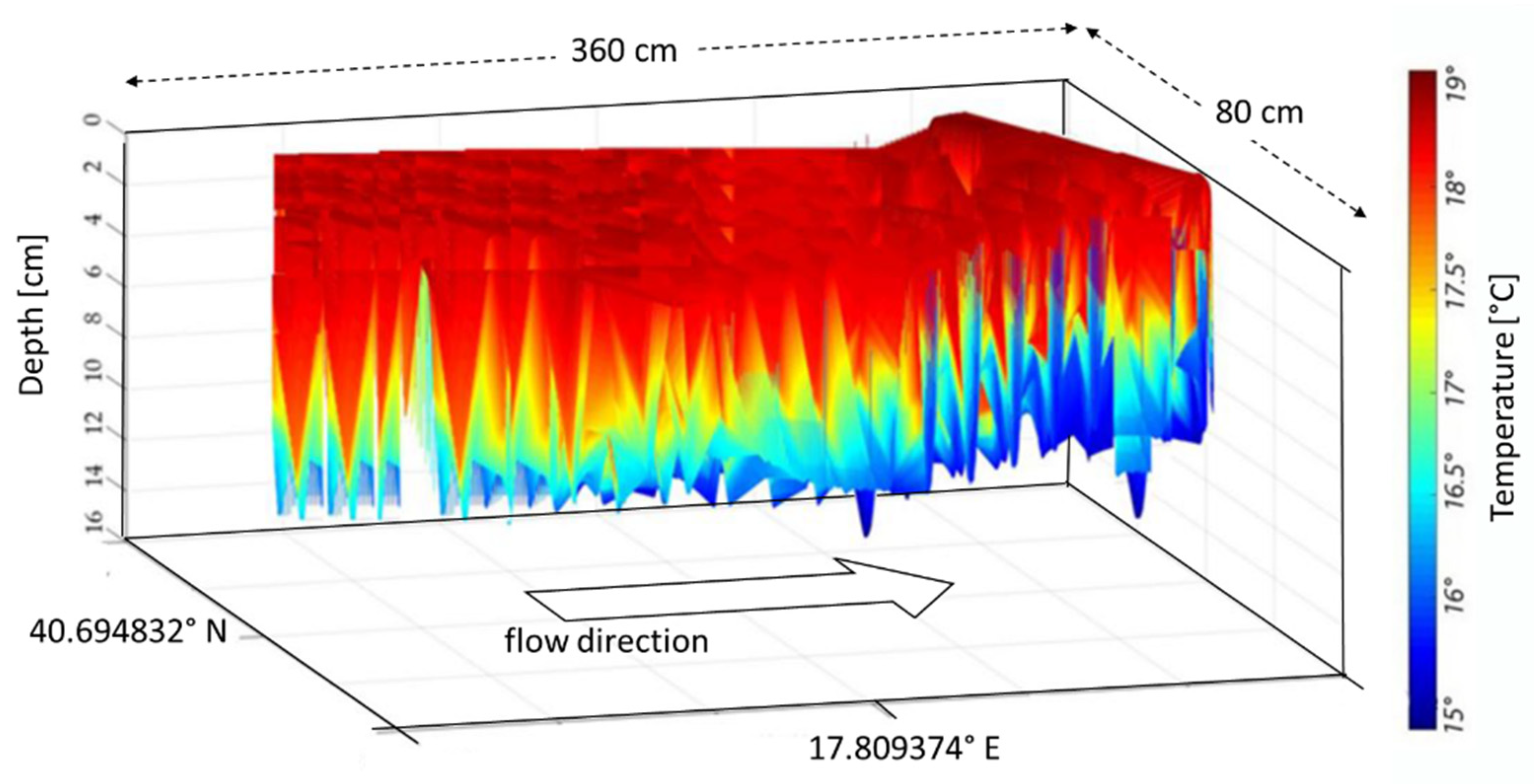
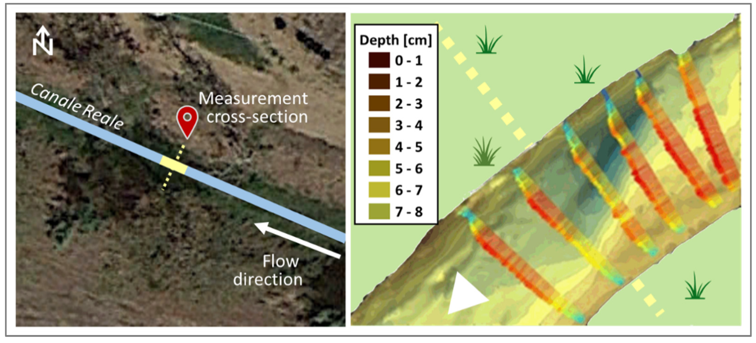
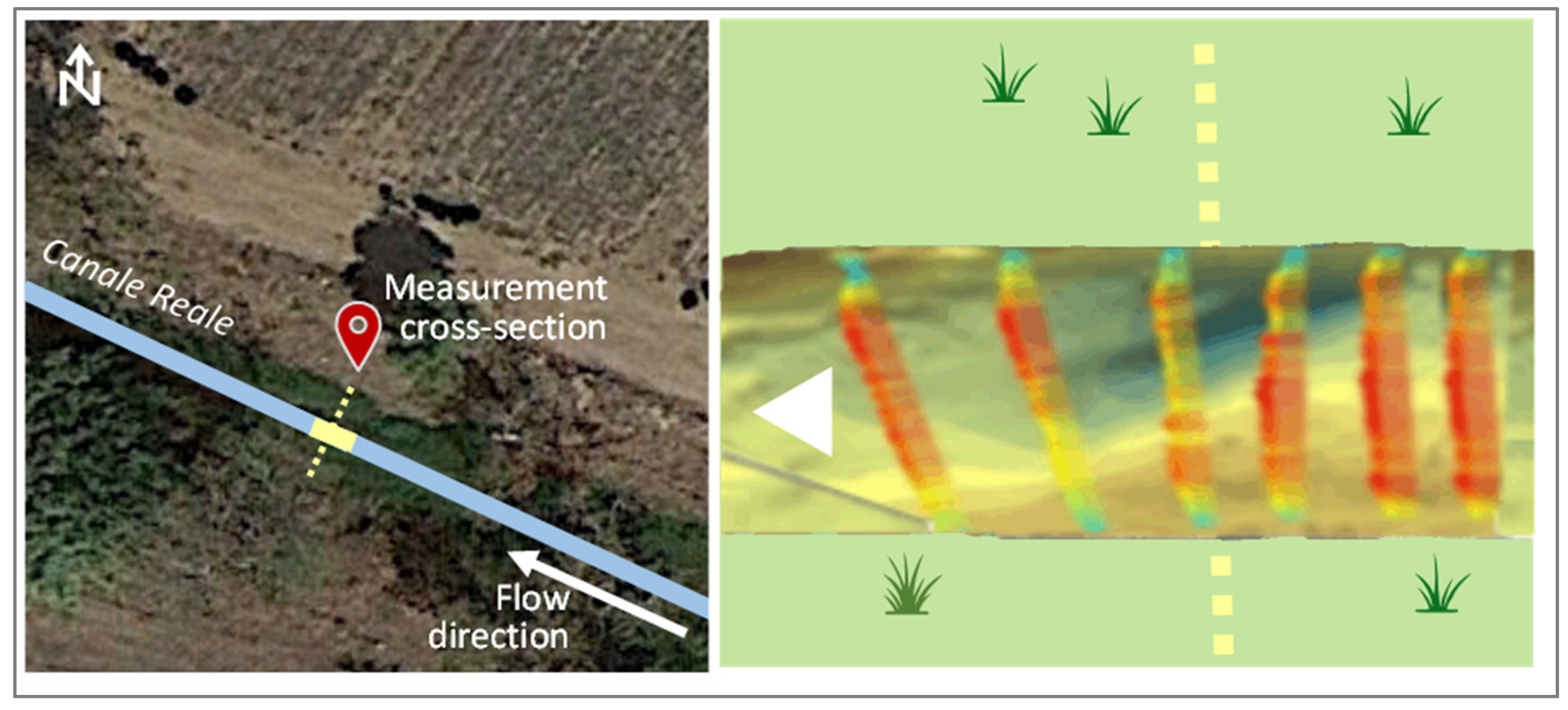
4.2. Field Flow Measurements and Method Validation

| On-Site Direct Measures | DAS Beamforming | |||
|---|---|---|---|---|
| Cross-Section | Wet Area (m2) | CM Method (L/s) | F Method (L/s) | Doppler (L/s) |
| A | 0.20 | 93.74 | 104 | 40 ÷ 280 |
| B1–B2 | 0.14 | 33.90 | nd | 28 ÷ 196 |
5. Conclusions
Author Contributions
Funding
Institutional Review Board Statement
Informed Consent Statement
Data Availability Statement
Conflicts of Interest
References
- Bradley, D.C.; Cadman, D.; Milner, N.J. Ecological Indicators of the Effects of Abstraction and Flow Regulation and Optimisation of Flow Releases from Water Storage Reservoirs. Project WFD21d Final Report SNIFFER, Edinburgh. 2012, pp. 1–261. Available online: https://www.wfduk.org/sites/default/files/Media/Assessing%20the%20status%20of%20the%20water%20environment/WFD21D%20Final%20Report_30%2008%2012.pdf (accessed on 8 February 2022).
- Rinaldi, M.; Belletti, B.; Van de Bund, W.; Bertoldi, W.; Gurnell, A.; Buijse, T.; Mosselman, E. Review on Eco-Hydromorphological Methods. Deliverable of the EU FP7 REFORM Project 2013. Available online: https://www.reformrivers.eu/system/files/1.1_REFORM_DeliverableD1.1_V8_Final.pdf (accessed on 8 February 2022).
- Sivapalan, M.; Takeuchi, K.; Franks, S.W.; Gupta, V.K.; Karambiri, H.; Lakshmi, V.; Liang, X.; McDonnell, J.J.; Mendiondo, E.M.; O’Connell, P.E.; et al. IAHS Decade on Predictions in Ungauged Basins (PUB), 2003–2012: Shaping an exciting future for the hydrological sciences. Hydrol. Sci. J. 2003, 48, 857–880. [Google Scholar] [CrossRef] [Green Version]
- Fiorentino, M.; Carriero, D.; Iacobellis, V.; Manfreda, S.; Portoghese, I. MEDCLUB-starting line and first activities. In Predictions in Ungauged Basins: Promises and Progress; Sivapalan, M., Wagener, T., Uhlenbrook, S., Zehe, E., Lakshmi, V., Liang, X., Tachikawa, Y., Kumar, P., Eds.; IAHS Press: Wallingford, UK, 2006; pp. 463–476. [Google Scholar]
- Sorman, A.U.; Abdulrazzak, M.J. Infiltration-recharge through wadi beds in arid regions. Hydrol. Sci. J. 2013, 38, 173–186. [Google Scholar] [CrossRef]
- Shentsis, I.; Rosenthal, E. Recharge of aquifers by flood events in an arid region. Hydrol. Processes 2003, 17, 695–712. [Google Scholar] [CrossRef]
- Niswonger, R.G.; Prudic, D.E. Documentation of the Streamflow-Routing (SFR2) Package to Include Unsaturated Flow Beneath Streams-A Modification to SFR1. US Geological Survey 2005. p. 51. Available online: https://pubs.usgs.gov/tm/2006/tm6A13/pdf/tm6a13.pdf (accessed on 8 February 2022).
- De Vries, J.J.; Simmers, I. Groundwater Recharge: An Overview of Processes and Challenges. Hydrogeol. J. 2002, 10, 5–17. [Google Scholar] [CrossRef]
- Scanlon, B.R.; Healy, R.W.; Cook, P.G. Choosing appropriate techniques for quantifying groundwater recharge. Hydrogeol. J. 2002, 10, 18–39. [Google Scholar] [CrossRef]
- Shanafield, M.; Cook, P.G. Transmission losses, infiltration and groundwater recharge through ephemeral and intermittent streambeds: A review of applied methods. J. Hydrol. 2014, 511, 518–529. [Google Scholar] [CrossRef]
- Abdulrazzak, M.J. Losses of flood water from alluvial channels. Arid. Soil Res. Rehabil. 1995, 9, 15–24. [Google Scholar] [CrossRef]
- Constantz, J.; Thomas, C.L. Stream bed temperature profiles as indicators of percolation characteristics beneath arroyos in the middle Rio Grande Basin, USA. Hydrol. Processes 1997, 11, 1621–1634. [Google Scholar] [CrossRef]
- Lay-Ekuakille, A.; Ugwiri, M.A.; Telesca, V.; Velazquez, R.; Passarella, G.; Maggi, S. Detection of river flow slow-down through sensing system and quasi-real time imaging. Flow Meas. Instrum. 2021, 81, 102042. [Google Scholar] [CrossRef]
- Lay-Ekuakille, A.; Okitadiowo, J.D.; Avoci Ugwiri, M.; Maggi, S.; Masciale, R.; Passarella, G. Video-Sensing Characterization for Hydrodynamic Features: Particle Tracking-Based Algorithm Supported by a Machine Learning Approach. Sensors 2021, 21, 4197. [Google Scholar] [CrossRef] [PubMed]
- Hamdhani, H.; Eppehimer, D.E.; Bogan, M.T. Release of treated effluent into streams: A global review of ecological impacts with a consideration of its potential use for environmental flows. Freshw. Biol. 2020, 65, 1657–1670. [Google Scholar] [CrossRef]
- Lay Ekuakille, A.; Vendramin, G.; Trotta, A. Beamforming-aided processing of EEG signals for analyzing epileptic seizures. Int. J. Adv. Media Commun. 2009, 3, 110–125. [Google Scholar] [CrossRef]
- Vergallo, P.; Lay-Ekuakille, A.; Giannoccaro, N.I.; Massaro, A.; Urooj, S.; Caratelli, D.; Trabacca, A. Processing EEG Signals through Beamforming Techniques for Seizure Diagnosis. In Proceedings of the 6th International Conference on Sensing Technology, Kolkata, India, 18–22 December 2012. [Google Scholar]
- Lay Ekuakille, A.; Vendramin, G.; Trotta, A. Beamforming-Based Acoustic Imaging for Distance Retrieval. In Proceedings of the 2008: IEEE International Instrumentation and Measurement Technology Conference, Victoria, BC, Canada, 12–15 May 2008; pp. 1466–1470. [Google Scholar]
- Warnick, K.F.; Maaskant, R.; Ivashina, M.V.; Davidson, D.B.; Jeffs, B.D. Phased Arrays for Radio Astronomy, Remote Sensing, and Satellite Communications; Cambridge University Press: Cambridge, UK, 2018; pp. 179–220, 253–299. [Google Scholar]
- Kumar, P.; Singhal, A.; Mehta, S.; Mittal, A. Real-time moving object detection algorithm on high-resolution videos using GPUs. J. Real-Time Image Process. 2016, 11, 93–109. [Google Scholar] [CrossRef]
- Monzingo, R.A.; Haupt, R.L.; Miller, T.W. Introduction to Adaptive Arrays; SciTech Pub. Inc.: Raleigh, NC, USA, 2011; p. 544. [Google Scholar]
- Suess, M.; Zubler, M.; Zahn, R. Performance investigation on the high resolution, wide swath SAR system. In Proceedings of the EUSAR, Cologne, Germany, 4–6 June 2002; pp. 187–191. [Google Scholar]
- Lay-Ekuakille, A.; Vendramin, G.; Trotta, A. Implementation and characterization of a novel acoustic imaging through beamformers for automotive applications. In Smart Sensors and Sensing Technology; Springer: Berlin/Heidelberg, Germany, 2008; Volume 20, pp. 343–359. [Google Scholar]
- Rad, A.G.; Dehghani, A.; Karim, M.R. Vehicle speed detection in video image sequences using CVS method. Int. J. Phys. Sci. 2010, 5, 2555–2563. [Google Scholar]
- Devendra, M.; Manjunathachari, K. DOA estimation of a system using MUSIC method. In Proceedings of the International Conference on Signal Processing and Communication Engineering Systems, Guntur, India, 2–3 January 2015; pp. 309–313. [Google Scholar]
- Lay-Ekuakille, A.; Giannoccaro, N.; Casciaro, S.; Conversano, F.; Velazquez, R. Modeling and Designing a Full Beamformer for Acoustic Sensing and Measurement. Int. J. Smart Sens. Intell. Syst. 2017, 10, 718–734. [Google Scholar] [CrossRef] [Green Version]
- Gupta, P.; Kar, S. MUSIC and improved MUSIC algorithm to estimate direction of arrival. In Proceedings of the International Conference on Communications and Signal Processing (ICCSP), Melmaruvathur, India, 2–4 April 2015; pp. 0757–0761. [Google Scholar]
- Lay-Ekuakille, A.; Vergallo, P.; Saracino, D.; Trotta, A. Optimizing and Post Processing of a Smart Beamformer for Obstacle Retrieval. IEEE Sens. J. 2012, 12, 1294–1299. [Google Scholar] [CrossRef]
- Al Ardi, E.M.; Shubair, R.M.; Al Mualla, M.E. Computationally Efficient High-Resolution DOA Estimation in a Multipath Environment. IEEE Electron. Lett. 2004, 40, 908–909. [Google Scholar]
- Mvemba, P.K.; Lay-Ekuakille, A.; Kidiamboko, S.; Zia Uhr Rahman, M. An Embedded Beamformer for a Pid Based-Trajectory Sensing Autonomous Vehicle. Metrol. Meas. Syst. 2018, 25, 561–575. [Google Scholar]
- Singh, S.; Chawla, R.; Singh, H. Intelligent speed violation detection system. Int. J. Eng. Res. Technol. 2014, 2, 92–95. [Google Scholar]
- Abbass, A. Estimating vehicle speed using image processing. Al-Mansour J. 2010, 14, 127–140. [Google Scholar]
- Crocco, M.; Trucco, A. The synthesis of robust broadband beamformers for equally-spaced linear arrays. J. Acoust. Soc. Am. 2020, 128, 691–701. [Google Scholar] [CrossRef] [PubMed]
- Yardibi, T.; Li, J.; Stoica, P. Nonparametric and sparse signal representations in array processing via iterative adaptive approaches. In Proceedings of the 42nd Asilomar Conference on Signals, Systems and Computers, Pacific Grove, CA, USA, 26–29 October 2008; pp. 278–282. [Google Scholar]
- Chen, W.; Zhao, Y.; Gao, J. Improved capon beamforming algorithm by using inverse covariance matrix calculation. In Proceedings of the IET International Radar Conference, Xi’an, China, 4–16 April 2013; pp. 1–6. [Google Scholar]
- Krieger, G.; Gebert, N.; Moreira, A. Multidimensional Waveform Encoding: A New Digital Beamforming Technique for Synthetic Aperture Radar Remote Sensing. IEEE Trans. Geosci. Remote Sens. 2008, 46, 31–46. [Google Scholar] [CrossRef] [Green Version]
- Ciaranfi, N.; Pieri, P.; Ricchetti, G. Note alla carta geologica delle Murge e del Salento (Puglia Centro Meridionale). Mem. Soc. Geol. Ital. 1988, 41, 449–460. [Google Scholar]
- Spizzico, M.; Lopez, N.; Sciannamblo, D. Analysis of the potential contamination risk of groundwater resources circulating in areas with anthropogenic activities. Nat. Hazards Earth Syst. Sci. 2005, 5, 109–116. [Google Scholar] [CrossRef]
- Tozzi, M. Assetto tettonico dell’avampaese apulo meridionale (Murge meridionali-Salento) sulla base di dati strutturali. Geol. Rom. 1993, 29, 95–111. [Google Scholar]
- Maggiore, M.; Pagliarulo, P. Circolazione idrica ed equilibri idrogeologici negli acquiferi della Puglia. Geol. Territ. 2004, 1, 13–35. [Google Scholar]
- Sciannamblo, D.; Spizzico, M.; Tadolini, T.; Tinelli, R. Lineamenti idrogeologici della zona umida di Torre Guaceto (Br). Geol. Rom. 1994, 30, 754–760. [Google Scholar]
- Masciale, R.; Amalfitano, S.; Frollini, E.; Ghergo, S.; Melita, M.; Parrone, D.; Passarella, G. Assessing natural background levels in the groundwater bodies of the Apulia Region (Southern Italy). Water 2021, 13, 958. [Google Scholar] [CrossRef]
- Lo Presti, R.; Barca, E.; Passarella, G. A methodology for treating missing data applied to daily rainfall data in the Candelaro River Basin (Italy). Environ. Monit. Assess. 2010, 160, 1. [Google Scholar] [CrossRef]
- Passarella, G.; Bruno, D.; Lay-Ekuakille, A.; Maggi, S.; Masciale, R.; Zaccaria, D. Spatial and temporal classification of coastal regions using bioclimatic indices in a Mediterranean environment. Sci. Total Environ. 2020, 700, 134415. [Google Scholar] [CrossRef]
- Maggi, S.; Bruno, D.; Lay-Ekuakille, A.; Masciale, R.; Passarella, G. Automatic processing of bioclimatic data in the space and time domains. J. Phys. Conf. Ser. 2018, 1065, 192005. [Google Scholar] [CrossRef] [Green Version]
- Passarella, G.; Barca, E.; Bruno, D.E.; Maggi, S.; Masciale, R.; Lay-Ekuakille, A. Accurate classification of bioclimatic data: Spatial analysis. In Proceedings of the EnvIMEKO 17—7th IMEKO TC19 Symposium on Environmental Instrumentation and Measurements, Aguascalientes, Mexico, 3–4 August 2017; Available online: https://www.imeko.org/publications/tc19-2017/IMEKO-TC19-2017-016.pdf (accessed on 8 February 2022).
- Passarella, G.; Barca, E.; Bruno, D.E.; Maggi, S.; Masciale, R.; Lay-Ekuakille, A. Accurate classification of bioclimatic data: Temporal analysis. In Proceedings of the EnvIMEKO 17—7th IMEKO TC19 Symposium on Environmental Instrumentation and Measurements, Aguascalientes, Mexico, 3–4 August 2017; Available online: https://www.imeko.org/publications/tc19-2017/IMEKO-TC19-2017-018.pdf (accessed on 8 February 2022).
- Mann, H.B. Nonparametric tests against trend. Econometrica 1945, 13, 245–259. [Google Scholar] [CrossRef]
- Yue, S.; Pilon, P.; Cavadias, G. Power of Mann-Kendall and Spearman’s rho tests for detecting monotonic trends in hydrological series. J. Hydrol. 2002, 259, 254–271. [Google Scholar] [CrossRef]
- Brouwer, C.; Heibloem, M. Irrigation water management: Irrigation water needs. Train. Man. 1986, 3, 1–103. Available online: https://www.fao.org/3/s2022e/s2022e00.htm#Contents (accessed on 8 February 2022).
- Hargreaves, G.H.; Samani, Z.A. Estimating potential evapotranspiration. J. Irrig. Drain. Div. 1982, 108, 225–230. [Google Scholar] [CrossRef]
- Apulian Civil Protection. Hydrological Annals. Available online: https://protezionecivile.puglia.it/ (accessed on 8 February 2022).
- Zaccaria, D.; Passarella, G.; D’Agostino, D.; Giordano, R.; Sandoval-Solis, S. Risk Assessment of Aquifer Salinization in a Large-Scale Coastal Irrigation Scheme, Italy. Clean-Soil Air Water 2016, 44, 371–382. [Google Scholar] [CrossRef]
- Doglioni, A.; Simeone, V. Effects of Climatic Changes on Groundwater Availability in a Semi-arid Mediterranean Region. In IAEG/AEG Annual Meeting Proceedings, San Francisco, California; Shakoor, A., Cato, K., Eds.; Springer: Cham, Switzerland, 2019; Volume 4, pp. 105–110. [Google Scholar]
- Dobriyal, P.; Badola, R.; Tuboi, C.; Husain, S.A. A review of methods for monitoring streamflow for sustainable water resource management. Appl. Water Sci. 2017, 7, 2617–2628. [Google Scholar] [CrossRef] [Green Version]
- Portoghese, I.; Masciale, R.; Caputo, M.C.; De Carlo, L.; Malcangio, D. Combined Discharge and Thermo-Salinity Measurements for the Characterization of a Karst Spring System in Southern Italy. Sustainability 2020, 12, 3311. [Google Scholar] [CrossRef] [Green Version]
- World Meteorological Organization. Guide to Hydrological Practices Vol. I: Hydrology—From Measurement to Hydrological Information, 6th ed.; WMO No.168; World Meteorological Organization: Geneva, Switzerland, 2008; Available online: https://library.wmo.int/doc_num.php?explnum_id=10473 (accessed on 8 February 2022).
- Herschy, R.W. Streamflow Measurement, 3rd ed.; CRC Press: London, UK, 2008; p. 536. [Google Scholar]


Publisher’s Note: MDPI stays neutral with regard to jurisdictional claims in published maps and institutional affiliations. |
© 2022 by the authors. Licensee MDPI, Basel, Switzerland. This article is an open access article distributed under the terms and conditions of the Creative Commons Attribution (CC BY) license (https://creativecommons.org/licenses/by/4.0/).
Share and Cite
Passarella, G.; Lay-Ekuakille, A.; Djungha Okitadiowo, J.P.; Masciale, R.; Brigida, S.; Matarrese, R.; Portoghese, I.; Isernia, T.; Blois, L. An Affordable Streamflow Measurement Technique Based on Delay and Sum Beamforming. Sensors 2022, 22, 2843. https://doi.org/10.3390/s22082843
Passarella G, Lay-Ekuakille A, Djungha Okitadiowo JP, Masciale R, Brigida S, Matarrese R, Portoghese I, Isernia T, Blois L. An Affordable Streamflow Measurement Technique Based on Delay and Sum Beamforming. Sensors. 2022; 22(8):2843. https://doi.org/10.3390/s22082843
Chicago/Turabian StylePassarella, Giuseppe, Aimé Lay-Ekuakille, John Peter Djungha Okitadiowo, Rita Masciale, Silvia Brigida, Raffaella Matarrese, Ivan Portoghese, Tommaso Isernia, and Luciano Blois. 2022. "An Affordable Streamflow Measurement Technique Based on Delay and Sum Beamforming" Sensors 22, no. 8: 2843. https://doi.org/10.3390/s22082843
APA StylePassarella, G., Lay-Ekuakille, A., Djungha Okitadiowo, J. P., Masciale, R., Brigida, S., Matarrese, R., Portoghese, I., Isernia, T., & Blois, L. (2022). An Affordable Streamflow Measurement Technique Based on Delay and Sum Beamforming. Sensors, 22(8), 2843. https://doi.org/10.3390/s22082843