
Quantification and Visualization of Reliable Hemodynamics Evaluation Based on Non-Contact Arteriovenous Fistula Measurement

 , , , , , ,
Abstract
:1. Introduction
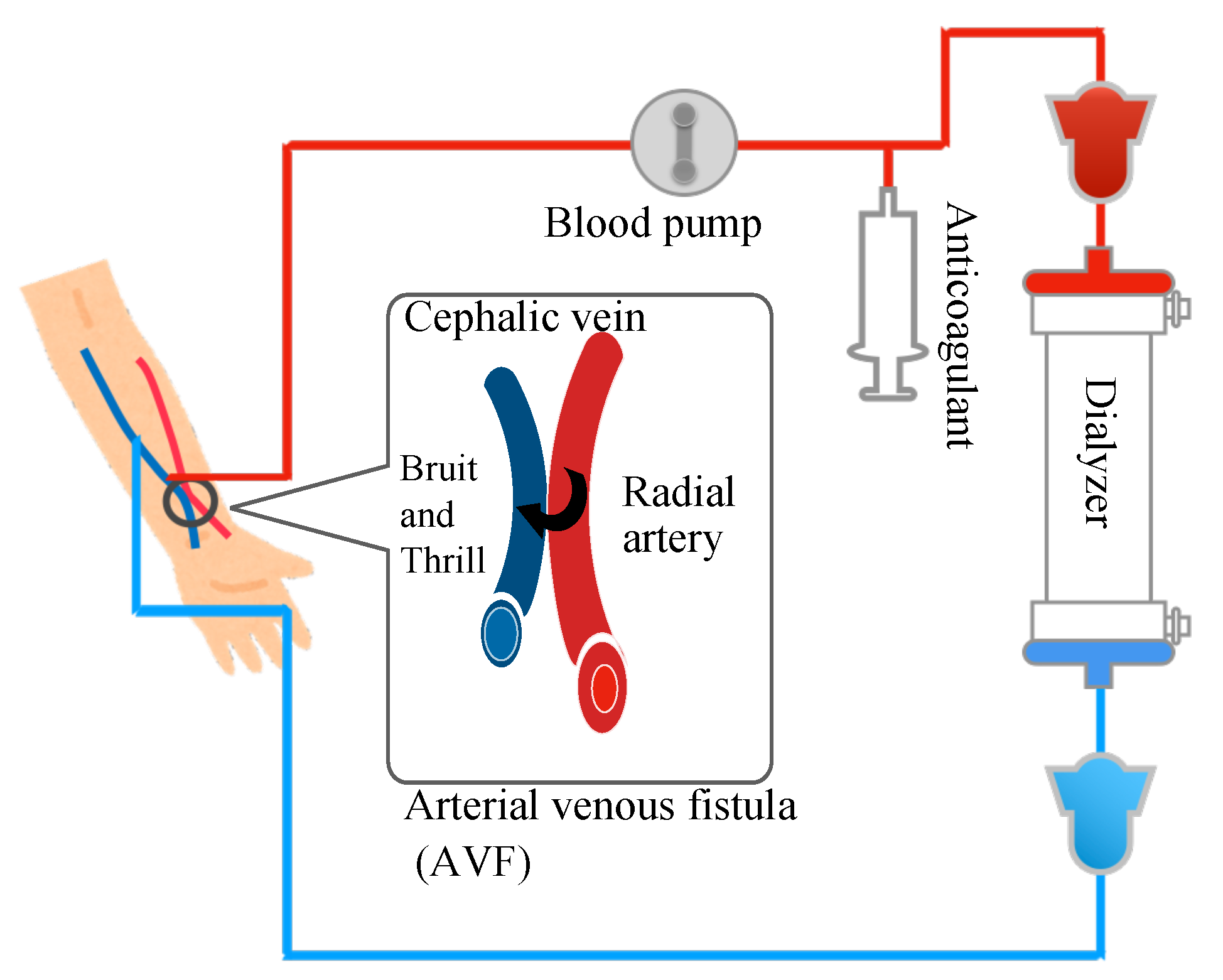
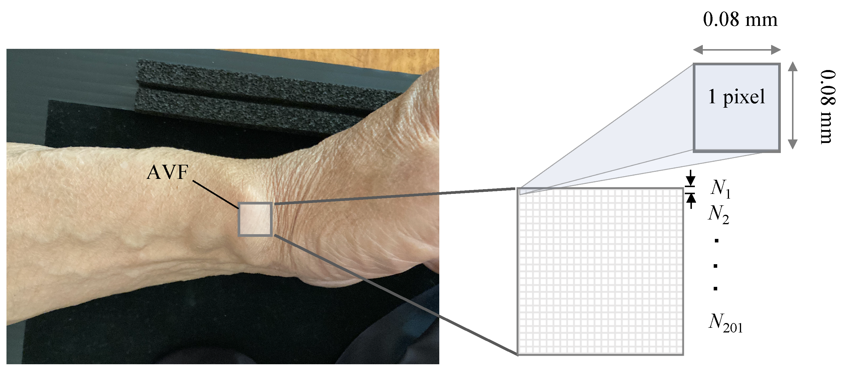
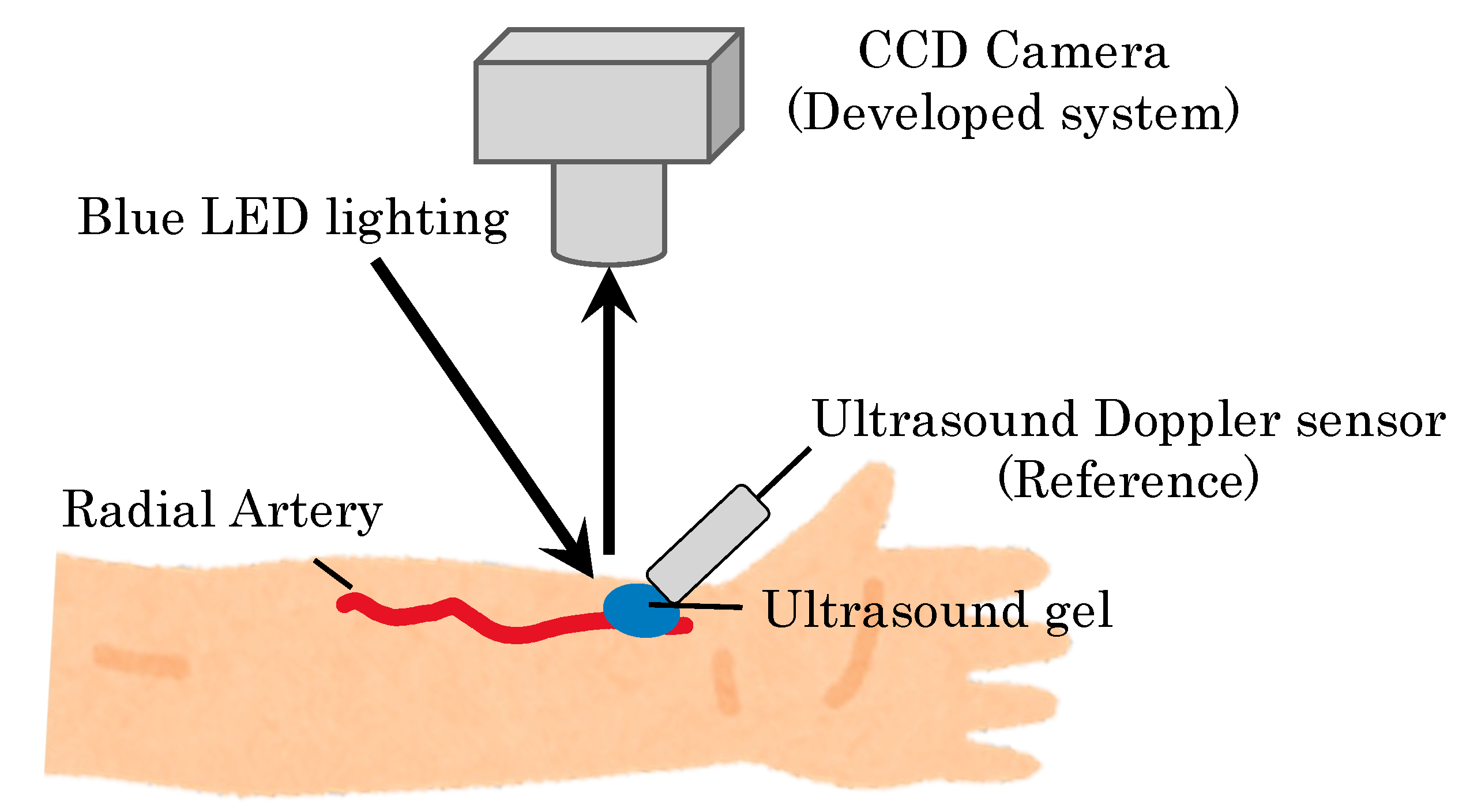
2. Principle of Non-Contact AVF Pulse Wave Measurement
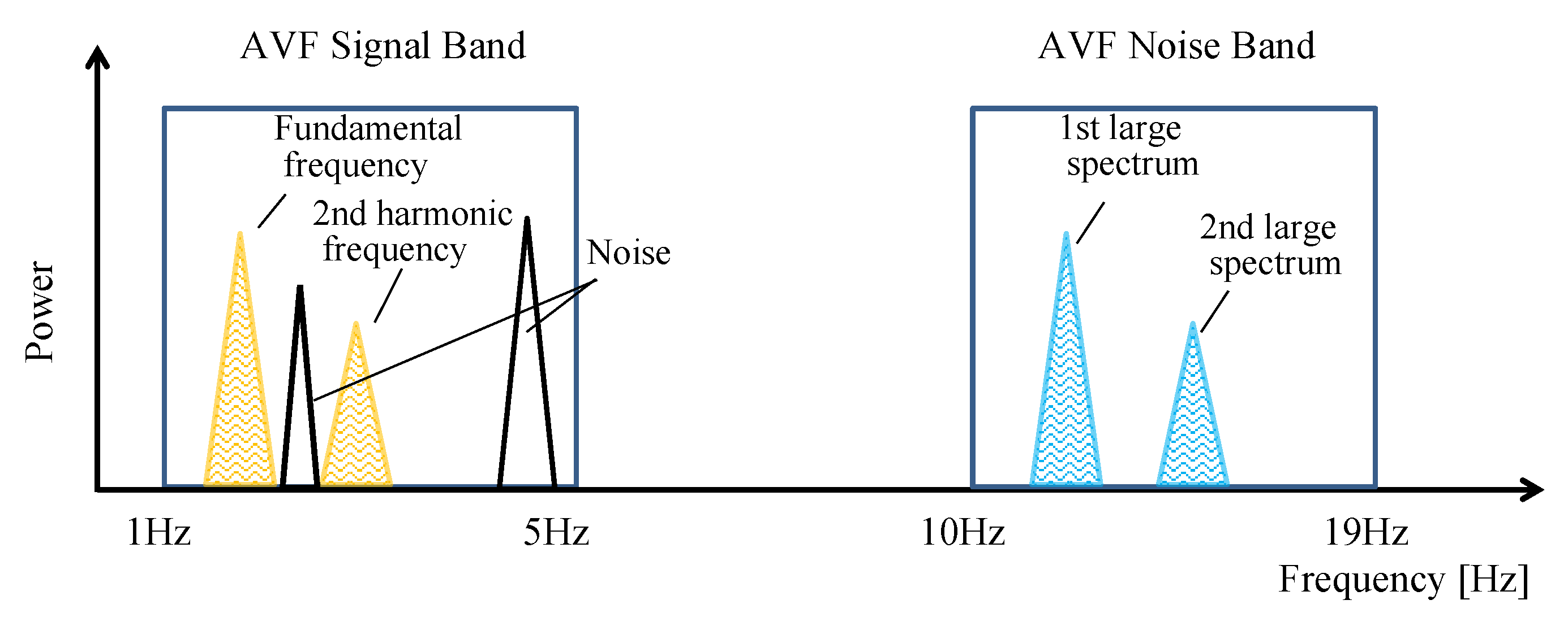
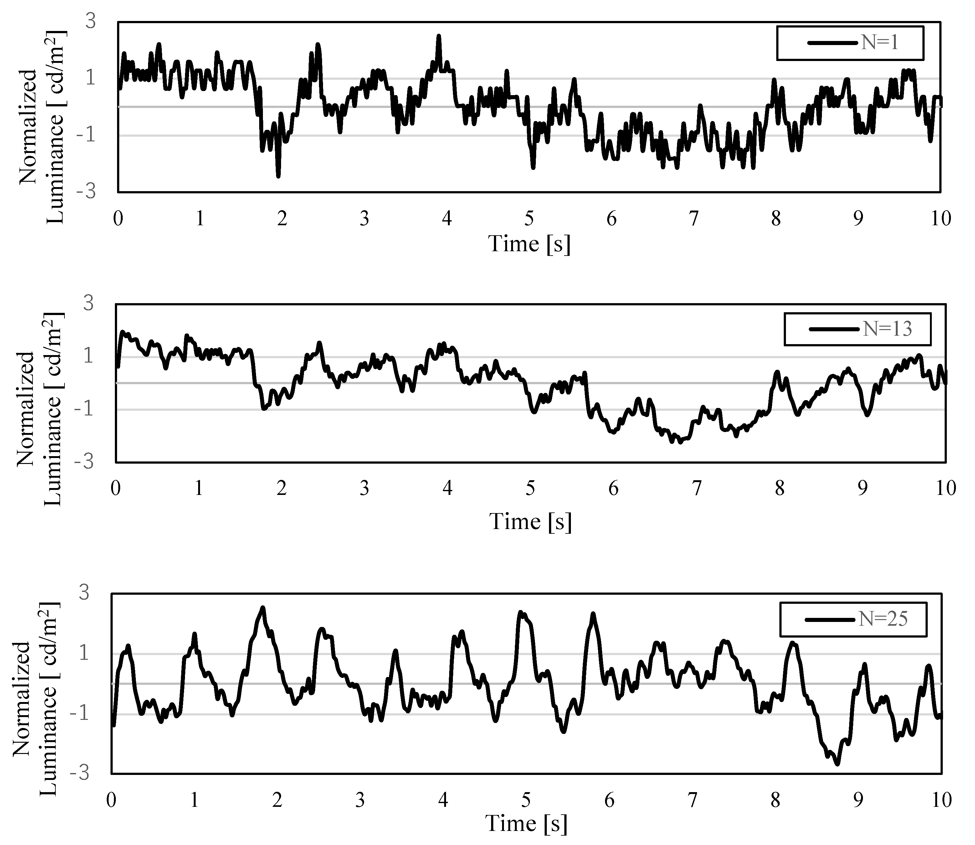
Moving-Average Filter
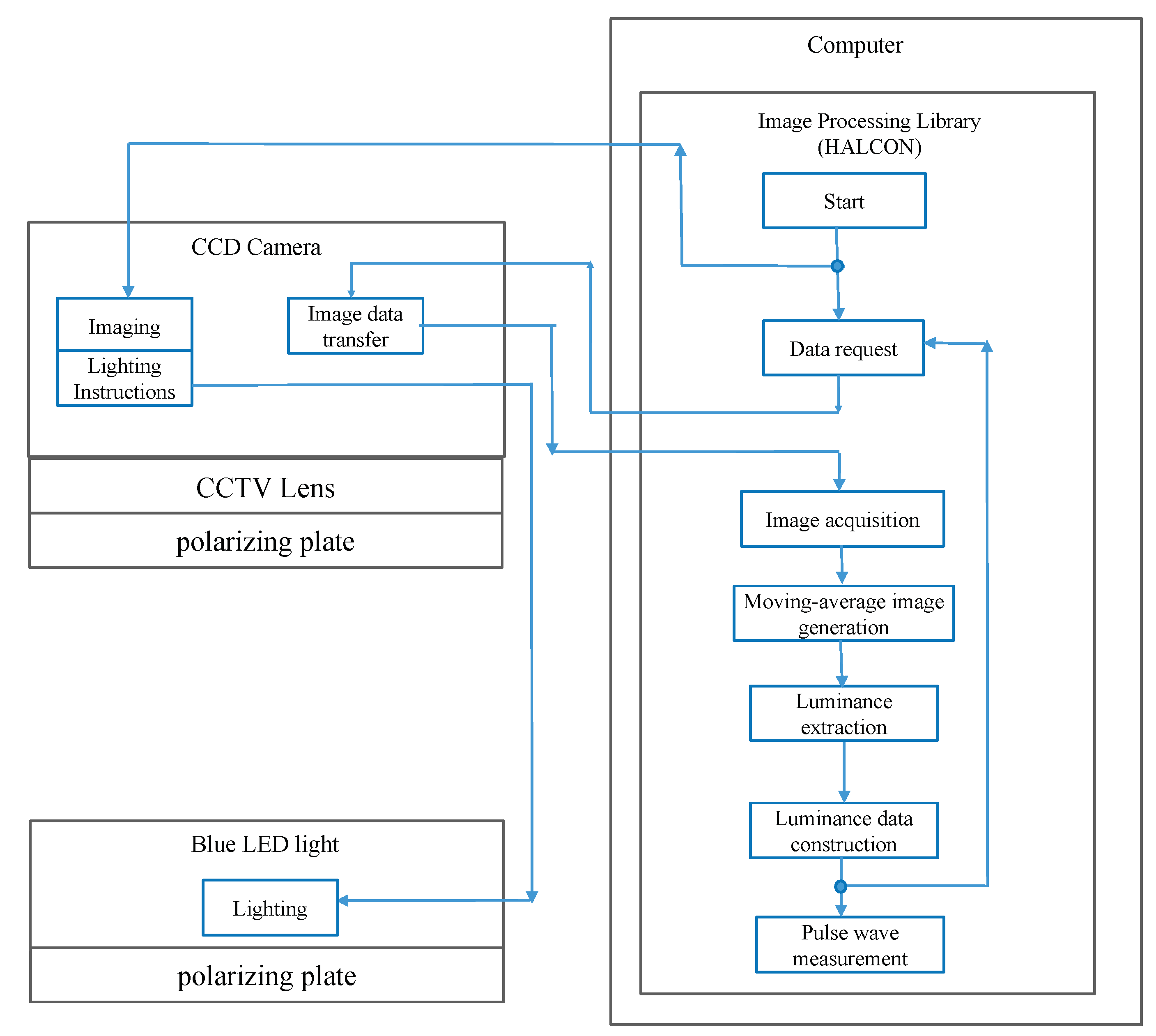
3. Methods
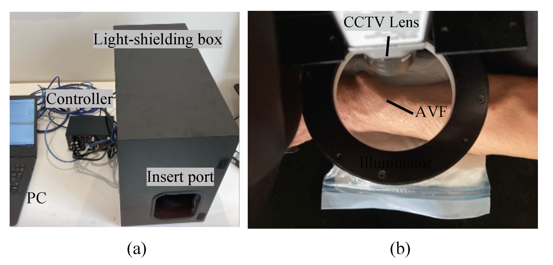
3.1. Experimental Protocol
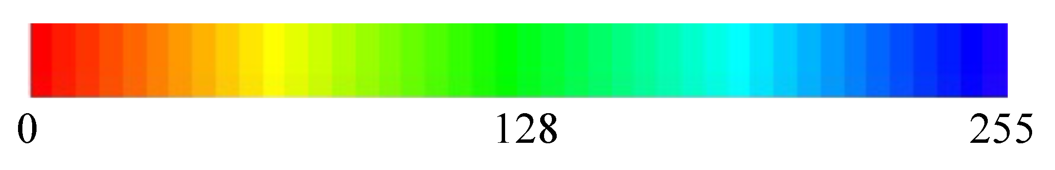
3.2. Hemodynamics Visualization Method Based on Color Mapping
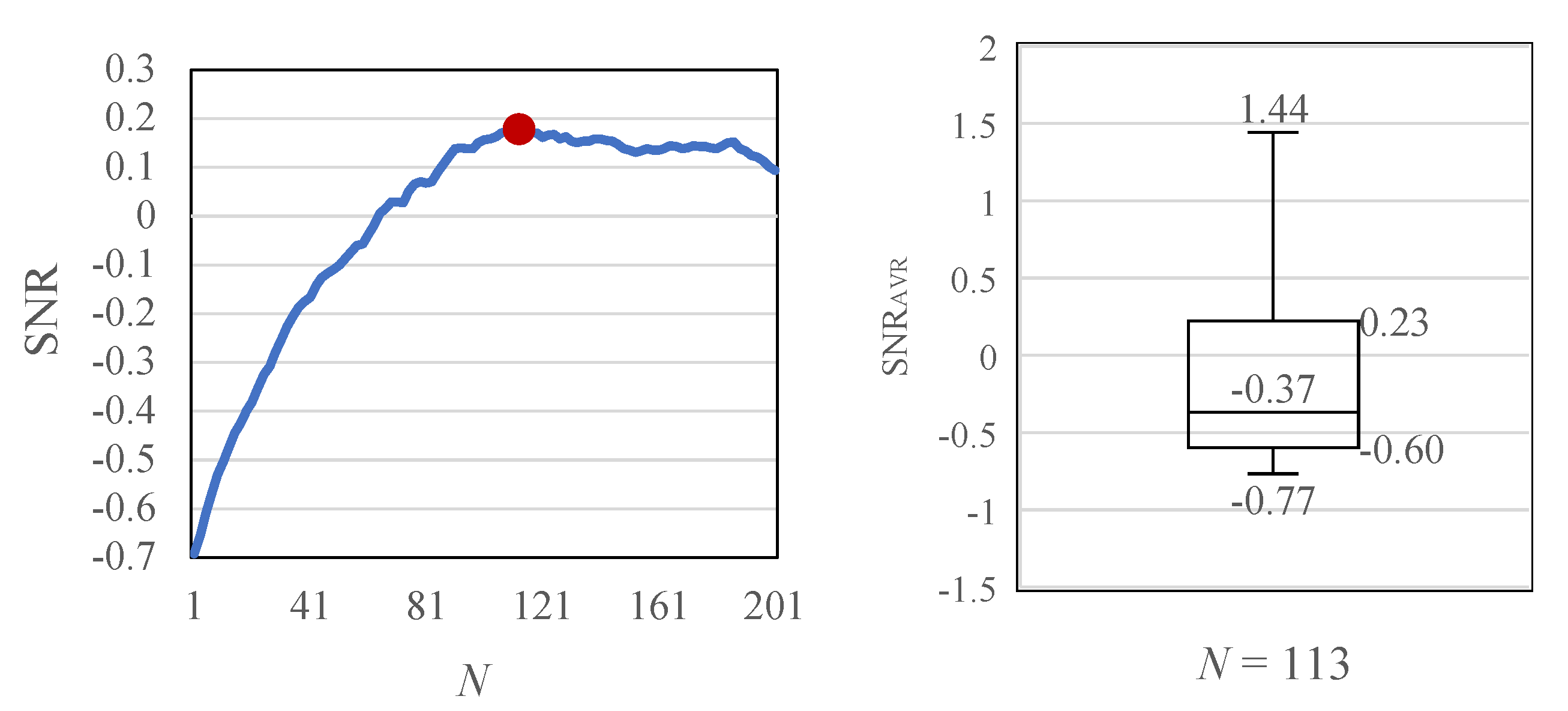
3.3. Determination of the Optimal Kernel Size and Quantification
4. Results
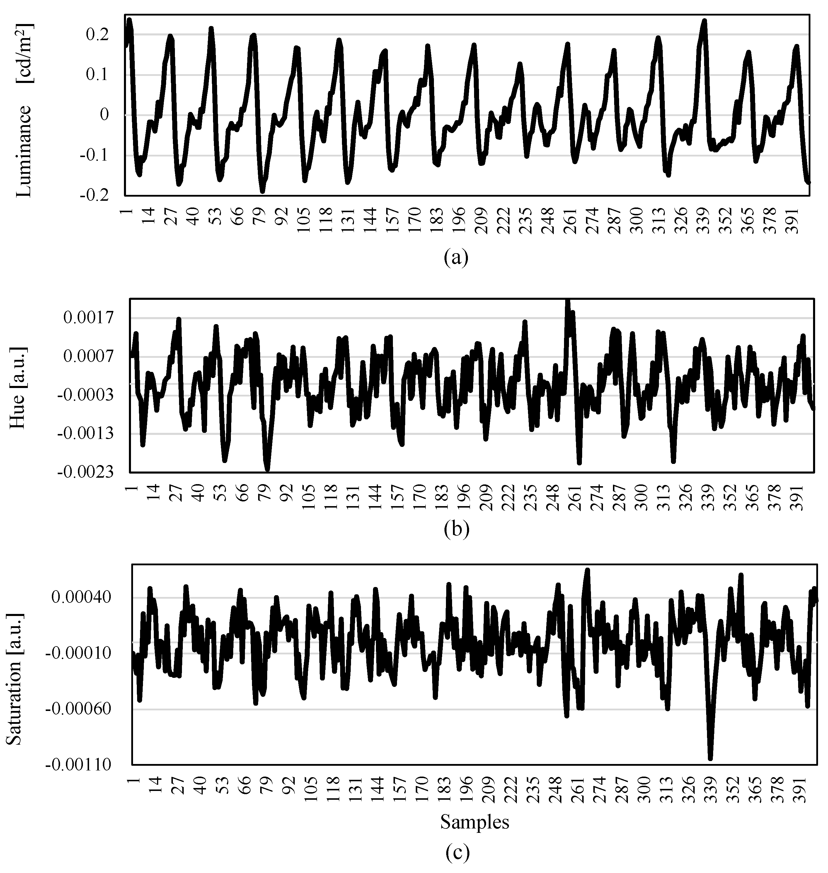
4.1. Preliminary Evaluation: Effect of Changes in Luminance, Hue, and Color Saturation on Pulse Waveform
4.2. Preliminary Evaluation: Optimal Wavelength of Imaging
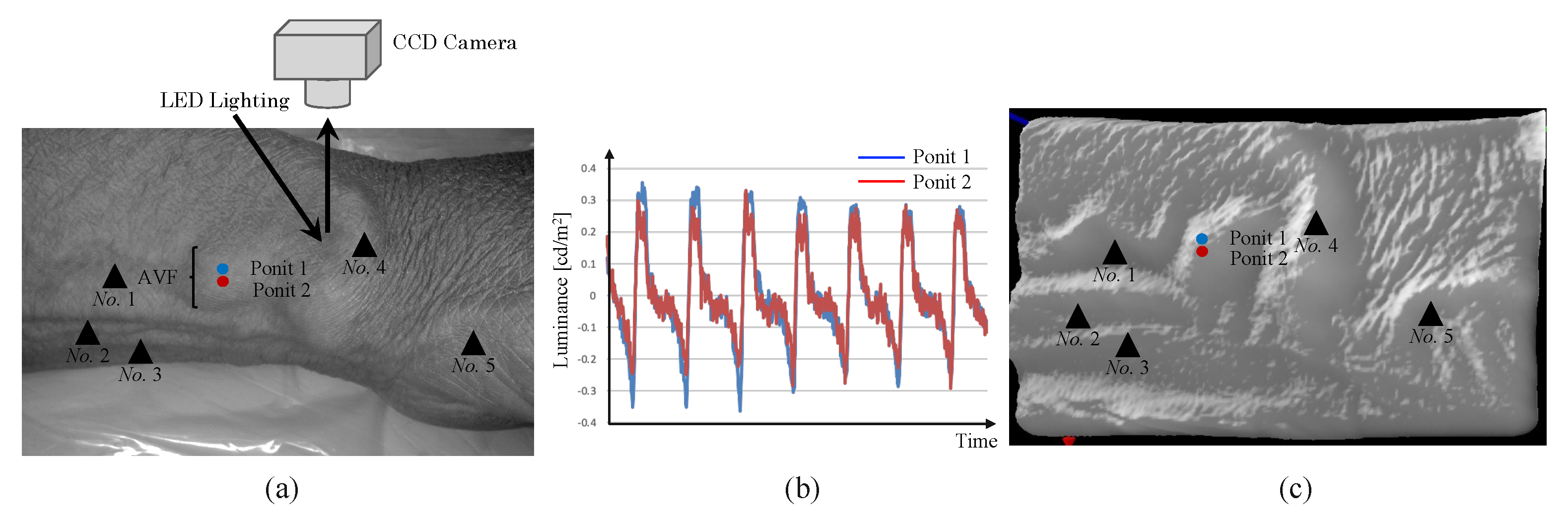
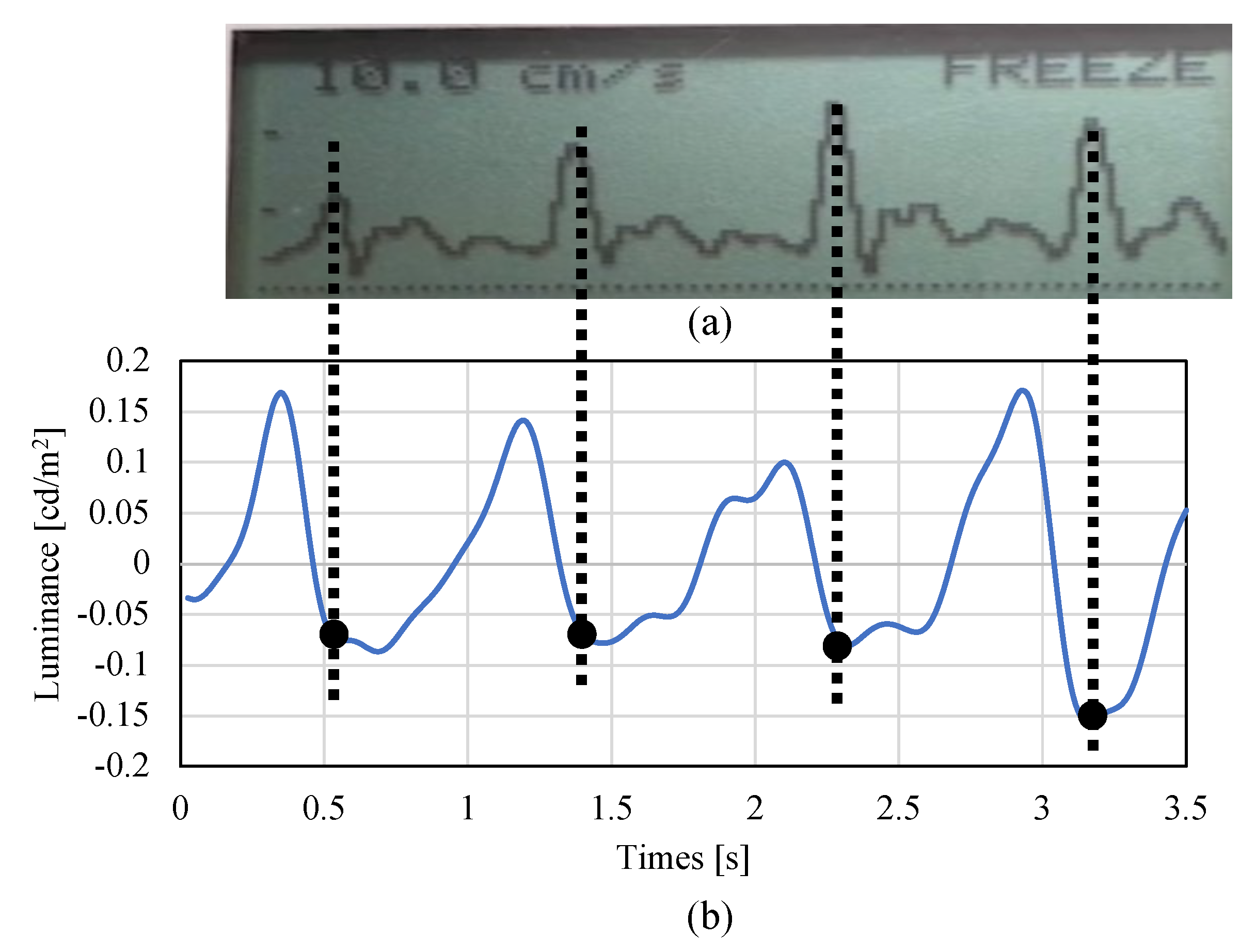
4.3. Preliminary Evaluation: Validation of Non-Contact AVF Imaging
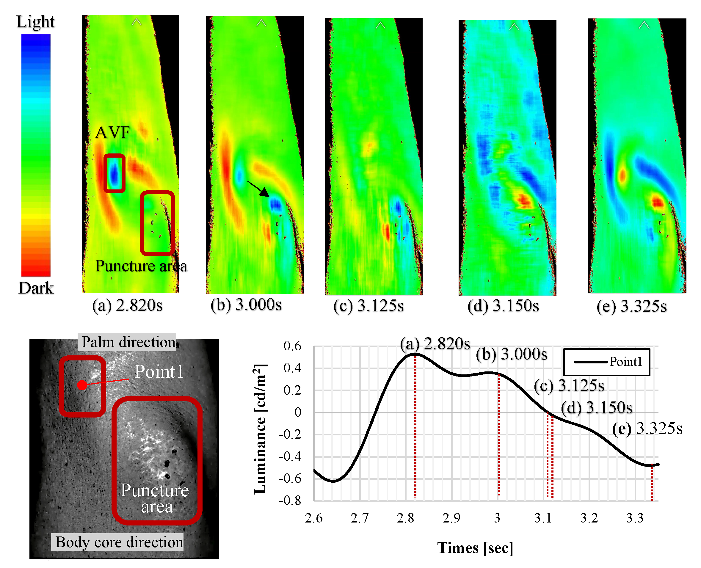
4.4. Color Mapping-Based Hemodynamic Visualization
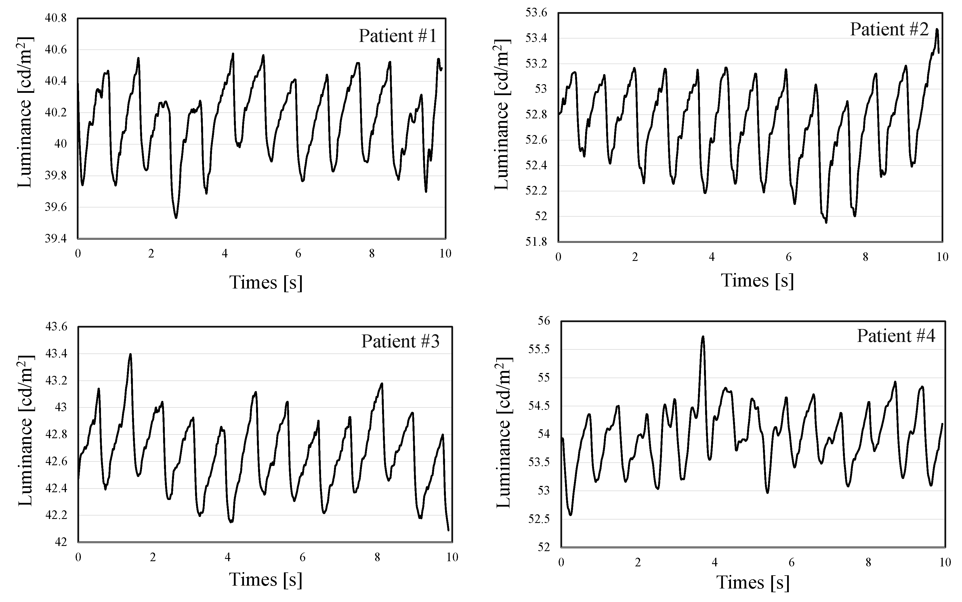
4.5. Measurement Data with Moving-Average Filtering
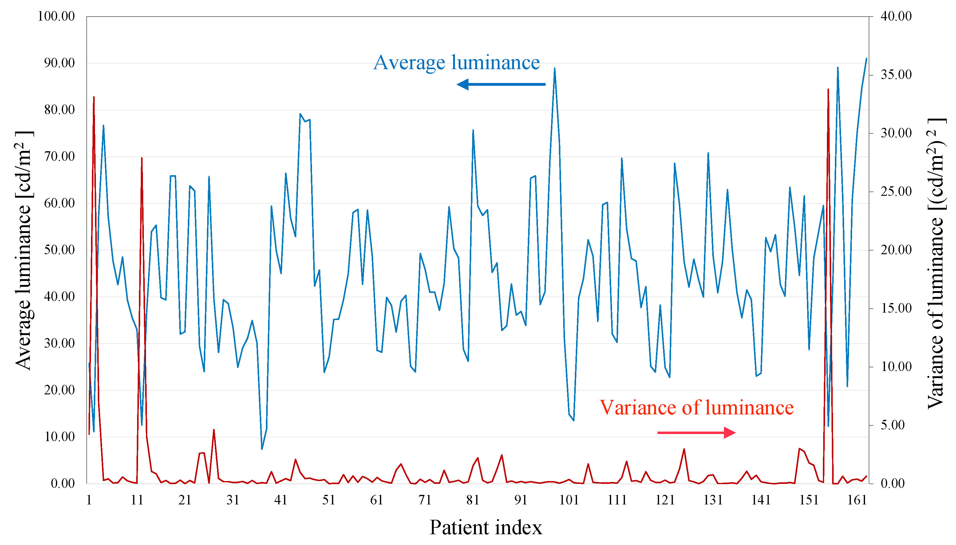
4.6. AVF Quantification with Optimal Kernel Size
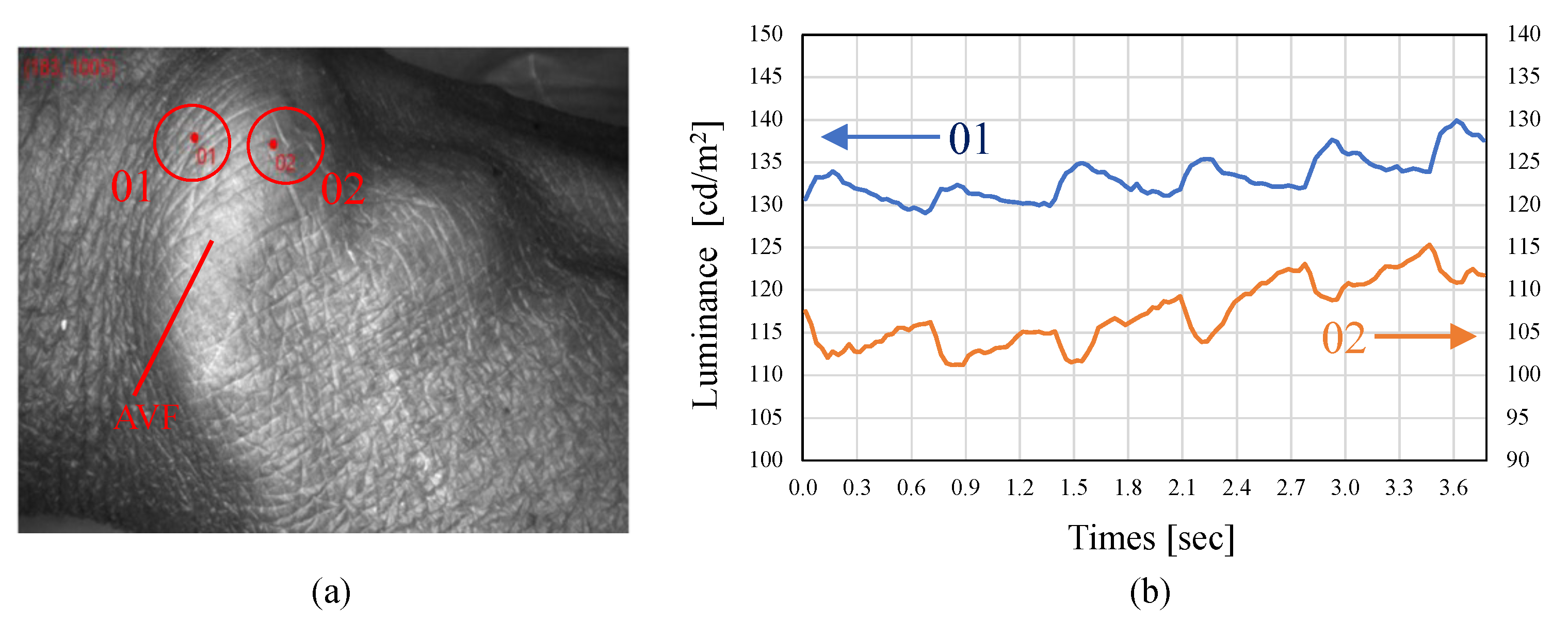
4.7. Observation of the Reversed-Phase Pulse Wave
5. Discussion
5.1. Visualization by Color Mapping
5.2. AVF Pulse Wave and Stereoscopic Image with Blue Light
5.3. Effect of Moving-Average Filtering
5.4. Limitation of Developed Non-Contact AVF Evaluation System
6. Conclusions
Author Contributions
Funding
Institutional Review Board Statement
Informed Consent Statement
Conflicts of Interest
Abbreviations
| AVF | Arteriovenous Fistula |
| BPF | Band-Pass Filter |
| CCD | Charge-Coupled Device |
| FFT | Fast Fourier Transform |
| PPG | Photoplethysmography |
| SNR | Signal-to-Noise power Ratio |
References
- Fresenius Medical Care Annual Report 2020. Available online: https://www.freseniusmedicalcare.com/fileadmin/data/com/pdf/Media_Center/Publications/Annual_Reports/FME_Annual_Report_2020_EN.pdf (accessed on 24 January 2022).
- Nitta, K.; Masakane, I.; Nakai, S.; Ogata, S.; Kimata, N.; Hanafusa, N.; Hamano, T. 2019 annual dialysis data report, JSDT renal data registry. J. Jpn. Soc. Dialysis Ther. 2020, 53, 579–632. [Google Scholar] [CrossRef]
- Corada, M.; Morini, M.F.; Dejana, E. Signaling pathways in the specification of arteries and veins. Arterioscler. Thrombosis Vasc. Biol. 2014, 34, 2372–2377. [Google Scholar] [CrossRef]
- Ene–Iordache, B.; Semperboni, C.; Dubini, G.; Remuzzi, A. Disturbed flow in a patient-specific arteriovenous fistula for hemodialysis: Multidirectional and reciprocating near–wall flow patterns. J. Biomech. 2015, 48, 2195–2200. [Google Scholar] [CrossRef]
- Remuzzi, A.; Bozzetto, M. Biological and physical actors involved in the maturation of arteriovenous fistula for hemodialysis. Cardiovasc. Eng. Technol. 2017, 8, 273–279. [Google Scholar] [CrossRef]
- Pablo, V. AV fistula diagnosis procedures. In Acoustical Signal Processing of Arterio Venous Fistula Bruits; Department of Electrical and Information Technology, Lund University: Lund, Sweden, 2015; pp. 10–11. [Google Scholar]
- Wang, Y.N.; Chan, C.Y.; Chou, S.J. The detection of arteriovenous fistula stenosis for hemodialysis based on wavelet transform. Int. J. Adv. Comput. Sci. 2011, 1, 16–22. [Google Scholar]
- Panda, B.; Mandal, S.; Majerus, S. Vascular stenosis detection using temporal-spectral differences in correlated acoustic measurements. In Proceedings of the 2019 IEEE Signal Processing in Medicine and Biology Symposium, Philadelphia, PA, USA, 7 December 2019. [Google Scholar] [CrossRef]
- Sung, P.H.; Kan, C.D.; Chen, W.L.; Jang, L.S.; Wang, J.F. Hemodialysis vascular access stenosis detection using auditory spectro-temporal features of phonoangiography. Med. Biol. Eng. Comput. 2015, 53, 393–403. [Google Scholar] [CrossRef]
- Wang, H.; Wu, C.; Chen, C.; Lin, B. Novel noninvasive approach for detecting arteriovenous fistula stenosis. IEEE Trans. Biomed. Eng. 2014, 61, 1851–1857. [Google Scholar] [CrossRef]
- Chin, S.; Panda, B.; Damaser, M.S.; Majerus, S.J.A. Stenosis characterization and identification for dialysis vascular access. In Proceedings of the 2018 IEEE Signal Processing in Medicine and Biology Symposium, Philadelphia, PA, USA, 1 December 2018; pp. 1–5. [Google Scholar] [CrossRef]
- Gram, M.; Olesen, J.T.; Riis, H.C.; Selvaratnam, M.; Meyer-Hofmann, H.; Pedersen, B.B.; Schmidt, S.E. Stenosis detection algorithm for screening of arteriovenous fistulae. In Proceedings of the 15th Nordic-Baltic Conference on Biomedical Engineering and Medical Physics (NBC2011), Aalborg, Denmark, 14–17 June 2011; Springer: Berlin/Heidelberg, Fermany, 2011; pp. 241–244. [Google Scholar] [CrossRef]
- Ota, K.; Nishiura, Y.; Ishihara, S.; Adachi, H.; Yamamoto, Y.; Hamano, T. Evaluation of hemodialysis arteriovenous bruit by deep learning. Sensors 2020, 20, 4852. [Google Scholar] [CrossRef]
- Mansy, H.A.; Hoxie, S.J.; Patel, N.H.; Sandler, R.H. Computerised analysis of auscultatory sounds associated with vascular patency of haemodialysis access. Med. Biol. Eng. Comput. 2005, 43, 56–62. [Google Scholar] [CrossRef]
- Sato, T.; Tsuji, K.; Kawashima, N.; Agishi, T.; Toma, H. Evaluation of blood access dysfunction based on a wavelet transform analysis of shunt murmurs. J. Artif. Organs 2006, 9, 97–104. [Google Scholar] [CrossRef]
- Yi–Chun, D.; Stephanus, A. Levenberg–Marquardt neural network algorithm for degree of arteriovenous fistula stenosis classification using a dual optical photoplethysmography sensor. Sensors 2018, 18, 2322. [Google Scholar]
- Chiang, P.Y.; Chao, P.C.P.; Tu, T.Y.; Kao, Y.H.; Yang, C.Y.; Tarng, D.C.; Wey, C.L. Machine learning classification for assessing the degree of stenosis and blood flow volume at arteriovenous fistulas of hemodialysis patients using a new photoplethysmography sensor device. Sensors 2019, 19, 3422. [Google Scholar] [CrossRef] [Green Version]
- Kamiyama, H.; Kitama, M.; Shimizu, H.O.; Yamashita, M.; Kojima, Y.; Shimizu, K. Fundamental study for optical transillumination imaging of arteriovenous fistula. Adv. Biomed. Eng. 2021, 10, 1–10. [Google Scholar] [CrossRef]
- Zhu, F.; Williams, S.; Putnam, H.; Campos, I.; Johnson, C.; Kappel, F.; Kotanko, P. Estimation of arterio-venous access blood flow in hemodialysis patients using video image processing technique. In Proceedings of the 38th Annual International Conference of the IEEE Engineering in Medicine and Biology Society (EMBC2016), Orlando, FL, USA, 16–20 August 2016; pp. 207–210. [Google Scholar]
- Heckenlively, J.R.; Arden, G.B. Principles and Practice of Clinical Electrophysiology of Vision, 2nd ed.; MIT Press: Cambridge, MA, USA, 2006; p. 222. [Google Scholar]
- Kumar, A.; Bhattacharya, A.; Makhija, N. Evoked potential monitoring in anaesthesia and analgesia. Anaesthesia 2000, 55, 225–241. [Google Scholar] [CrossRef]
- Monroe, L. Physical Rehabilitation for the Physical Therapist Assistant, 1st ed.; Elsevier Health Sciences: Amsterdam, The Netherlands, 2014; p. 347. [Google Scholar]
- Shimazaki, T.; Hara, S.; Okuhata, H.; Nakamura, H.; Kawabata, T. Heart rate sensing during exercise by means of photoplethysmography. Trans. Jpn. Soc. Med. Biol. Eng. 2017, 54, 225–235. [Google Scholar]
- Logvinenko, A.D. The geometric structure of color. J. Vision Jan. 2015, 15, 16. [Google Scholar] [CrossRef] [PubMed]
- Spigulis, J.; Gailite, L.; Lihachev, A.; Erts, R. Simultaneous recording of skin blood pulsations at different vascular depths by multiwavelength Photoplethysmography. Appl. Opt. 2007, 46, 1754–1759. [Google Scholar] [CrossRef] [Green Version]
- Maeda, Y.; Sekine, M.; Tamura, T. Relationship between measurement site and motion artifacts in wearable reflected photoplethysmography. J. Med. Syst. 2011, 35, 969–976. [Google Scholar] [CrossRef]
- Shimazaki, T.; Hara, S.; Okuhata, H.; Nakamura, H.; Kawabata, T. Cancellation of motion artifact induced by exercise for PPG-based heart rate sensing. In Proceedings of the 36th Annual International Conference of the IEEE Engineering in Medicine and Biology Society (EMBC2014), Chicago, IL, USA, 26–30 August 2014; pp. 3216–3219. [Google Scholar] [CrossRef]
- Simazaki, T.; Anzai, D.; Watanabe, K.; Nakajima, A.; Fukuda, M.; Ata, S. Heat stroke prevention in hot specific occupational environment enhanced by supervised machine learning with personalized vital signs. Sensors 2022, 22, 395. [Google Scholar] [CrossRef]
- Woodham, R.J. Photometric method for determining surface orientation from multiple images. Opt. Eng. 1980, 19, 139–144. [Google Scholar] [CrossRef]
- Santo, H.; Samejima, M.; Sugano, Y.; Shi, B.; Matsushita, Y. Deep photometric stereo networks for determining surface normal and reflectances. IEEE Trans. Pattern Anal. Mach. Intell. 2022, 44, 114–128. [Google Scholar] [CrossRef] [PubMed]
- Nakamura, M.; Nishida, S.; Shibasaki, H. Spectral properties of signal averaging and a novel technique for improving the signal-to-noise ratio. J. Biomed. Eng. 1989, 11, 72–78. [Google Scholar] [CrossRef]


| Date | From 12 October to 5 November 2021 |
| Place | Tamaki-Aozora Hospital, Tokushima, Japan |
| Number of patients | 168 |
| Patient selection criteria | Patient who has a normal shunt condition with a blood flow of more than 200 mL/min |
| Preparation | Purpose and rule of the test were sufficiently explained to all patients beforehand |
| Rules for rejection of tests | They can refuse to participate at any time during the test |
| Measurement protocol | Measurement in resting sitting condition for 10 s |
| Average age | 69.1 years old |
| Average dialysis years | 8.2 years |
| Average blood flow | 226.8 mL/min |
| Standard deviation of blood flow | 28.0 mL/m |
| Parts | Model Number | Venders | Features |
|---|---|---|---|
| Image processing software | Halcon Rev.18 | MVTec | |
| CMOS camera | a2A1920–160 μm | BASLER | 1920 × 1200 pixels, 160 fps |
| CCTV lens | FA0802D | CHIOPT | F#1.4–16 |
| Polar screen | #52–556 | Edmund Optics | |
| Illuminator | IMAR–130DB–8ch | LEIMAC | Center wavelength: 465 nm |
| Polarizer | #45–204 | LEIMAC | Mounted in the front of a illuminator and CCTV Lens |
| Controller | IDGB–30M8PG–TP | LEIMAC | AC 100–240 V, DC 12 V, 30 W |
Publisher’s Note: MDPI stays neutral with regard to jurisdictional claims in published maps and institutional affiliations. |
© 2022 by the authors. Licensee MDPI, Basel, Switzerland. This article is an open access article distributed under the terms and conditions of the Creative Commons Attribution (CC BY) license (https://creativecommons.org/licenses/by/4.0/).
Share and Cite
Iwai, R.; Shimazaki, T.; Kawakubo, Y.; Fukami, K.; Ata, S.; Yokoyama, T.; Hitosugi, T.; Otsuka, A.; Hayashi, H.; Tsurumoto, M.; et al. Quantification and Visualization of Reliable Hemodynamics Evaluation Based on Non-Contact Arteriovenous Fistula Measurement. Sensors 2022, 22, 2745. https://doi.org/10.3390/s22072745
Iwai R, Shimazaki T, Kawakubo Y, Fukami K, Ata S, Yokoyama T, Hitosugi T, Otsuka A, Hayashi H, Tsurumoto M, et al. Quantification and Visualization of Reliable Hemodynamics Evaluation Based on Non-Contact Arteriovenous Fistula Measurement. Sensors. 2022; 22(7):2745. https://doi.org/10.3390/s22072745
Chicago/Turabian StyleIwai, Rumi, Takunori Shimazaki, Yoshifumi Kawakubo, Kei Fukami, Shingo Ata, Takeshi Yokoyama, Takashi Hitosugi, Aki Otsuka, Hiroyuki Hayashi, Masanobu Tsurumoto, and et al. 2022. "Quantification and Visualization of Reliable Hemodynamics Evaluation Based on Non-Contact Arteriovenous Fistula Measurement" Sensors 22, no. 7: 2745. https://doi.org/10.3390/s22072745
APA StyleIwai, R., Shimazaki, T., Kawakubo, Y., Fukami, K., Ata, S., Yokoyama, T., Hitosugi, T., Otsuka, A., Hayashi, H., Tsurumoto, M., Yokoyama, R., Yoshida, T., Hirono, S., & Anzai, D. (2022). Quantification and Visualization of Reliable Hemodynamics Evaluation Based on Non-Contact Arteriovenous Fistula Measurement. Sensors, 22(7), 2745. https://doi.org/10.3390/s22072745