
Experimental Verification of Dielectric Models with a Capacitive Wheatstone Bridge Biosensor for Living Cells: E. coli


Abstract
:1. Introduction
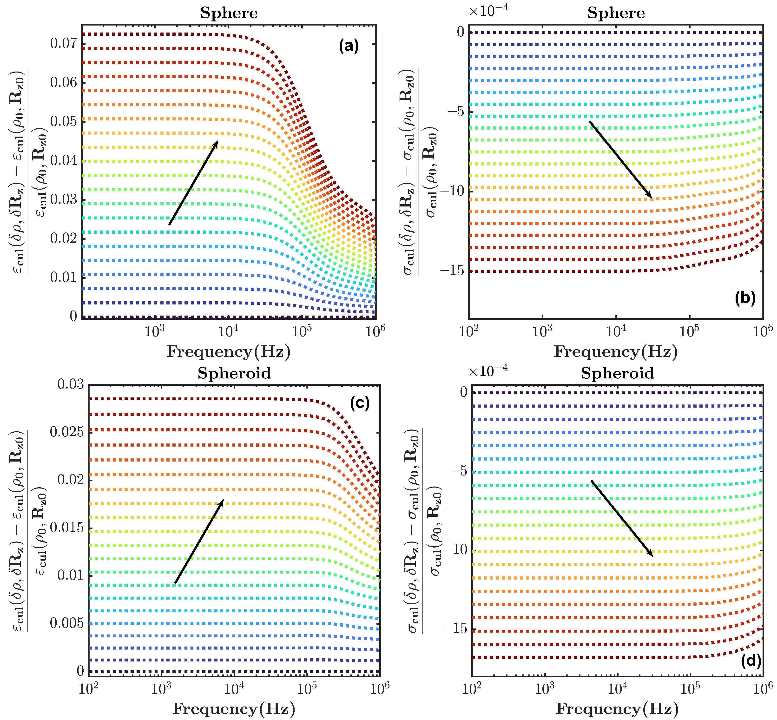
2. Theory
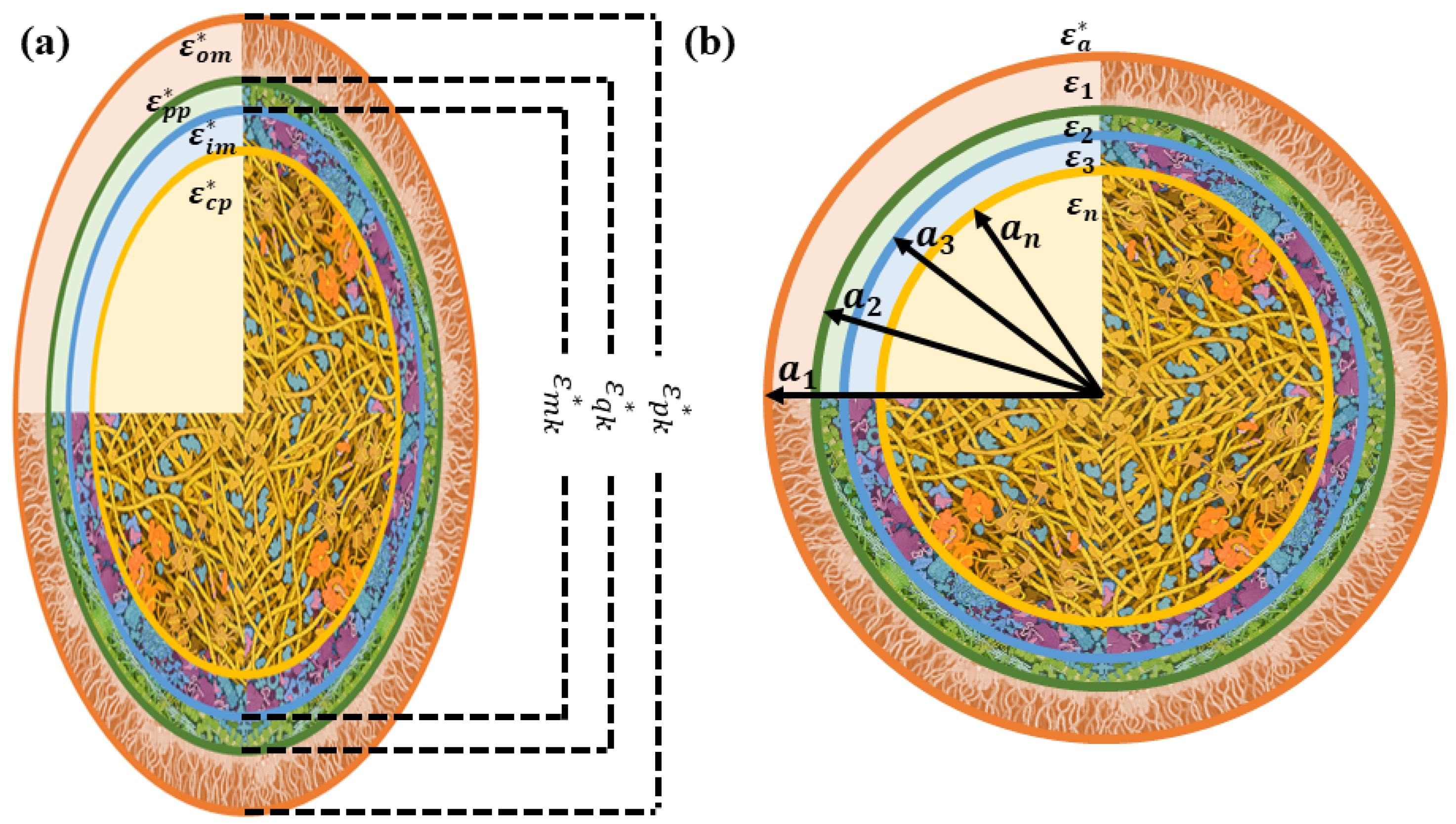
2.1. Modeling E. coli Bacterial Culture with Prolate Spheroidal Particles
2.2. Modeling E. coli Bacterial Culture with Spherical Particles
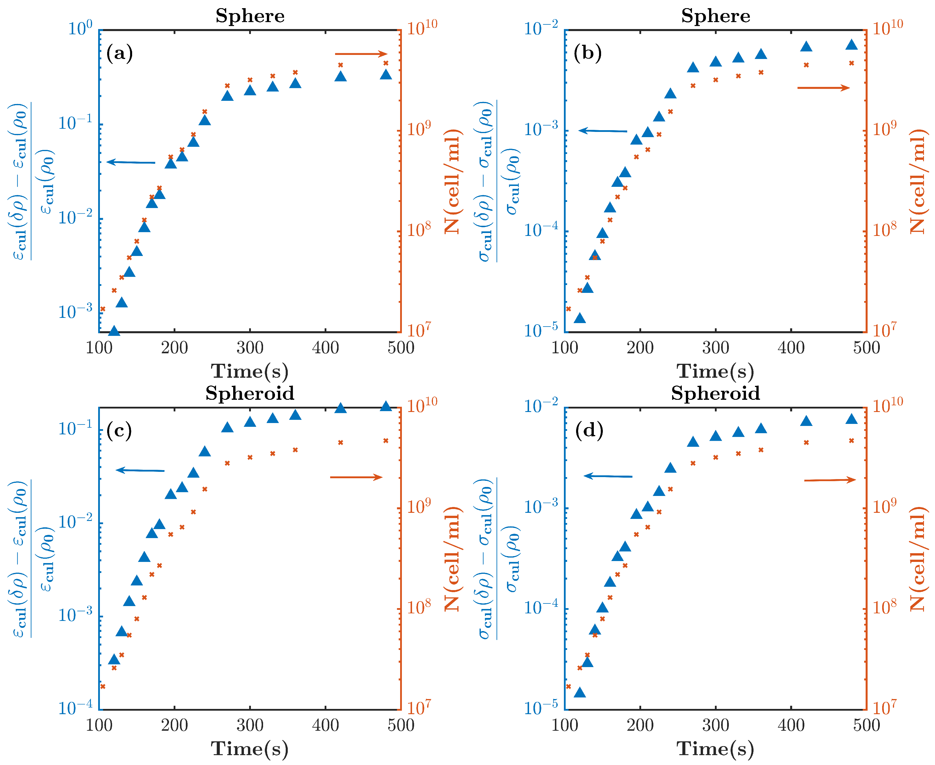
3. Mimicking the Functional Activity of Microorganisms: Duplication Process
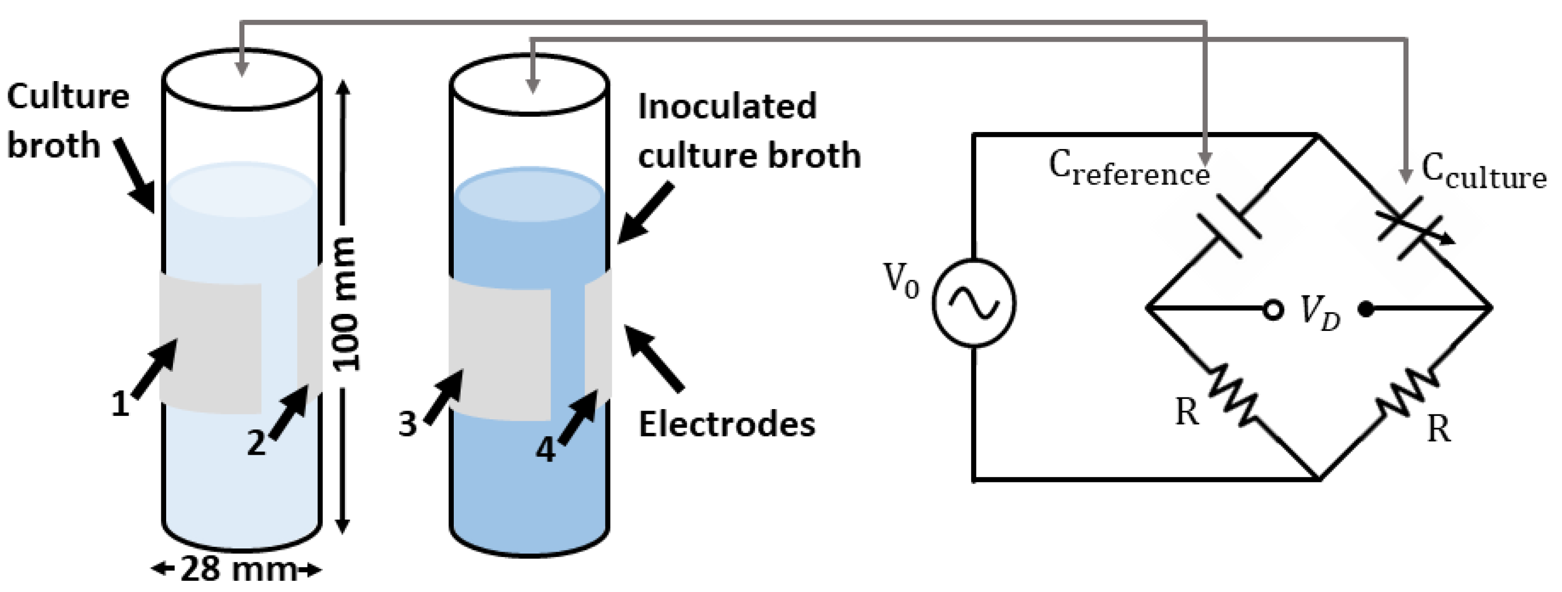
4. Experimental System and Procedures
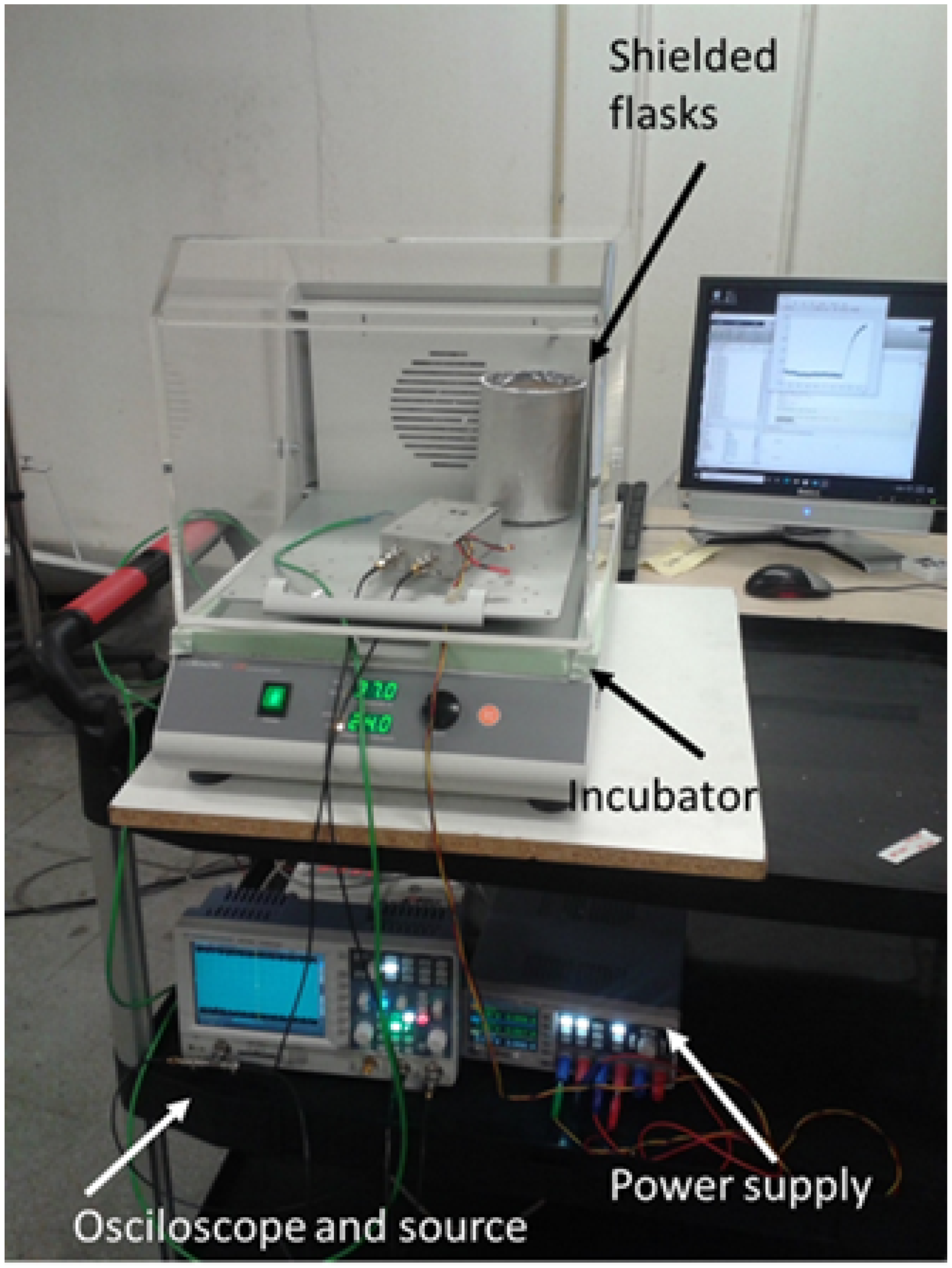
4.1. System Description
4.2. Cell Culture Growth Measurements
5. Discussion
6. Conclusions
Author Contributions
Funding
Institutional Review Board Statement
Informed Consent Statement
Data Availability Statement
Acknowledgments
Conflicts of Interest
Abbreviations
| OD | Optical diffusion |
| CMMR | Common-mode rejection ratio |
| GCM | Common-mode gain |
| GD | Differential gain |
| LB Broth | Lysogeny broth |
Appendix A
Appendix A.1. System Noise

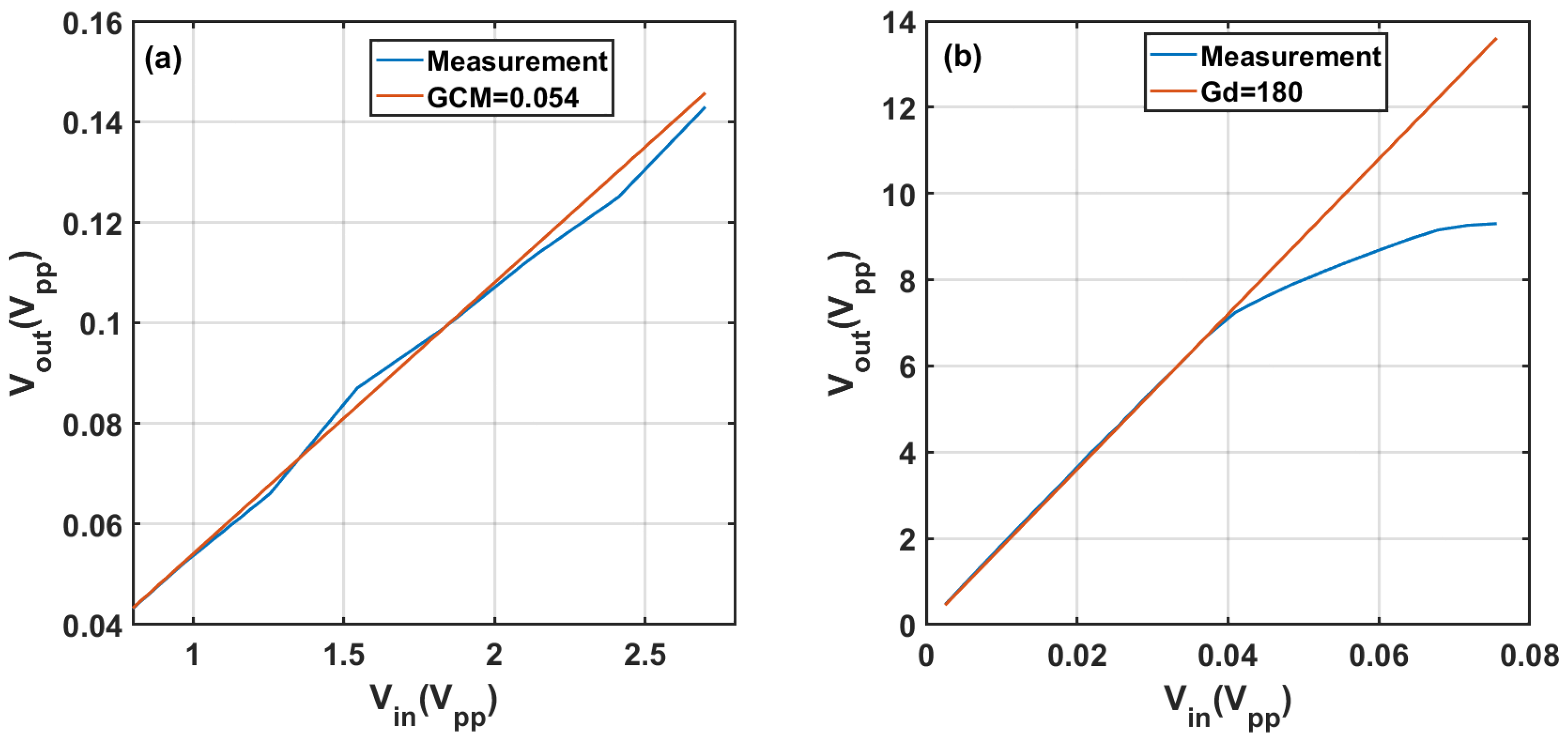
Appendix A.2. System Calibration


References
- Páez-Avilés, C.; Juanola-Feliu, E.; Punter-Villagrasa, J.; Del Moral Zamora, B.; Homs-Corbera, A.; Colomer-Farrarons, J.; Miribel-Català, P.L.; Samitier, J. Combined Dielectrophoresis and Impedance Systems for Bacteria Analysis in Microfluidic On-Chip Platforms. Sensors 2016, 16, 1514. [Google Scholar] [CrossRef] [PubMed] [Green Version]
- Hunt, R.W.; Zavalin, A.; Bhatnagar, A.; Chinnasamy, S.; Das, K.C. Electromagnetic biostimulation of living cultures for biotechnology, biofuel and bioenergy applications. Int. J. Mol. Sci. 2009, 10, 4515–4558. [Google Scholar] [CrossRef] [PubMed]
- Kirk, M.D.; Pires, S.M.; Black, R.E.; Caipo, M.; Crump, J.A.; Devleesschauwer, B.; Döpfer, D.; Fazil, A.; Fischer-Walker, C.L.; Hald, T.; et al. World Health Organization estimates of the global and regional disease burden of 22 foodborne bacterial, protozoal, and viral diseases, 2010: A data synthesis. PLoS Med. 2015, 12, e1001921. [Google Scholar]
- Heo, J.; Hua, S.Z. An overview of recent strategies in pathogen sensing. Sensors 2009, 9, 4483–4502. [Google Scholar] [CrossRef]
- Jofre, M.; Jofre, L.; Jofre-Roca, L. On the wireless microwave sensing of bacterial membrane potential in microfluidic-actuated platforms. Sensors 2021, 21, 3420. [Google Scholar] [CrossRef]
- Clausen, C.H.; Dimaki, M.; Bertelsen, C.V.; Skands, G.E.; Rodriguez-Trujillo, R.; Thomsen, J.D.; Svendsen, W.E. Bacteria detection and differentiation using impedance flow cytometry. Sensors 2018, 18, 3496. [Google Scholar] [CrossRef] [Green Version]
- Kong, T.F.; Shen, X.; Marcos; Yang, C.; Ibrahim, I.H. Dielectrophoretic trapping and impedance detection of Escherichia coli, Vibrio cholera, and Enterococci bacteria. Biomicrofluidics 2020, 14, 054105. [Google Scholar] [CrossRef]
- Romanenko, S.; Begley, R.; Harvey, A.R.; Hool, L.; Wallace, V.P. The interaction between electromagnetic fields at megahertz, gigahertz and terahertz frequencies with cells, tissues and organisms: Risks and potential. J. R. Soc. Interface 2017, 14, 20170585. [Google Scholar] [CrossRef] [Green Version]
- Bean, B.P. The action potential in mammalian central neurons. Nat. Rev. Neurosci. 2007, 8, 451–465. [Google Scholar] [CrossRef]
- Lobikin, M.; Chernet, B.; Lobo, D.; Levin, M. Resting potential, oncogene-induced tumorigenesis, and metastasis: The bioelectric basis of cancer in vivo. Phys. Biol. 2012, 9, 065002. [Google Scholar] [CrossRef] [Green Version]
- Ragab, M.A.; El-Kimary, E.I. Recent advances and applications of microfluidic capillary electrophoresis: A comprehensive review (2017–Mid 2019). Crit. Rev. Anal. Chem. 2021, 51, 709–741. [Google Scholar] [CrossRef] [PubMed]
- Sanchis, A.; Brown, A.; Sancho, M.; Martinez, G.; Sebastian, J.; Munoz, S.; Miranda, J. Dielectric characterization of bacterial cells using dielectrophoresis. BLCTDO 2007, 28, 393–401. [Google Scholar] [CrossRef] [PubMed]
- Asami, K. Characterization of heterogeneous systems by dielectric spectroscopy. Prog. Polym. Sci. 2002, 27, 1617–1659. [Google Scholar] [CrossRef]
- Prodan, C.; Mayo, F.; Claycomb, J.; Miller, J., Jr.; Benedik, M. Low-frequency, low-field dielectric spectroscopy of living cell suspensions. J. Appl. Phys. 2004, 95, 3754–3756. [Google Scholar] [CrossRef]
- Bai, W.; Zhao, K.; Asami, K. Dielectric properties of E. coli cell as simulated by the three-shell spheroidal model. Biophys. Chem. 2006, 122, 136–142. [Google Scholar] [CrossRef]
- Zarrinkhat, F.; Garrido, A.; Jofre, L.; Romeu, J.; Rius, J. Electromagnetic Monitoring of Biological Microorganisms. In Proceedings of the 13th European Conference on Antennas and Propagation, Krakow, Poland, 31 March–5 April 2019; pp. 1–5. [Google Scholar]
- Mangini, F.; Tedeschi, N.; Frezza, F.; Sihvola, A. Homogenization of a multilayer sphere as a radial uniaxial sphere: Features and limits. J. Electromagn. Waves Appl. 2014, 28, 916–931. [Google Scholar] [CrossRef]
- Asami, K.; Hanai, T.; Koizumi, N. Dielectric analysis of Escherichia coli suspensions in the light of the theory of interfacial polarization. Biophys. J. 1980, 31, 215–228. [Google Scholar] [CrossRef] [Green Version]
- Sihvola, A. Electromagnetic Mixing Formulas and Applications; Electromagnetic Waves, IET: London, UK, 1999. [Google Scholar]
- Yao, Z.; Davis, R.M.; Kishony, R.; Kahne, D.; Ruiz, N. Regulation of cell size in response to nutrient availability by fatty acid biosynthesis in Escherichia coli. Proc. Natl. Acad. Sci. USA 2012, 109, 15097–15098. [Google Scholar] [CrossRef] [Green Version]
- Asami, K. Characterization of biological cells by dielectric spectroscopy. J. Non. Cryst. Solids 2002, 305, 268–277. [Google Scholar] [CrossRef]
- Sezonov, G.; Joseleau-Petit, D.; d’Ari, R. Escherichia coli physiology in Luria-Bertani broth. J. Bacteriol. 2007, 189, 8746–8749. [Google Scholar] [CrossRef] [Green Version]
- Weiss, G. Wheatstone Bridge Sensitivity. IEEE Trans. Instrum. Meas. 1969, 18, 2–6. [Google Scholar] [CrossRef]
- Nagarajan, P.R.; George, B.; Kumar, V.J. A linearizing digitizer for wheatstone bridge based signal conditioning of resistive sensors. IEEE Sens. J. 2017, 17, 1696–1705. [Google Scholar] [CrossRef]
- Rogi, C.; Buffa, C.; De Milleri, N.; Gaggl, R.; Prefasi, E. A Fully-Differential Switched-Capacitor Dual-Slope Capacitance-To-Digital Converter (CDC) for a Capacitive Pressure Sensor. Sensors 2019, 19, 3673. [Google Scholar] [CrossRef] [Green Version]
- Malmberg, C.; Maryott, A. Dielectric constant of water from 0 to 100 C. J. Res. Natl. Inst. Stand. Technol. 1956, 56, 1–8. [Google Scholar] [CrossRef]


Publisher’s Note: MDPI stays neutral with regard to jurisdictional claims in published maps and institutional affiliations. |
© 2022 by the authors. Licensee MDPI, Basel, Switzerland. This article is an open access article distributed under the terms and conditions of the Creative Commons Attribution (CC BY) license (https://creativecommons.org/licenses/by/4.0/).
Share and Cite
Zarrinkhat, F.; Jofre-Roca, L.; Jofre, M.; Rius, J.M.; Romeu, J. Experimental Verification of Dielectric Models with a Capacitive Wheatstone Bridge Biosensor for Living Cells: E. coli. Sensors 2022, 22, 2441. https://doi.org/10.3390/s22072441
Zarrinkhat F, Jofre-Roca L, Jofre M, Rius JM, Romeu J. Experimental Verification of Dielectric Models with a Capacitive Wheatstone Bridge Biosensor for Living Cells: E. coli. Sensors. 2022; 22(7):2441. https://doi.org/10.3390/s22072441
Chicago/Turabian StyleZarrinkhat, Faezeh, Luís Jofre-Roca, Marc Jofre, Juan M. Rius, and Jordi Romeu. 2022. "Experimental Verification of Dielectric Models with a Capacitive Wheatstone Bridge Biosensor for Living Cells: E. coli" Sensors 22, no. 7: 2441. https://doi.org/10.3390/s22072441
APA StyleZarrinkhat, F., Jofre-Roca, L., Jofre, M., Rius, J. M., & Romeu, J. (2022). Experimental Verification of Dielectric Models with a Capacitive Wheatstone Bridge Biosensor for Living Cells: E. coli. Sensors, 22(7), 2441. https://doi.org/10.3390/s22072441