
Spatial Attention Frustum: A 3D Object Detection Method Focusing on Occluded Objects


Abstract
:1. Introduction
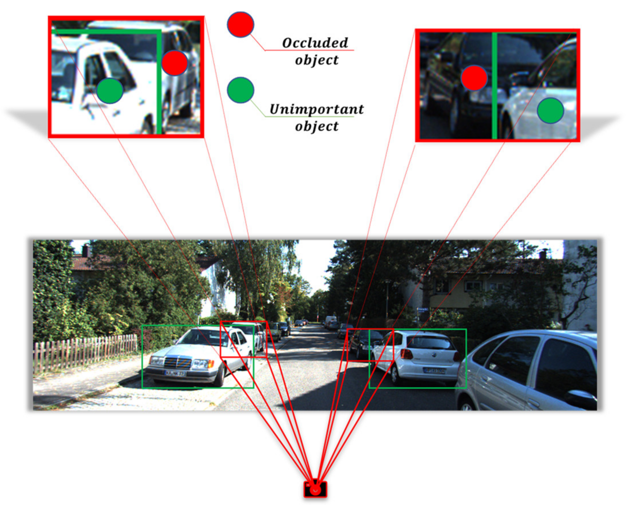
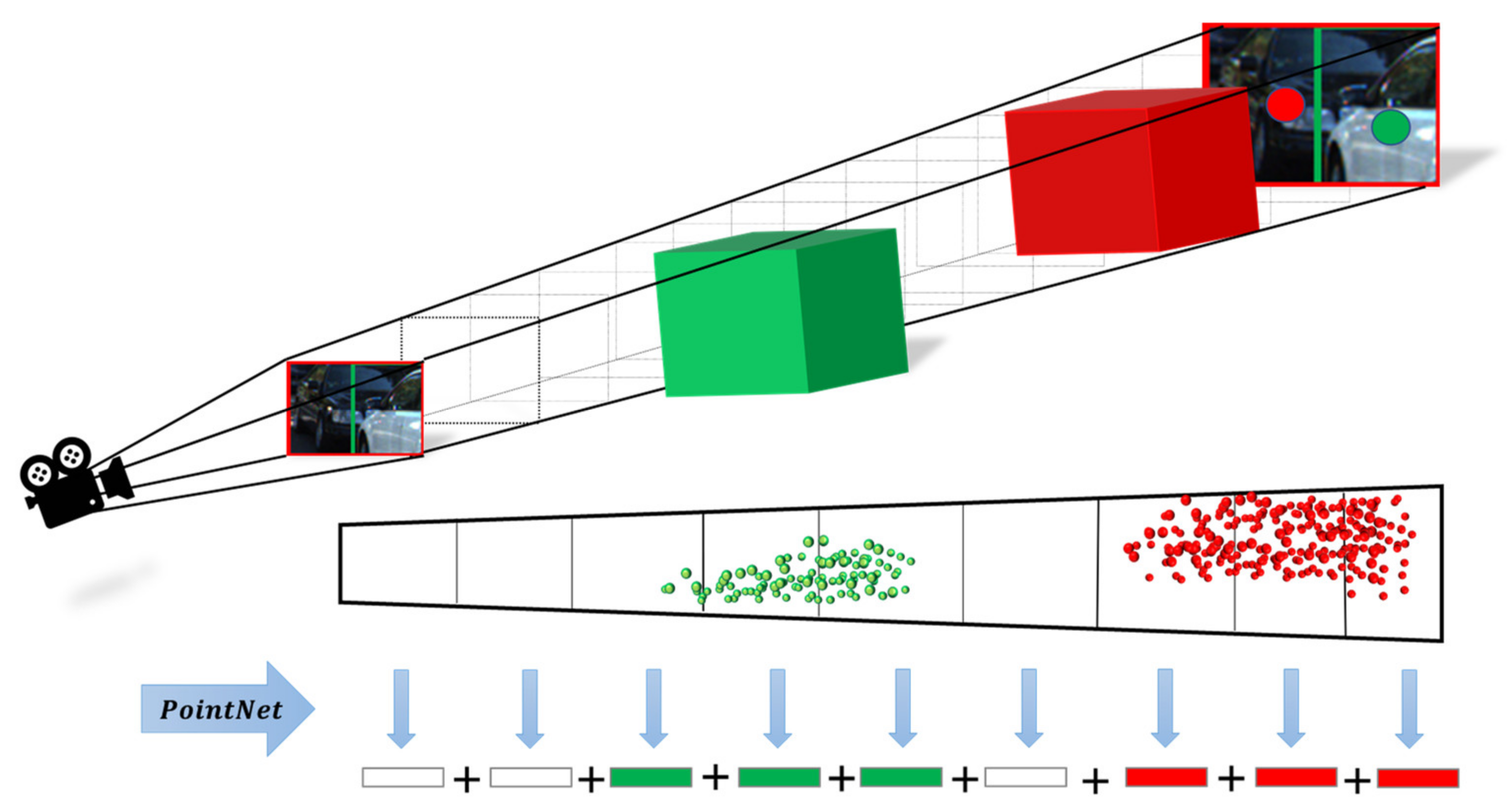
- We proposed the SAF, which simulates the human visual attention mechanism to position occluded objects in autonomous driving scenes accurately. The SAF can adaptively suppress unimportant features and allocate valuable computational resources to the occluded objects in the frustum so that the features of the occluded objects can be more effectively represented in the limited feature space.
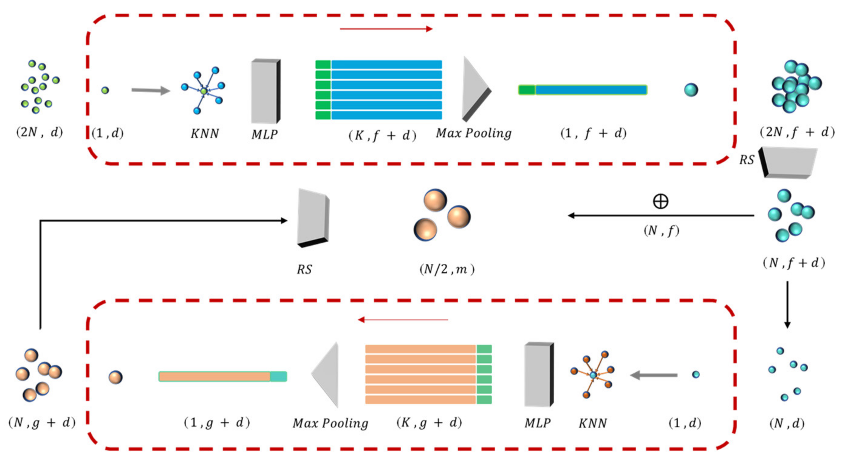
- Considering that the occluded objects usually have only the visible part of the point cloud, we proposed a point cloud local feature aggregation module to enhance the model’s ability to infer the whole from the local structure. The local feature aggregation module integrates more neighbourhood features, giving each point a larger perceptual field and allowing the model to learn more complex local features.
- We propose a joint anchor box PL function to obtain a more accurate boundary box prediction method by utilizing the projection constraint relationship between the 2D and 3D boxes. The experiment indicates that the joint anchor box PL function helps to improve the overall performance of the model.
- In the process of 3D object detection, our one-stage method can match the performance of the two-stage method without using refine stage, which makes our model more suitable for the autonomous driving scene in terms of real-time detection and the number of parameters.
2. Related Works
2.1. Image-Based 3D Object Detection Methods
2.2. LiDAR-Based 3D Object Detection Methods
2.3. Multi-Sensor-Based 3D Object Detection Methods
3. Materials and Methods
3.1. Spatial Attention Frustum (SAF) Module
SAF Segmentation Method
3.2. Local Feature Aggregation (LFA) Module
3.3. Feature Extractor and Fully Convolutional Network (FCN)
3.4. Projection Loss Function
4. Experiments
4.1. Dataset
4.2. Implementation Details
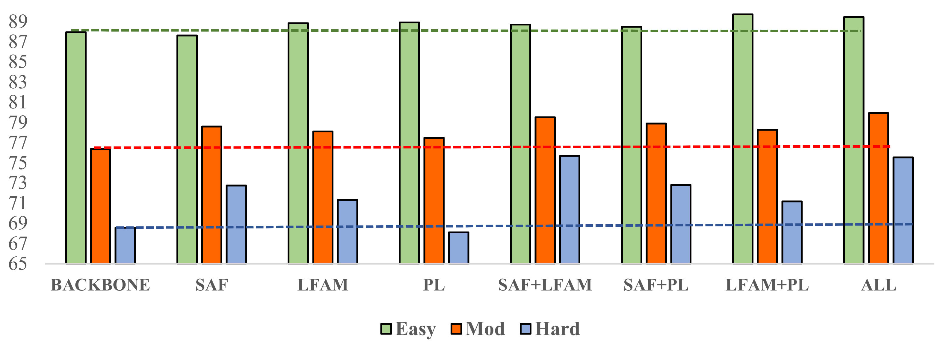
4.3. Ablation Study
4.3.1. Effects of the SAF Module
4.3.2. Effects of the LFA Module
4.3.3. Effects of the PL Loss Function
4.3.4. Effects of Feature Extractor
4.4. Qualitative Results
5. Discussion
6. Conclusions
Author Contributions
Funding
Institutional Review Board Statement
Informed Consent Statement
Data Availability Statement
Conflicts of Interest
References
- Gao, Q.; Shen, X. ThickSeg: Efficient semantic segmentation of large-scale 3D point clouds using multi-layer projection. Image Vis. Comput. 2021, 108, 104161. [Google Scholar] [CrossRef]
- Qin, P.; Zhang, C.; Dang, M. GVnet: Gaussian model with voxel-based 3D detection network for autonomous driving. Neural Comput. Appl. 2021, 5, 1–9. [Google Scholar] [CrossRef]
- Li, D.; Deng, L.; Cai, Z. Design of traffic object recognition system based on machine learning. Neural Comput. Appl. 2021, 33, 8143–8156. [Google Scholar] [CrossRef]
- Liang, W.; Xu, P.; Guo, L.; Bai, H.; Zhou, Y.; Chen, F. A survey of 3D object detection. Multimed. Tools Appl. 2021, 80, 29617–29641. [Google Scholar] [CrossRef]
- Yang, B.Y.; Du, X.P.; Fang, Y.Q.; Li, P.Y.; Wang, Y. Review of rigid object pose estimation from a single image. J. Image Graph. 2021, 26, 334–354. [Google Scholar]
- Zamanakos, G.; Tsochatzidis, L.; Amanatiadis, A.; Pratikakis, I. A comprehensive survey of LIDAR-based 3D object detection methods with deep learning for autonomous driving. Comput. Graph. 2021, 99, 153–181. [Google Scholar] [CrossRef]
- Ku, J.; Mozifian, M.; Lee, J.; Harakeh, A.; Waslander, S.L. Joint 3d proposal generation and object detection from view aggregation. In Proceedings of the IEEE/RSJ International Conference on Intelligent Robots and Systems (IROS), Madrid, Spain, 1–5 October 2018; pp. 1–8. [Google Scholar]
- Hao, W.; Wang, Y. Structure-based object detection from scene point clouds. Neurocomputing 2016, 191, 148–160. [Google Scholar] [CrossRef]
- Ye, Y.; Chen, H.; Zhang, C.; Hao, X.; Zhang, Z. SARPNET: Shape attention regional proposal network for liDAR-based 3D object detection. Neurocomputing 2020, 379, 53–63. [Google Scholar] [CrossRef]
- Chen, X.; Ma, H.; Wan, J.; Li, B.; Xia, T. Multi-view 3D Object Detection Network for Autonomous Driving. In Proceedings of the 2017 IEEE Conference on Computer Vision and Pattern Recognition (CVPR), Vancouver, BC, Canada, 24–28 September 2017; pp. 6526–6534. [Google Scholar]
- Qi, C.R.; Liu, W.; Wu, C.; Su, H.; Guibas, L.J. Frustum pointnets for 3D object detection from rgb-d data. In Proceedings of the IEEE Conference on Computer Vision and Pattern Recognition, Salt Lake City, UT, USA, 18–22 June 2018; pp. 918–927. [Google Scholar]
- Wang, Z.; Jia, K. Frustum convnet: Sliding frustums to aggregate local point-wise features for amodal 3D object detection. In Proceedings of the IEEE/RSJ International Conference on Intelligent Robots and Systems (IROS), Macau, China, 3–8 November 2019; pp. 1742–1749. [Google Scholar]
- Chen, X.; Kundu, K.; Zhang, Z.; Ma, H.; Fidler, S.; Urtasun, R. Monocular 3d object detection for autonomous driving. In Proceedings of the IEEE Conference on Computer Vision and Pattern Recognition, Las Vegas, NV, USA, 27–30 June 2016; pp. 2147–2156. [Google Scholar]
- Zhang, J.; Su, Q.; Wang, C.; Gu, H. Monocular 3D vehicle detection with multi-instance depth and geometry reasoning for autonomous driving. Neurocomputing 2020, 403, 182–192. [Google Scholar] [CrossRef]
- Brazil, G.; Liu, X. M3d-rpn: Monocular 3d region proposal network for object detection. In Proceedings of the IEEE/CVF International Conference on Computer Vision, Seoul, Korea, 27 October–2 November 2019; pp. 9287–9296. [Google Scholar]
- Weng, X.; Kitani, K. Monocular 3D object detection with pseudo-lidar point cloud. In Proceedings of the IEEE/CVF International Conference on Computer Vision Workshops, Seoul, Korea, 27–28 October 2019; pp. 857–866. [Google Scholar]
- Wang, X.; Yin, W.; Kong, T.; Jiang, Y.; Li, L.; Shen, C. Task-aware monocular depth estimation for 3D object detection. In Proceedings of the AAAI Conference on Artificial Intelligence, New York, NY, USA, 7–12 February 2020; Volume 34, pp. 12257–12264. [Google Scholar]
- Dewi, C.; Chen, R.C.; Liu, Y.T.; Jiang, X.; Hartomo, K.D. Yolo V4 for Advanced Traffic Sign Recognition with Synthetic Training Data Generated by Various GAN. IEEE Access 2021, 9, 97228–97242. [Google Scholar] [CrossRef]
- Zhou, Y.; Tuzel, O. VoxelNet: End-to-End Learning for Point Cloud Based 3D Object Detection. In Proceedings of the IEEE/CVF Conference on Computer Vision and Pattern Recognition, Salt Lake City, UT, USA, 18–23 June 2018; pp. 4490–4499. [Google Scholar]
- Yan, Y.; Mao, Y.; Li, B. SECOND: Sparsely Embedded Convolutional Detection. Sensors 2018, 18, 3337. [Google Scholar] [CrossRef] [PubMed] [Green Version]
- Lang, A.H.; Vora, S.; Caesar, H.; Zhou, L.; Yang, J.; Beijbom, O. Pointpillars: Fast encoders for object detection from point clouds. In Proceedings of the IEEE/CVF Conference on Computer Vision and Pattern Recognition, Long Beach, CA, USA, 15–20 June 2019; pp. 12697–12705. [Google Scholar]
- Shi, S.; Wang, X.; Li, H. Pointrcnn: 3D object proposal generation and detection from point cloud. In Proceedings of the IEEE/CVF Conference on Computer Vision and Pattern Recognition, Long Beach, CA, USA, 15–20 June 2019; pp. 770–779. [Google Scholar]
- Shi, S.; Wang, Z.; Shi, J.; Wang, X.; Li, H. From Points to Parts: 3D Object Detection from Point Cloud with Part-Aware and Part-Aggregation Network. IEEE Trans. Pattern Anal. Mach. Intell. 2020, 43, 1. [Google Scholar] [CrossRef] [PubMed] [Green Version]
- Ye, M.; Xu, S.; Cao, T. Hvnet: Hybrid voxel network for lidar based 3D object detection. In Proceedings of the IEEE/CVF Conference on Computer Vision and Pattern Recognition, Online, 14–19 June 2020; pp. 1631–1640. [Google Scholar]
- Wang, J.; Lan, S.; Gao, M.; Davis, L.S. Infofocus. In 3D Object Detection for Autonomous Driving with Dynamic Information Modeling. Proceedings of the European Conference on Computer Vision, Glasgow, UK, 23–28 August 2020; Springer: Berlin, Germany, 2020; pp. 405–420. [Google Scholar]
- Meyer, G.P.; Laddha, A.; Kee, E.; Vallespi-Gonzalez, C.; Wellington, C.K. Lasernet: An efficient probabilistic 3D object detector for autonomous driving. In Proceedings of the IEEE/CVF Conference on Computer Vision and Pattern Recognition, Long Beach, CA, USA, 15–20 June 2019; pp. 12677–12686. [Google Scholar]
- Wang, Z.; Ding, S.; Li, Y.; Zhao, M.; Roychowdhury, S.; Wallin, A.; Sapiro, G.; Qiu, Q. Range adaptation for 3D object detection in lidar. In Proceedings of the IEEE/CVF International Conference on Computer Vision Workshops, Seoul, Korea, 27–28 October 2019; pp. 2320–2328. [Google Scholar]
- Xu, D.; Anguelov, D.; Jain, A. Pointfusion: Deep sensor fusion for 3D bounding box estimation. In Proceedings of the IEEE Conference on Computer Vision and Pattern Recognition, Salt Lake City, UT, USA, 18–23 June; pp. 244–253.
- Ding, Z.; Han, X.; Niethammer, M. VoteNet. In A Deep Learning Label Fusion Method for Multi-Atlas Segmentation. Proceedings of the International Conference on Medical Image Computing and Computer-Assisted Intervention, Shenzhen, China, 13–17 October 2019; Springer: Berlin, Germany; pp. 202–210.
- Qi, C.R.; Chen, X.; Litany, O.; Guibas, L.J. Imvotenet: Boosting 3D object detection in point clouds with image votes. In Proceedings of the IEEE/CVF Conference on Computer Vision and Pattern Recognition, Online, 14–19 June 2020; pp. 4404–4413. [Google Scholar]
- Zhu, M.; Ma, C.; Ji, P.; Yang, X. Cross-modality 3D object detection. In Proceedings of the IEEE/CVF Winter Conference on Applications of Computer Vision, Waikoloa, HI, USA, 5–9 January 2021; pp. 3772–3781. [Google Scholar]
- Vora, S.; Lang, A.H.; Helou, B.; Beijbom, O. Pointpainting: Sequential fusion for 3D object detection. In Proceedings of the IEEE/CVF Conference on Computer Vision and Pattern Recognition, Online, 14–19 June 2020; pp. 4604–4612. [Google Scholar]
- Hu, Q.; Yang, B.; Xie, L.; Rosa, S.; Guo, Y.; Wang, Z.; Trigoni, N.; Markham, A. Randla-net: Efficient semantic segmentation of large-scale point clouds. In Proceedings of the IEEE/CVF Conference on Computer Vision and Pattern Recognition, Online, 14–19 June 2020; pp. 11108–11117. [Google Scholar]
- Qi, C.R.; Su, H.; Mo, K.; Guibas, L.J. Pointnet: Deep learning on point sets for 3D classification and segmentation. In Proceedings of the IEEE Conference on Computer Vision and Pattern Recognition, Honolulu, HI, USA, 21–26 July 2017; pp. 652–660. [Google Scholar]
- Lin, T.-Y.; Goyal, P.; Girshick, R.; He, K.; Dollár, P. Focal loss for dense object detection. In Proceedings of the IEEE International Conference on Computer Vision, Venice, Italy, 22–29 October 2017; pp. 2980–2988. [Google Scholar]
- Geiger, A.; Lenz, P.; Urtasun, R. Are we ready for autonomous driving? The kitti vision benchmark suite. In Proceedings of the IEEE Conference on Computer Vision and Pattern Recognition, Providence, RI, USA, 16–21 June 2012; pp. 3354–3361. [Google Scholar]
- Qi, C.R.; Yi, L.; Su, H.; Guibas, L.J. Pointnet++: Deep hierarchical feature learning on point sets in a metric space. arXiv 2017, 02413, 1706. [Google Scholar]
- Liang, M.; Yang, B.; Wang, S.; Urtasun, R. Deep continuous fusion for multi-sensor 3D object detection. In Proceedings of the European Conference on Computer Vision (ECCV), Munich, Germany, 8–14 September 2018; pp. 641–656. [Google Scholar]
- Wen, L.; Jo, K.-H. Three-Attention Mechanisms for One-Stage 3-D Object Detection Based on LiDAR and Camera. IEEE Trans. Ind. Inform. 2021, 17, 6655–6663. [Google Scholar] [CrossRef]
- Wen, L.-H.; Jo, K.-H. Fast and Accurate 3D Object Detection for Lidar-Camera-Based Autonomous Vehicles Using One Shared Voxel-Based Backbone. IEEE Access 2021, 9, 22080–22089. [Google Scholar] [CrossRef]


| Scale | Num A | Num B |
|---|---|---|
| T | 1 | T-1 |
| T/2 | 1 | T/2-1 |
| T/4 | 1 | T/4-1 |
| T/8 | 1 | T/8-1 |
| Level | Min Bounding Box Height | Max Occlusion Level | Max Truncation |
|---|---|---|---|
| Easy | 40 Px | Fully visible | 15% |
| Moderate | 25 Px | Partly occluded | 30% |
| Hard | 25 Px | Difficult to see | 50% |
| Backbone | SAF | LFA | PL | Easy | Mod | Hard |
|---|---|---|---|---|---|---|
| Yes | 87.95 | 76.37 | 68.56 | |||
| Yes | Yes | 87.62 (−0.33) | 78.59 (+2.22) | 72.74 (+4.18) | ||
| Yes | Yes | 88.84 (+0.89) | 78.11 (+1.74) | 71.33 (+2.77) | ||
| Yes | Yes | 88.91 (+0.96) | 77.48 (+1.11) | 68.09 (−0.47) | ||
| Yes | Yes | Yes | 88.71 (+0.76) | 79.52(+3.15) | 75.69 (+7.13) | |
| Yes | Yes | Yes | 88.48 (+0.53) | 78.89 (+2.52) | 72.81 (+4.25) | |
| Yes | Yes | Yes | 89.72 (+1.77) | 78.27 (+1.90) | 71.17 (+2.61) | |
| Yes | Yes | Yes | Yes | 89.46 (+1.51) | 79.91 (+3.54) | 75.53 (+6.97) |
| Method | Stage | Number of Parameters | Runtime (s) | AP3D (Cars) | APBEV (Cars) | ||||
|---|---|---|---|---|---|---|---|---|---|
| Easy | Mod | Hard | Easy | Mod | Hard | ||||
| F-pointnet | Two | - | - | 83.76 | 70.92 | 63.65 | 88.16 | 84.02 | 76.44 |
| Backbone + Refine | Two | 6,633,554 | 0.49 | 88.98 | 78.66 | 72.23 | 90.08 | 88.84 | 80.10 |
| Backbone | One | 3,316,777 | 0.26 | 87.95 | 76.37 | 68.56 | 89.88 | 87.48 | 78.99 |
| Ours | One | 3,724,013 | 0.29 | 89.46 | 79.91 | 75.53 | 91.27 | 89.63 | 85.75 |
| Method | Stage | Number of Parameters | Runtime (s) | AP3D (Pedestrians) | APBEV (Pedestrians) | ||||
|---|---|---|---|---|---|---|---|---|---|
| Easy | Mod | Hard | Easy | Mod | Hard | ||||
| F-pointnet | Two | - | - | 70.00 | 61.32 | 53.59 | 72.38 | 66.39 | 59.57 |
| Backbone + Refine | Two | 6,633,554 | 0.49 | 70.88 | 62.24 | 53.37 | 72.59 | 67.05 | 58.68 |
| Backbone | One | 3,316,777 | 0.26 | 68.47 | 60.63 | 50.80 | 70.31 | 66.14 | 56.09 |
| Ours | One | 3,724,013 | 0.29 | 70.61 | 61.84 | 53.93 | 72.24 | 66.58 | 59.11 |
| Method | Stage | Number of Parameters | Runtime (s) | AP3D (Cyclists) | APBEV (Cyclists) | ||||
|---|---|---|---|---|---|---|---|---|---|
| Easy | Mod | Hard | Easy | Mod | Hard | ||||
| F-pointnet | Two | - | - | 77.15 | 56.49 | 53.37 | 81.82 | 60.03 | 56.32 |
| Backbone + Refine | Two | 6,633,554 | 0.49 | 81.69 | 69.55 | 59.87 | 83.28 | 70.10 | 61.79 |
| Backbone | One | 3,316,777 | 0.26 | 75.88 | 64.63 | 55.74 | 80.37 | 63.24 | 57.52 |
| Ours | One | 3,724,013 | 0.29 | 77.24 | 65.21 | 56.15 | 80.79 | 66.47 | 57.86 |
| Method | Modality | AP3D (Cars) | APBEV (Cars) | ||||
|---|---|---|---|---|---|---|---|
| Easy | Mod | Hard | Easy | Mod | Hard | ||
| VoxelNet [15] | LiDAR | 81.97 | 65.46 | 62.85 | 89.60 | 84.81 | 78.57 |
| SECOND [16] | LiDAR | 87.43 | 76.48 | 69.10 | 89.96 | 87.07 | 79.66 |
| PointRCNN [18] | LiDAR | 88.88 | 78.63 | 77.38 | 90.21 | 87.89 | 85.51 |
| ContFuse [34] | LiDAR + RGB | 86.32 | 73.25 | 67.81 | 95.44 | 87.34 | 82.43 |
| AVODFPN [4] | LiDAR + RGB | 84.41 | 74.44 | 68.65 | - | - | - |
| F-pointnet [8] | LiDAR + RGB | 83.76 | 70.92 | 63.65 | 88.16 | 84.92 | 76.44 |
| FconvNet [9] | LiDAR + RGB | 89.02 | 78.80 | 77.09 | 90.23 | 88.79 | 86.84 |
| Ours | LiDAR + RGB | 89.46 | 79.91 | 75.53 | 91.27 | 89.63 | 85.75 |
Publisher’s Note: MDPI stays neutral with regard to jurisdictional claims in published maps and institutional affiliations. |
© 2022 by the authors. Licensee MDPI, Basel, Switzerland. This article is an open access article distributed under the terms and conditions of the Creative Commons Attribution (CC BY) license (https://creativecommons.org/licenses/by/4.0/).
Share and Cite
He, X.; Zhang, X.; Wang, Y.; Ji, H.; Duan, X.; Guo, F. Spatial Attention Frustum: A 3D Object Detection Method Focusing on Occluded Objects. Sensors 2022, 22, 2366. https://doi.org/10.3390/s22062366
He X, Zhang X, Wang Y, Ji H, Duan X, Guo F. Spatial Attention Frustum: A 3D Object Detection Method Focusing on Occluded Objects. Sensors. 2022; 22(6):2366. https://doi.org/10.3390/s22062366
Chicago/Turabian StyleHe, Xinglei, Xiaohan Zhang, Yichun Wang, Hongzeng Ji, Xiuhui Duan, and Fen Guo. 2022. "Spatial Attention Frustum: A 3D Object Detection Method Focusing on Occluded Objects" Sensors 22, no. 6: 2366. https://doi.org/10.3390/s22062366
APA StyleHe, X., Zhang, X., Wang, Y., Ji, H., Duan, X., & Guo, F. (2022). Spatial Attention Frustum: A 3D Object Detection Method Focusing on Occluded Objects. Sensors, 22(6), 2366. https://doi.org/10.3390/s22062366