
Multi-Feature Single Target Robust Tracking Fused with Particle Filter


Abstract
:1. Introduction
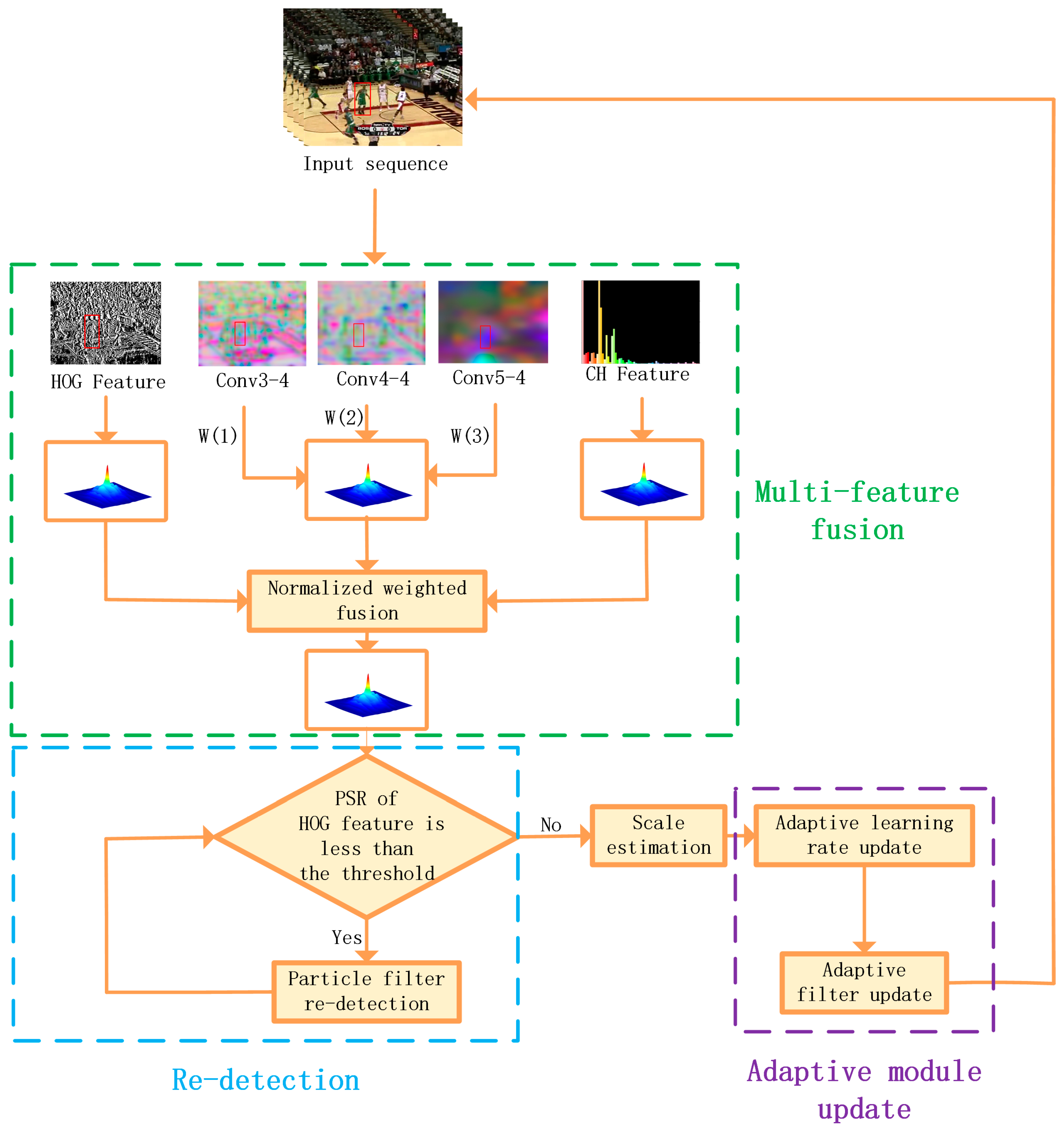
- First, the feature response matrix of three features, namely HOG features, CH features and depth features, is fused to train a more robust appearance model to improve the robustness of the algorithm in target tracking under complex environments such as severe target deformation, occlusion, fast motion, out-of-field, and similar colors;
- Second, we design a re-detection module incorporating particle filtering to address the problem of how to return to accurate tracking after the target tracking fails due to complex factors such as complete occlusion, deformation and blurring, so that the algorithm in this paper can maintain high robustness and efficiency when tracking for a long time;
- Third, in this paper, two parts, adaptive learning rate update and adaptive filter update, are performed in the adaptive model update phase to improve the robustness of the target model in this paper’s algorithm;
- Fourth, the proposed tracking algorithm is evaluated on the dataset OTB-2015, dataset OTB-2013 and dataset UAV123. and the experimental results show that the proposed algorithm exhibits more stable and accurate tracking performance in the case of severe target deformation, occlusion, fast motion, and out-of-field during tracking.
2. Related Work
2.1. Correlation Filtering
2.2. Tracking by Deep Neural Networks
3. The Proposed Method
3.1. Correlation Filtering Architecture
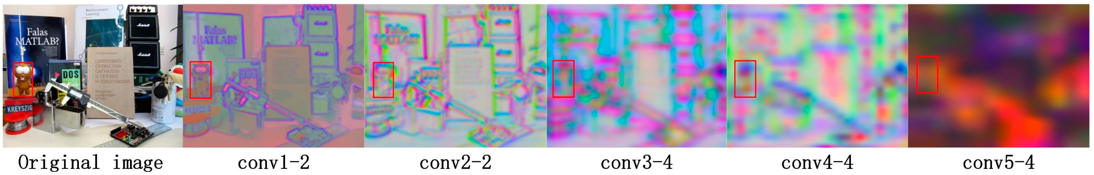
3.2. Multi-Feature Fusion
3.3. Particle Filtering Re-Detection
3.4. Adaptive Update
3.4.1. Adaptive Learning Rate Update
3.4.2. Adaptive Filter Update
| Algorithm 1: Multi-Feature Single-Target Robust Tracking Algorithm Fused with Particle Filter |
| Input: initial target position and other initialization parameters Output: estimated target location 1. Enter the first frame and initialize the target filter model; 2. for i = 2,3,…, until the last frame do 3. Determine the search window in the i-th frame; 4. Extract the HOG, CH and depth features and calculate the corresponding correlation response maps; 5. Feature fusion using (6); 6. Use (6) to calculate the score of the current target ; 7. if then 8. Particle filtering re-detection for the current frame target; 9. Use Equation (10) to calculate the confidence of the candidate; 10. Choose the best candidate ; 11. end if 12. Determine the optimal scale of the target and calculate the scale filter; 13. Use (11) to adaptively update the learning rate ; 14. Use (12) to calculate APCE value; 15. if APCE > 0.45 * APCE_Average and > 0.6 * Average then 16. Use (4) and (5) to update the filter; 17. end if 18. end for |
4. Implementation Details
5. Experiment Results and Analysis
5.1. Experiments on the OTB2015
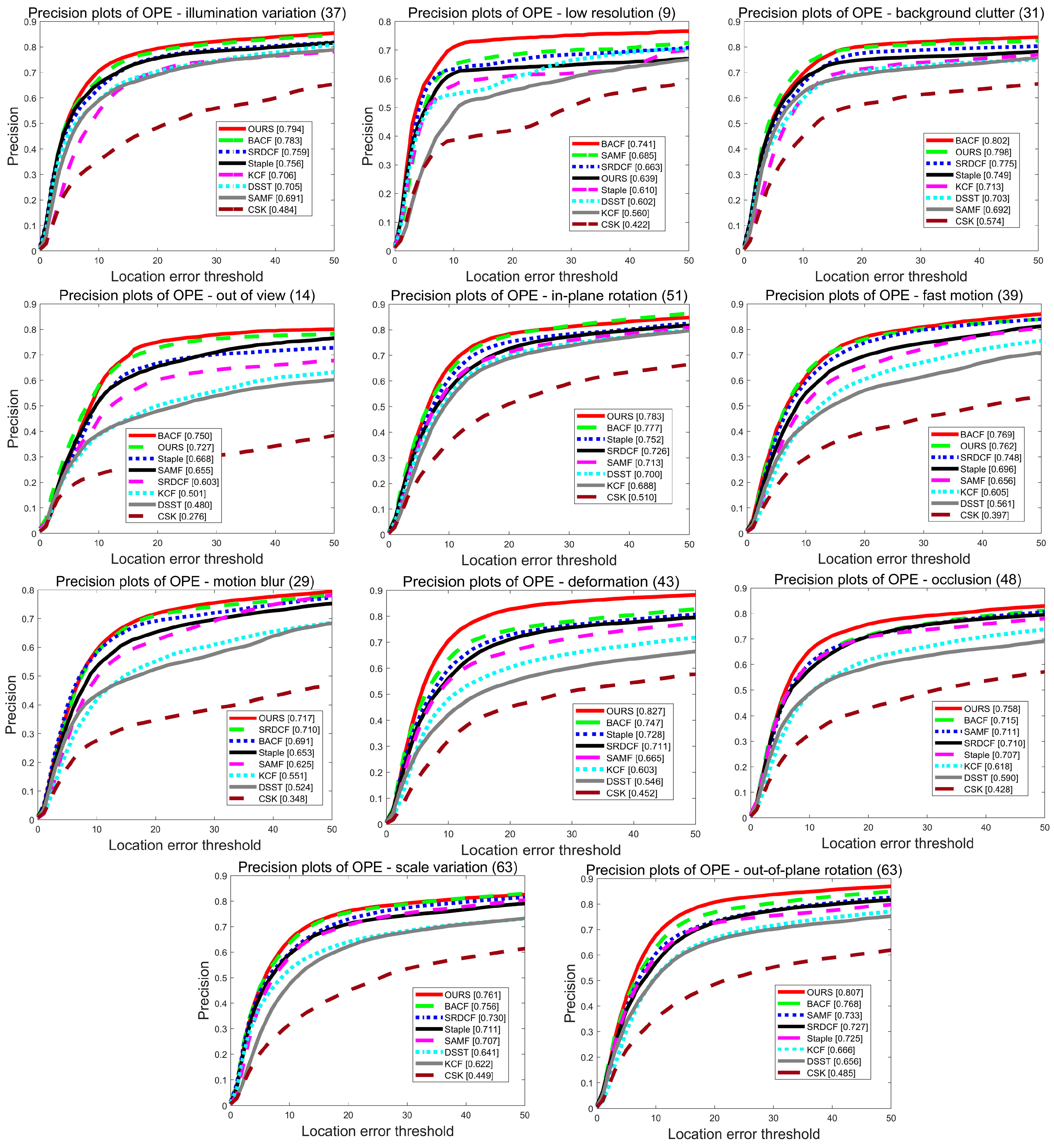
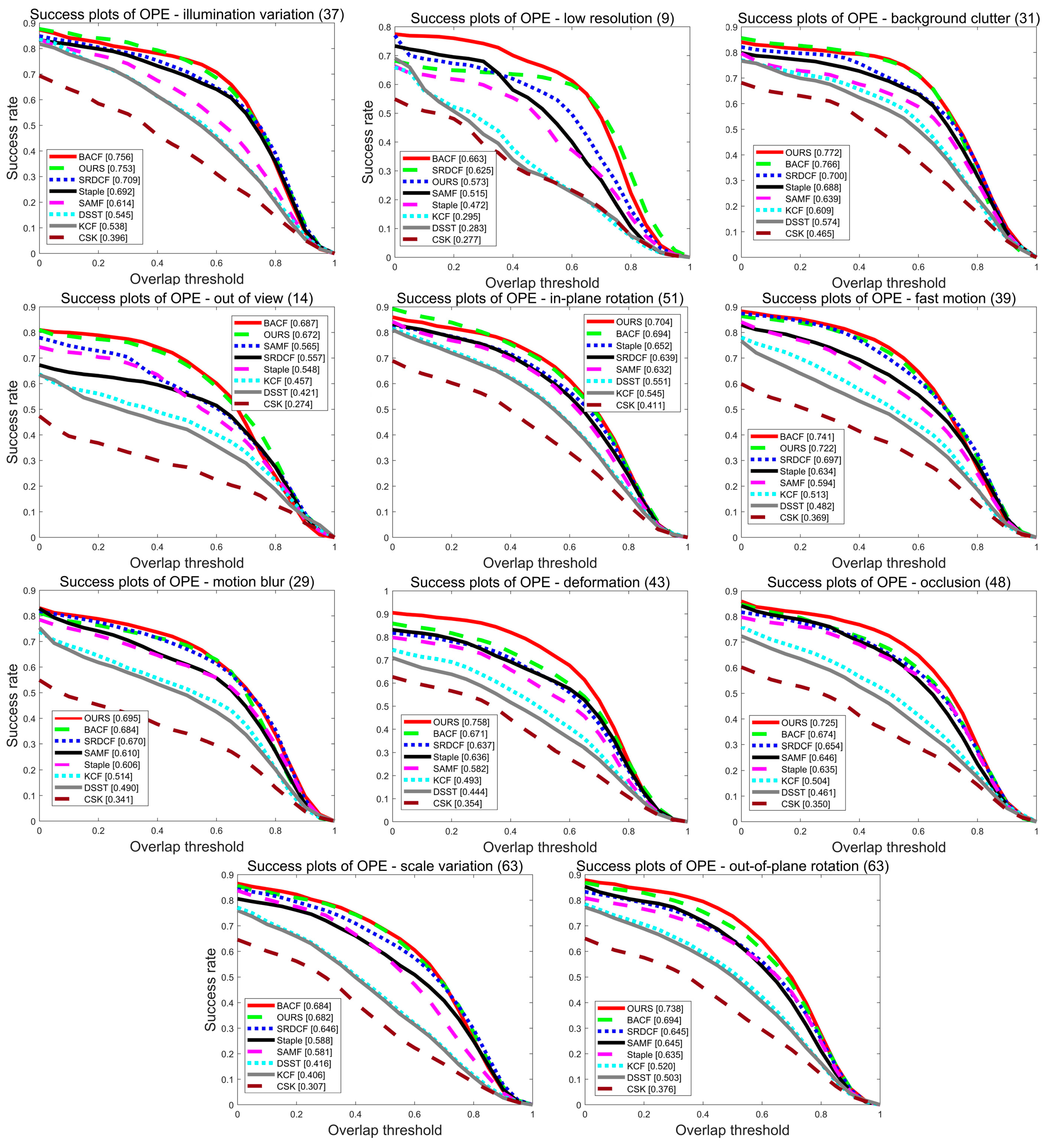
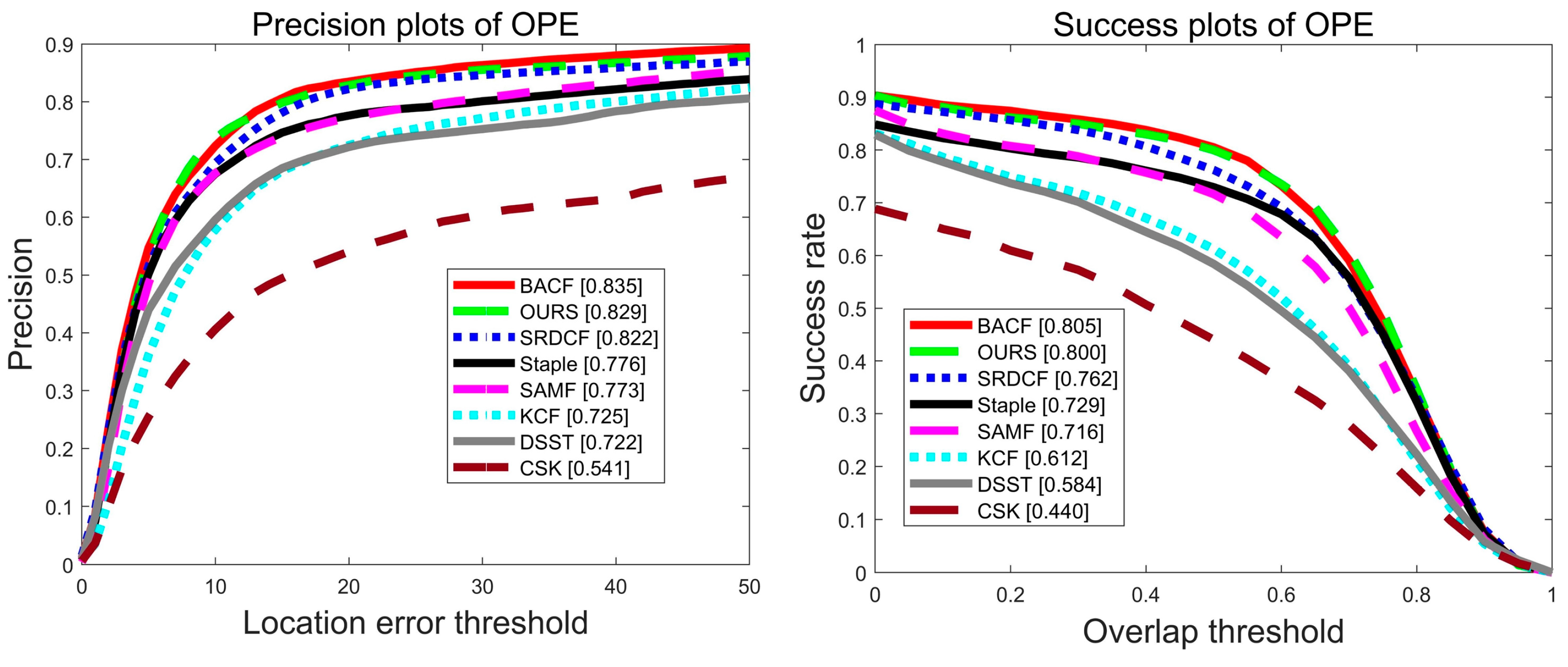
5.1.1. Quantitative Analysis
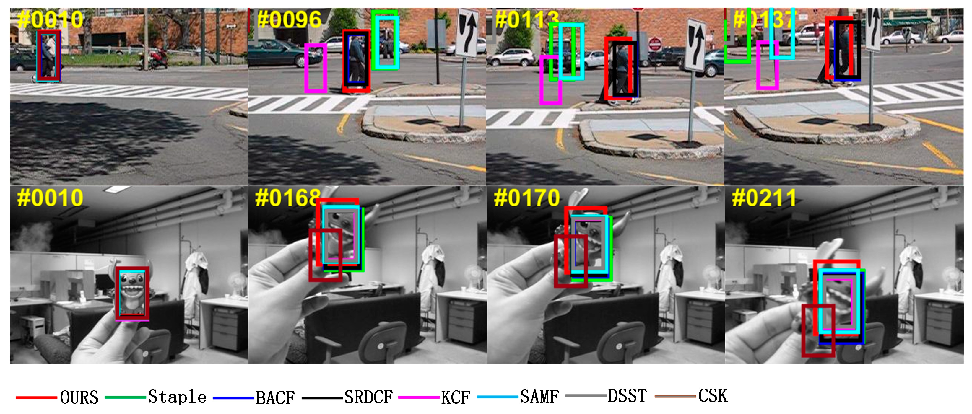
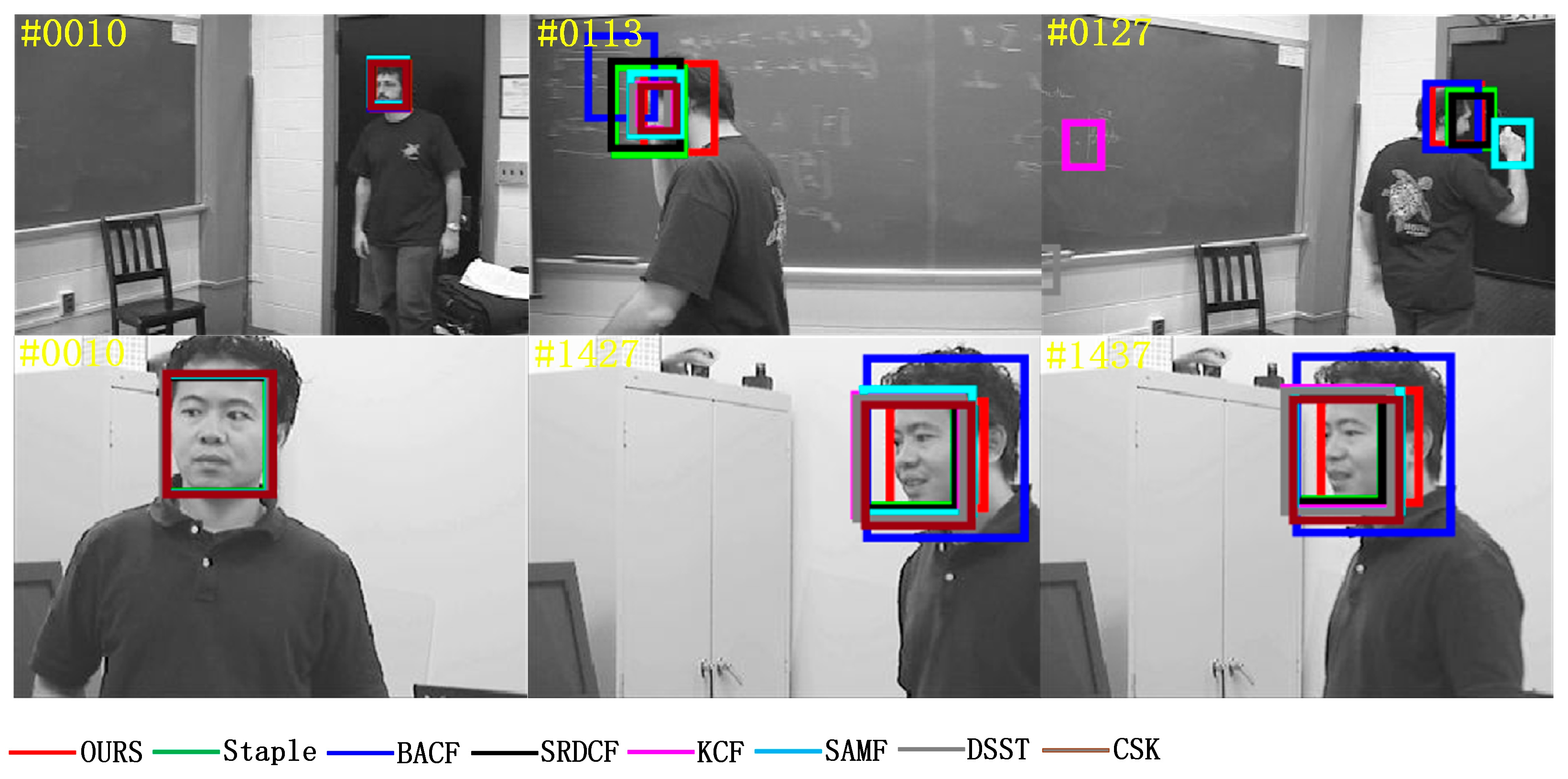
5.1.2. Qualitative Analysis
5.2. Experiments on the OTB2013
5.2.1. Quantitative Analysis
5.2.2. Ablation Experiment
5.3. Experiments on the UAV123
6. Conclusions
Author Contributions
Funding
Institutional Review Board Statement
Informed Consent Statement
Data Availability Statement
Conflicts of Interest
References
- Janai, J.; Güney, F.; Behl, A.; Geiger, A. Computer vision for autonomous vehicles: Problems, datasets and state of the art. In Foundations and Trends® in Computer Graphics and Vision; Now Publishers: Norwell, MA, USA; Delft, The Netherlands, 2020; Volume 12, pp. 1–308. [Google Scholar]
- Ruan, W.; Chen, J.; Wu, Y.; Wang, J.; Liang, C.; Hu, R.; Jiang, J. Multi-correlation filters with triangle-structure constraints for object tracking. IEEE Trans. Multimed. 2018, 21, 1122–1134. [Google Scholar] [CrossRef]
- Previtali, F.; Bloisi, D.D.; Iocchi, L. A distributed approach for real-time multi-camera multiple object tracking. Mach. Vis. Appl. 2017, 28, 421–430. [Google Scholar] [CrossRef]
- Rautaray, S.S.; Agrawal, A. Vision based hand gesture recognition for human computer interaction: A survey. Artif. Intell. Rev. 2015, 43, 1–54. [Google Scholar] [CrossRef]
- Liu, Y.; Jing, X.-Y.; Nie, J.; Gao, H.; Liu, J.; Jiang, G.-P. Context-aware three-dimensional mean-shift with occlusion handling for robust object tracking in RGB-D videos. IEEE Trans. Multimed. 2018, 21, 664–677. [Google Scholar] [CrossRef]
- Mueller, M.; Smith, N.; Ghanem, B. A benchmark and simulator for UAV tracking. In Computer Vision—ECCV 2016, Proceedings of the European Conference on Computer Vision, Amsterdam, The Netherlands, 11–14 October 2016; Springer: Cham, Switzerland, 2016; pp. 445–461. [Google Scholar]
- Wang, T.; Zhang, G.; Bhuiyan, M.Z.A.; Liu, A.; Jia, W.; Xie, M. A novel trust mechanism based on fog computing in sensor-cloud system. Future Gener. Comput. Syst. 2020, 109, 573–582. [Google Scholar] [CrossRef]
- Meng, L.; Yang, X. A survey of object tracking algorithms. Acta Autom. Sin. 2019, 45, 1244–1260. [Google Scholar]
- Li, P.; Wang, D.; Wang, L.; Lu, H. Deep visual tracking: Review and experimental comparison. Pattern Recognit. 2018, 76, 323–338. [Google Scholar] [CrossRef]
- Wang, X.; Wang, G.; Zhao, Z.; Zhang, Y.; Duan, B. An improved kernelized correlation filter algorithm for underwater target tracking. Appl. Sci. 2018, 8, 2154. [Google Scholar] [CrossRef] [Green Version]
- Zhao, Q.; Yang, Z.; Tao, H. Differential earth mover’s distance with its applications to visual tracking. IEEE Trans. Pattern Anal. Mach. Intell. 2008, 32, 274–287. [Google Scholar] [CrossRef] [Green Version]
- Dalal, N.; Triggs, B. Histograms of oriented gradients for human detection. In Proceedings of the 2005 IEEE Computer Society Conference on Computer Vision and Pattern Recognition (CVPR’05), San Diego, CA, USA, 20–25 June 2005; pp. 886–893. [Google Scholar]
- Van De Weijer, J.; Schmid, C.; Verbeek, J.; Larlus, D. Learning color names for real-world applications. IEEE Trans. Image Process. 2009, 18, 1512–1523. [Google Scholar] [CrossRef] [Green Version]
- Simonyan, K.; Zisserman, A. Very deep convolutional networks for large-scale image recognition. arXiv 2014, arXiv:1409.1556. [Google Scholar]
- Ma, C.; Huang, J.-B.; Yang, X.; Yang, M.-H. Robust visual tracking via hierarchical convolutional features. IEEE Trans. Pattern Anal. Mach. Intell. 2018, 41, 2709–2723. [Google Scholar] [CrossRef] [Green Version]
- Deng, J.; Dong, W.; Socher, R.; Li, L.-J.; Li, K.; Fei-Fei, L. Imagenet: A large-scale hierarchical image database. In Proceedings of the 2009 IEEE Conference on Computer Vision and Pattern Recognition, Miami, FL, USA, 20–25 June 2009; pp. 248–255. [Google Scholar]
- Bolme, D.S.; Beveridge, J.R.; Draper, B.A.; Lui, Y.M. Visual object tracking using adaptive correlation filters. In Proceedings of the 2010 IEEE Computer Society Conference on Computer Vision and Pattern Recognition, San Francisco, CA, USA, 13–18 June 2010; pp. 2544–2550. [Google Scholar]
- Henriques, J.F.; Caseiro, R.; Martins, P.; Batista, J. Exploiting the circulant structure of tracking-by-detection with kernels. In Computer Vision—ECCV 2012, Proceedings of the European Conference on Computer Vision, Florence, Italy, 7–13 October 2012; Springer: Berlin/Heidelberg, Germany, 2012; pp. 702–715. [Google Scholar]
- Voigtlaender, P.; Luiten, J.; Torr, P.H.; Leibe, B. Siam R-CNN: Visual tracking by re-detection. In Proceedings of the IEEE/CVF Conference on Computer Vision and Pattern Recognition, Seattle, WA, USA, 14–19 June 2020; pp. 6578–6588. [Google Scholar]
- Henriques, J.F.; Caseiro, R.; Martins, P.; Batista, J. High-speed tracking with kernelized correlation filters. IEEE Trans. Pattern Anal. Mach. Intell. 2014, 37, 583–596. [Google Scholar] [CrossRef] [Green Version]
- Danelljan, M.; Häger, G.; Khan, F.; Felsberg, M. Accurate scale estimation for robust visual tracking. In Proceedings of the British Machine Vision Conference, Nottingham, UK, 1–5 September 2014; BMVA Press: Durham, UK, 2014. [Google Scholar]
- Li, Y.; Zhu, J. A scale adaptive kernel correlation filter tracker with feature integration. In Computer Vision—ECCV 2014, Proceedings of the European Conference on Computer Vision, Zurich, Switzerland, 6–12 September 2014; Springer: Cham, Switzerland, 2014; pp. 254–265. [Google Scholar]
- Danelljan, M.; Hager, G.; Shahbaz Khan, F.; Felsberg, M. Learning spatially regularized correlation filters for visual tracking. In Proceedings of the IEEE International Conference on Computer Vision, Santiago, Chile, 7–13 December 2015; pp. 4310–4318. [Google Scholar]
- Kiani Galoogahi, H.; Sim, T.; Lucey, S. Correlation filters with limited boundaries. In Proceedings of the IEEE Conference on Computer Vision and Pattern Recognition, Boston, MA, USA, 7–12 June 2015; pp. 4630–4638. [Google Scholar]
- Ma, C.; Yang, X.; Zhang, C.; Yang, M.-H. Long-term correlation tracking. In Proceedings of the IEEE Conference on Computer Vision and Pattern Recognition, Boston, MA, USA, 7–12 June 2015; pp. 5388–5396. [Google Scholar]
- Bertinetto, L.; Valmadre, J.; Golodetz, S.; Miksik, O.; Torr, P.H. Staple: Complementary learners for real-time tracking. In Proceedings of the IEEE Conference on Computer Vision and Pattern Recognition, Las Vegas, NV, USA, 27–30 June 2016; pp. 1401–1409. [Google Scholar]
- Lukezic, A.; Vojir, T.; Cehovin Zajc, L.; Matas, J.; Kristan, M. Discriminative correlation filter with channel and spatial reliability. In Proceedings of the IEEE Conference on Computer Vision and Pattern Recognition, Honolulu, HI, USA, 21–26 July 2017; pp. 6309–6318. [Google Scholar]
- Kiani Galoogahi, H.; Fagg, A.; Lucey, S. Learning background-aware correlation filters for visual tracking. In Proceedings of the IEEE International Conference on Computer Vision, Venice, Italy, 22–29 October 2017; pp. 1135–1143. [Google Scholar]
- Mueller, M.; Smith, N.; Ghanem, B. Context-aware correlation filter tracking. In Proceedings of the IEEE Conference on Computer Vision and Pattern Recognition, Honolulu, HI, USA, 21–26 July 2017; pp. 1396–1404. [Google Scholar]
- Cao, Y.; Ji, H.; Zhang, W.; Xue, F. Learning spatio-temporal context via hierarchical features for visual tracking. Signal Process. Image Commun. 2018, 66, 50–65. [Google Scholar] [CrossRef]
- Fan, J.; Xu, W.; Wu, Y.; Gong, Y. Human tracking using convolutional neural networks. IEEE Trans. Neural Netw. 2010, 21, 1610–1623. [Google Scholar] [PubMed]
- Wang, N.; Yeung, D.Y. Learning a deep compact image representation for visual tracking. Adv. Neural Inf. Process. Syst. 2013, 26, 809–817. [Google Scholar]
- Wang, L.; Liu, T.; Wang, G.; Chan, K.L.; Yang, Q. Video tracking using learned hierarchical features. IEEE Trans. Image Process. 2015, 24, 1424–1435. [Google Scholar] [CrossRef]
- Li, H.; Li, Y.; Porikli, F. Deeptrack: Learning discriminative feature representations online for robust visual tracking. IEEE Trans. Image Process. 2015, 25, 1834–1848. [Google Scholar] [CrossRef] [Green Version]
- Zhang, K.; Liu, Q.; Wu, Y.; Yang, M.-H. Robust visual tracking via convolutional networks. arXiv 2015, arXiv:1501.04505. [Google Scholar]
- Possegger, H.; Mauthner, T.; Bischof, H. In defense of color-based model-free tracking. In Proceedings of the IEEE Conference on Computer Vision and Pattern Recognition, Boston, MA, USA, 7–12 June 2015; pp. 2113–2120. [Google Scholar]
- Spokoiny, V.; Dickhaus, T. Regression Estimation. In Basics of Modern Mathematical Statistics; Springer: Berlin/Heidelberg, Germany, 2015; pp. 75–118. [Google Scholar]
- Rubinstein, R.Y.; Kroese, D.P. Simulation and the Monte Carlo Method; John Wiley & Sons: Hoboken, NJ, USA, 2016; Volume 10. [Google Scholar]
- Wu, Y.; Lim, J.; Yang, M.H. Object Tracking Benchmark. IEEE Trans. Pattern Anal. Mach. Intell. 2015, 37, 1834–1848. [Google Scholar] [CrossRef] [Green Version]
- Wu, Y.; Lim, J.; Yang, M.-H. Online object tracking: A benchmark. In Proceedings of the IEEE Conference on Computer Vision and Pattern Recognition, Portland, OR, USA, 23–28 June 2013; pp. 2411–2418. [Google Scholar]
- Jia, X.; Lu, H.; Yang, M.-H. Visual tracking via adaptive structural local sparse appearance model. In Proceedings of the 2012 IEEE Conference on Computer Vision and Pattern Recognition, Providence, RI, USA, 16–21 June 2012; pp. 1822–1829. [Google Scholar]
- Ross, D.A.; Lim, J.; Lin, R.-S.; Yang, M.-H. Incremental learning for robust visual tracking. Int. J. Comput. Vis. 2008, 77, 125–141. [Google Scholar] [CrossRef]
- Hong, Z.; Chen, Z.; Wang, C.; Mei, X.; Prokhorov, D.; Tao, D. Multi-store tracker (muster): A cognitive psychology inspired approach to object tracking. In Proceedings of the IEEE Conference on Computer Vision and Pattern Recognition, Boston, MA, USA, 7–12 June 2015; pp. 749–758. [Google Scholar]


| 0.3 | 0.3 | 0.4 |
| Tracker | Precision | Success | Average Scores |
|---|---|---|---|
| OURS | 82.1% | 76.9% | 79.5% |
| Staple | 77.0% | 68.6% | 72.8% |
| BACF | 80.2% | 75.3% | 77.8% |
| SRDCF | 77.2% | 70.9% | 74.1% |
| SAMF | 74.6% | 66.4% | 70.5% |
| KCF | 68.1% | 54.1% | 61.1% |
| DSST | 68.0% | 52.7% | 60.4% |
| CSK | 51.6% | 41.0% | 46.3% |
| Tracker | Precision | Success | Average Scores |
|---|---|---|---|
| OURS | 82.9% | 80.0% | 81.5% |
| Staple | 77.6% | 72.9% | 75.3% |
| BACF | 83.5% | 80.5% | 82.0% |
| SRDCF | 82.2% | 76.2% | 79.3% |
| SAMF | 77.3% | 71.6% | 74.5% |
| KCF | 72.5% | 61.2% | 66.9% |
| DSST | 72.2% | 58.4% | 65.3% |
| CSK | 54.1% | 44.0% | 49.1% |
| Tracker | Precision | Success | Average Scores |
|---|---|---|---|
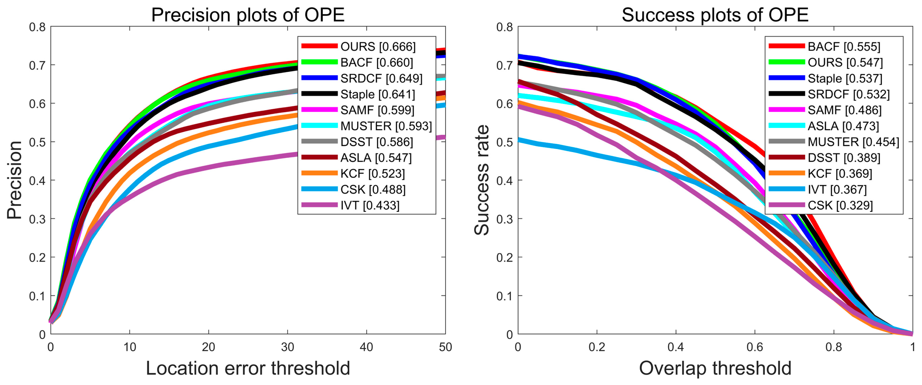
| OURS | 66.6% | 54.7% | 60.7% |
| Staple | 64.1% | 53.7% | 58.9% |
| BACF | 66.0% | 55.5% | 60.8% |
| SRDCF | 64.9% | 53.2% | 59.1% |
| SAMF | 59.9% | 48.6% | 54.3% |
| KCF | 52.3% | 36.9% | 44.6% |
| DSST | 58.6% | 38.9% | 48.8% |
| CSK | 48.8% | 32.2% | 40.5% |
| MUSTER | 59.3% | 45.4% | 52.4% |
| ASLA | 54.7% | 47.3% | 51.0% |
| TVT | 43.3% | 36.7% | 40.0% |
Publisher’s Note: MDPI stays neutral with regard to jurisdictional claims in published maps and institutional affiliations. |
© 2022 by the authors. Licensee MDPI, Basel, Switzerland. This article is an open access article distributed under the terms and conditions of the Creative Commons Attribution (CC BY) license (https://creativecommons.org/licenses/by/4.0/).
Share and Cite
Liu, C.; Ibrayim, M.; Hamdulla, A. Multi-Feature Single Target Robust Tracking Fused with Particle Filter. Sensors 2022, 22, 1879. https://doi.org/10.3390/s22051879
Liu C, Ibrayim M, Hamdulla A. Multi-Feature Single Target Robust Tracking Fused with Particle Filter. Sensors. 2022; 22(5):1879. https://doi.org/10.3390/s22051879
Chicago/Turabian StyleLiu, Caihong, Mayire Ibrayim, and Askar Hamdulla. 2022. "Multi-Feature Single Target Robust Tracking Fused with Particle Filter" Sensors 22, no. 5: 1879. https://doi.org/10.3390/s22051879
APA StyleLiu, C., Ibrayim, M., & Hamdulla, A. (2022). Multi-Feature Single Target Robust Tracking Fused with Particle Filter. Sensors, 22(5), 1879. https://doi.org/10.3390/s22051879