
Automatic Dynamic Range Adjustment for Pedestrian Detection in Thermal (Infrared) Surveillance Videos


Abstract
:1. Introduction
2. Related Works
3. Proposed Method
3.1. Dynamic Range Adjustment
| Algorithm 1: Dynamic Range Adjustment. |
 |
3.1.1. Histogram Specification Using Histogram Equalisation
3.1.2. Histogram Partitioning
3.2. Candidate Validation
4. Experimental Results and Discussion
4.1. Dataset
- OTCBVS benchmark—Ohio State University (OSU) thermal pedestrian database [39], which contains ten sessions of 360 × 240 thermal images of the walking intersection and street of the Ohio State University captured during both day and night over many days under a variety of environmental conditions culminating in a total of 284 frames, each having an average of three to four people. The images were captured using Raytheon 300D thermal sensor with a 75 mm lens camera mounted on an eight-storey building.
- LITIV dataset [40], which contains nine sequences of 320 × 240 thermal videos captured at 30 frames per second with different zoom settings from relatively high altitudes and at different positions culminating in a total of 6325 frames of lengths varying between 11 s and 88 s.
- OTCBVS benchmark—Terravic Motion IR database [41], which features 18 thermal sequences with 8-bit grayscale JPEG images of size 320 × 240 pixels taken with a Raytheon L-3 Thermal Eye. Eleven sequences were chosen from the Outdoor Motion and Tracking (OMT) Scenarios.
- The Linkoping Thermal InfraRed (LTIR) dataset [42], which consists of 20 thermal infrared sequences featured in the Visual Object Recognition (VOT) challenge 2015. Four sequences pertaining to pedestrian detection were chosen: Saturated, Street, Crossing, and Hiding.
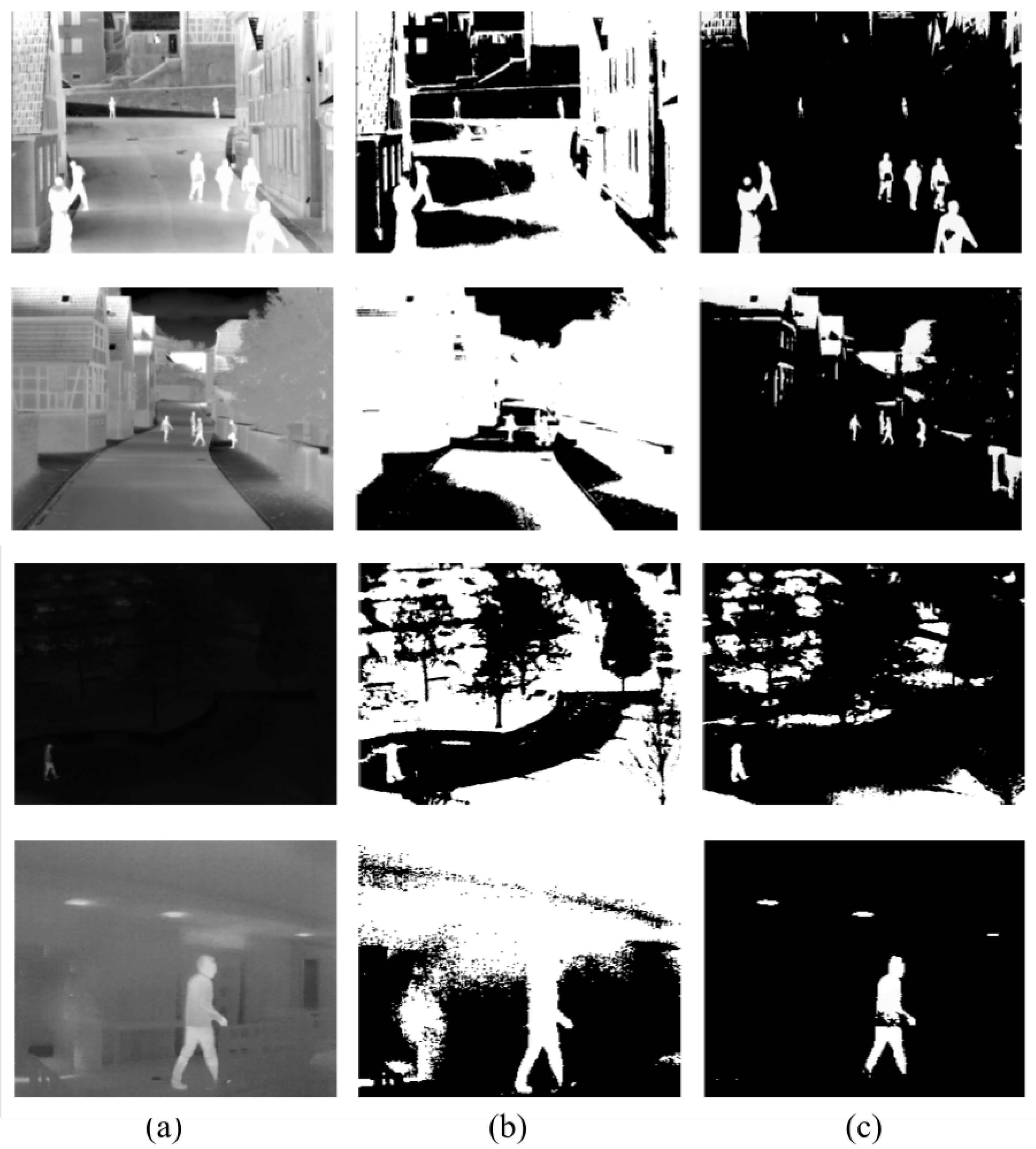
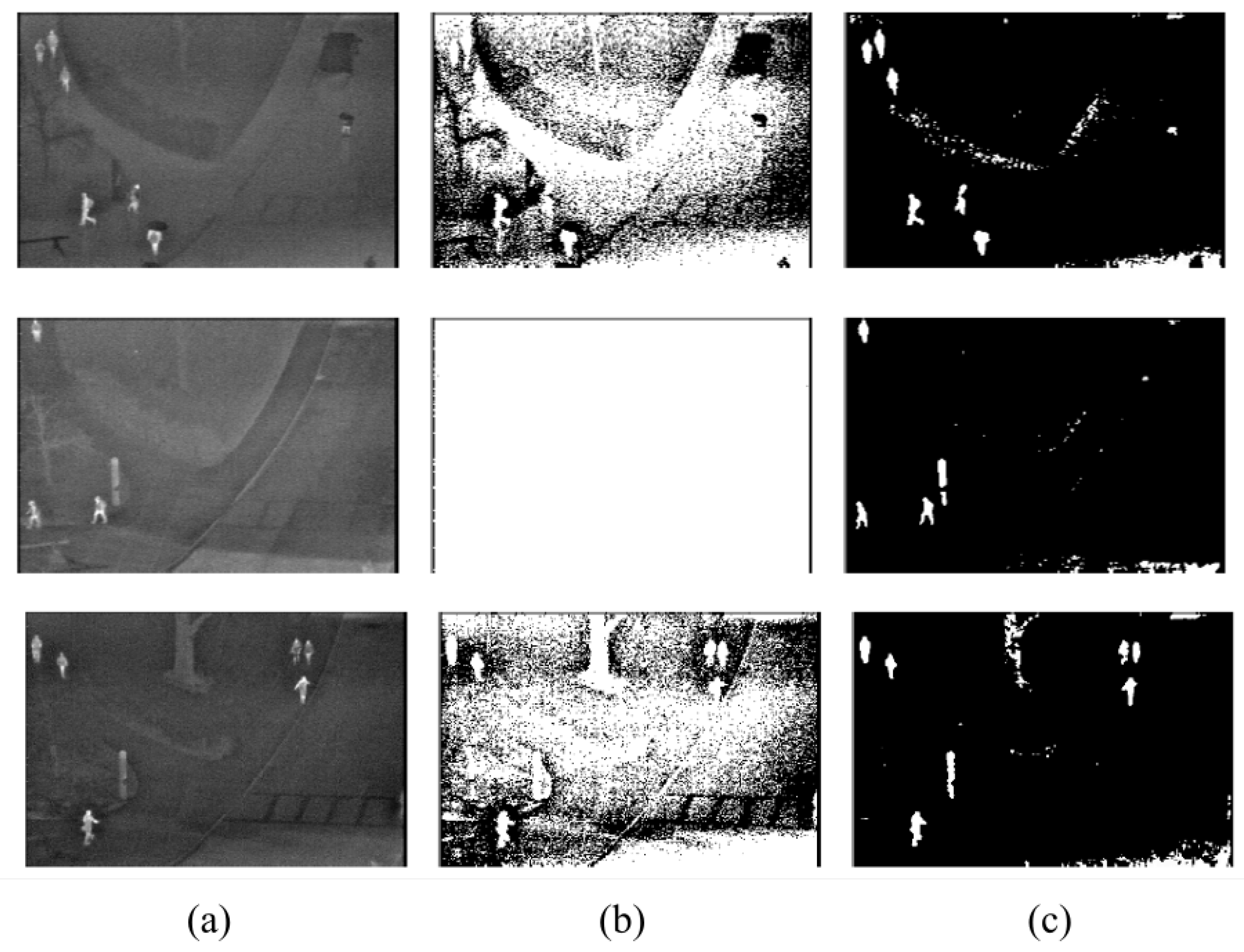
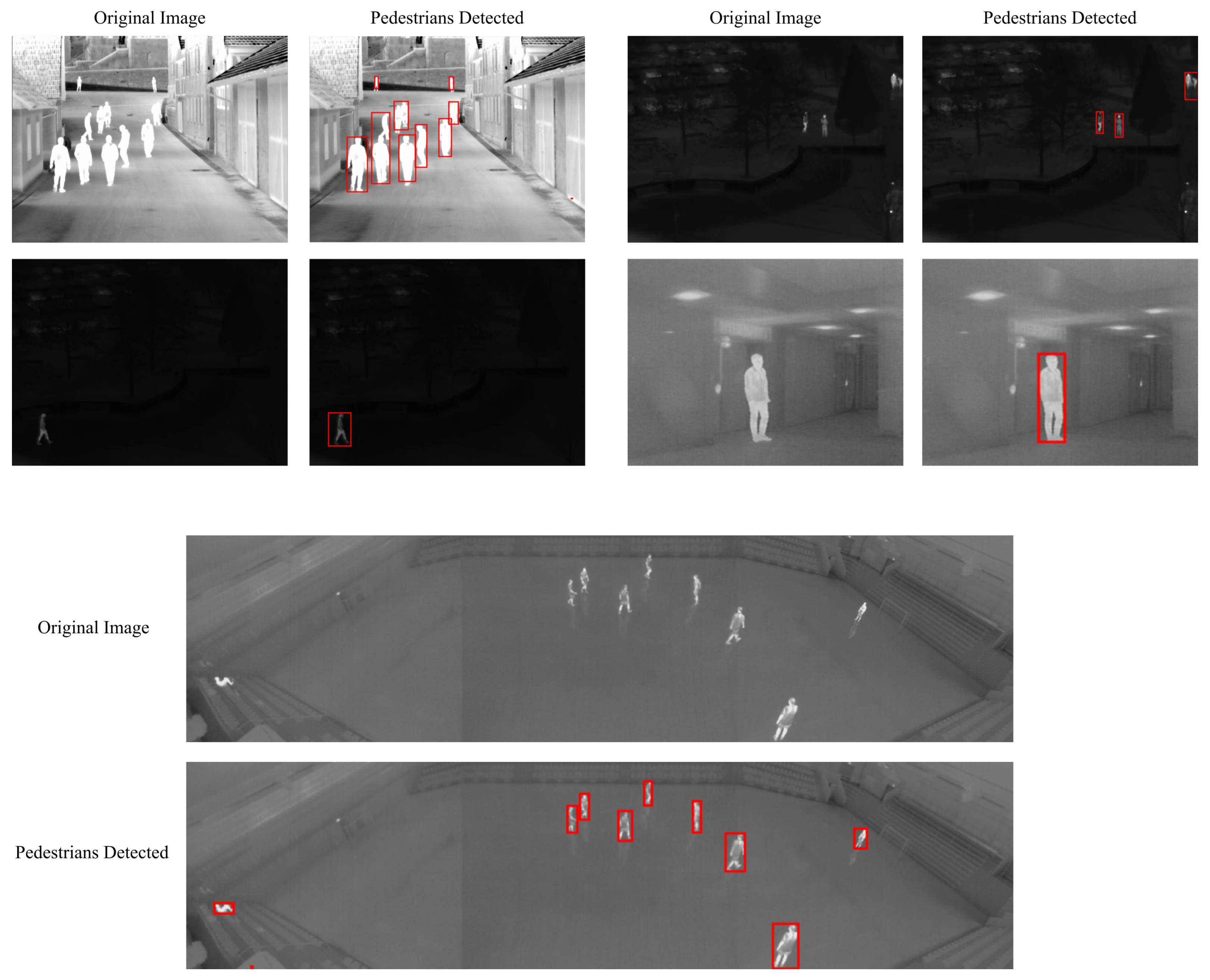
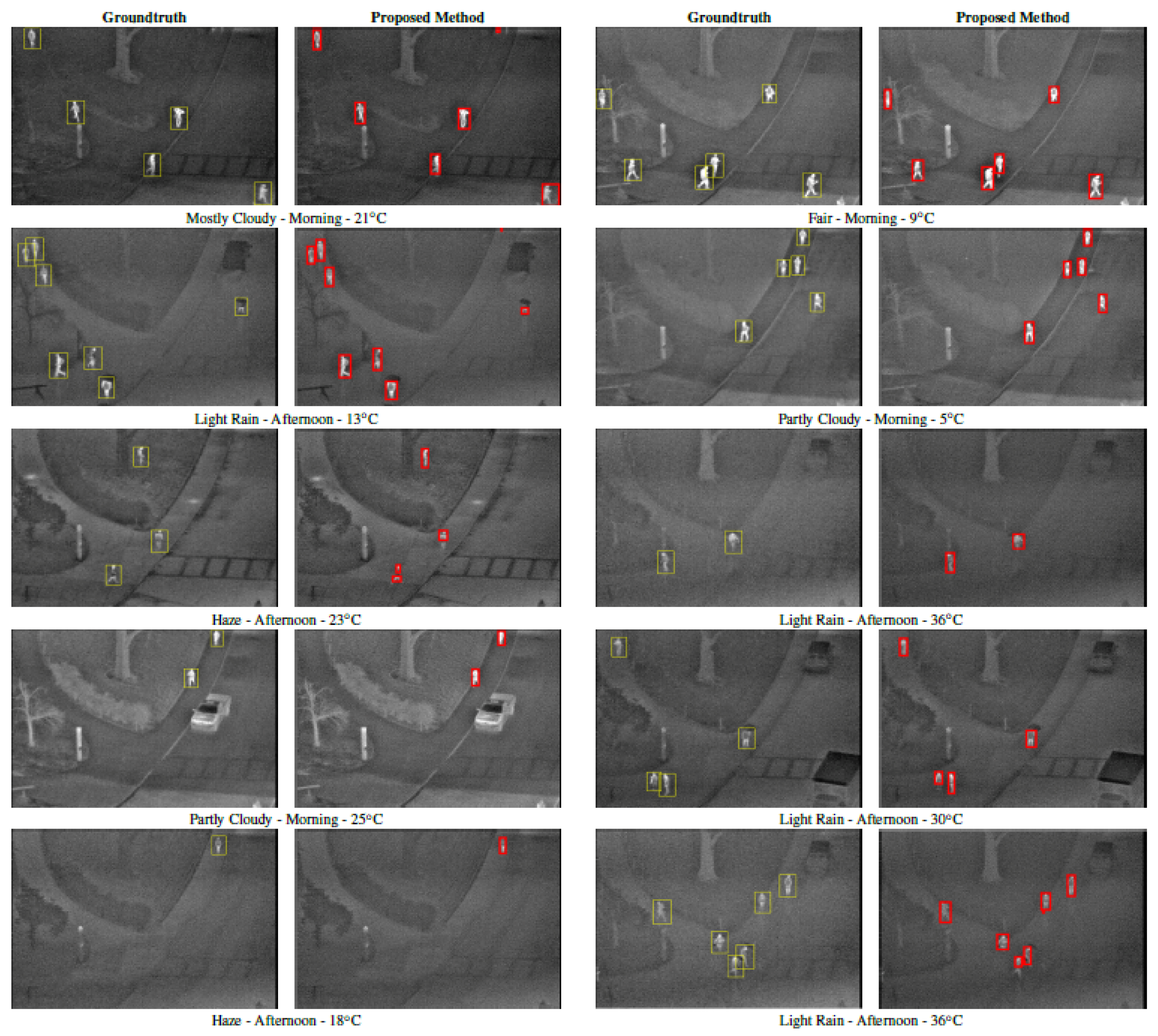
4.2. Qualitative Performance Evaluation
4.3. Quantitative Performance Evaluation
5. Conclusions
Author Contributions
Funding
Data Availability Statement
Conflicts of Interest
References
- Fluke. Hot Spot Detection—What to Look For. 2020. Available online: https://www.fluke.com/en/learn/blog/thermal-imaging/hot-spot-detection (accessed on 8 May 2012).
- Stuart, M. A Practical Guide to Emissivity in Infrared Inspections. Uptime. 2016, pp. 43–46. Available online: https://reliabilityweb.com/articles/entry/a-practical-guide-to-emissivity-in-infrared-inspections (accessed on 21 January 2022).
- Cook, D. Thermal Images. Available online: https://www.robotroom.com/Flir-Infrared-Camera-4.html (accessed on 21 January 2022).
- Otsu, N. A Threshold Selection Method from Gray-Level Histograms. IEEE Trans. Syst. Man Cybern. 1979, 9, 62–66. [Google Scholar] [CrossRef] [Green Version]
- Pun, T. A new method for grey-level picture thresholding using the entropy of the histogram. Signal Process. 1980, 2, 223–237. [Google Scholar] [CrossRef]
- Li, C.; Lee, C. Minimum cross entropy thresholding. Pattern Recognit. 1993, 26, 617–625. [Google Scholar] [CrossRef]
- Itti, L.; Koch, C.; Niebur, E. A model of saliency-based visual attention for rapid scene analysis. IEEE Trans. Pattern Anal. Mach. Intell. 1998, 20, 1254–1259. [Google Scholar] [CrossRef] [Green Version]
- Hou, Z.; Hu, Q.; Nowinski, W.L. On Minimum Variance Thresholding. Pattern Recogn. Lett. 2006, 27, 1732–1743. [Google Scholar] [CrossRef]
- Harel, J.; Koch, C.; Perona, P. Graph-Based Visual Saliency. In Proceedings of the 19th International Conference on Neural Information Processing Systems, Vancouver, BC, Canada, 4–7 December 2006; MIT Press: Cambridge, MA, USA, 2006; pp. 545–552. [Google Scholar]
- Achanta, R.; Hemami, S.; Estrada, F.; Susstrunk, S. Frequency-tuned salient region detection. In Proceedings of the 2009 IEEE Conference on Computer Vision and Pattern Recognition, Miami, FL, USA, 20–25 June 2009; pp. 1597–1604. [Google Scholar]
- Chaki, N.; Shaikh, S.H.; Saeed, K. A comprehensive survey on image binarization techniques. In Exploring Image Binarization Techniques; Springer: New Delhi, India, 2014; pp. 5–15. [Google Scholar]
- Shaikh, S.H.; Saeed, K.; Chaki, N. Moving object detection: A new approach. In Moving Object Detection Using Background Subtraction; Springer: Cham, Switzerland, 2014; pp. 25–48. [Google Scholar]
- Soundrapandiyan, R.; Mouli, C. Adaptive Pedestrian Detection in Infrared Images using Background Subtraction and Local Thresholding. Procedia Comput. Sci. 2015, 58, 706–713. [Google Scholar] [CrossRef] [Green Version]
- Jeon, E.S.; Choi, J.S.; Lee, J.H.; Shin, K.Y.; Kim, Y.G.; Le, T.T.; Park, K.R. Human Detection Based on the Generation of a Background Image by Using a Far-Infrared Light Camera. Sensors 2015, 15, 6763–6787. [Google Scholar] [CrossRef] [Green Version]
- Jeyabharathi, D.; Dejey. Efficient background subtraction for thermal images using reflectional symmetry pattern (RSP). Multimed. Tools Appl. 2018, 77, 22567–22586. [Google Scholar] [CrossRef]
- Ma, M. Infrared pedestrian detection algorithm based on multimedia image recombination and matrix restoration. Multimed. Tools Appl. 2020, 79, 9267–9282. [Google Scholar] [CrossRef]
- Soundrapandiyan, R.; Mouli, C.P. An Approach to Adaptive Pedestrian Detection and Classification in Infrared Images Based on Human Visual Mechanism and Support Vector Machine. Arab. J. Sci. Eng. 2018, 43, 3951–3963. [Google Scholar] [CrossRef]
- Wu, T.; Hou, R.; Chen, Y. Cloud Model-Based Method for Infrared Image Thresholding. Math. Probl. Eng. 2016, 2016, 1571795. [Google Scholar] [CrossRef] [Green Version]
- Manda, M.P.; Park, C.; Oh, B.; Hyun, D.; Kim, H.S. Pedestrian Detection in Infrared Thermal Images Based on Raised Cosine Distribution. In Proceedings of the 2020 International SoC Design Conference (ISOCC), Yeosu, Korea, 21–24 October 2020; pp. 278–279. [Google Scholar]
- Manda, M.P.; Kim, H.S. A Fast Image Thresholding Algorithm for Infrared Images Based on Histogram Approximation and Circuit Theory. Algorithms 2020, 13, 207. [Google Scholar] [CrossRef]
- Zhao, Y.; Cheng, J.; Zhou, W.; Zhang, C.; Pan, X. Infrared Pedestrian Detection with Converted Temperature Map. In Proceedings of the 2019 Asia-Pacific Signal and Information Processing Association Annual Summit and Conference (APSIPA ASC), Lanzhou, China, 18–21 November 2019; pp. 2025–2031. [Google Scholar]
- Dai, X.; Duan, Y.; Hu, J.; Liu, S.; Hu, C.; He, Y.; Chen, D.; Luo, C.; Meng, J. Near infrared nighttime road pedestrians recognition based on convolutional neural network. Infrared Phys. Technol. 2019, 97, 25–32. [Google Scholar] [CrossRef]
- Gao, Z.; Zhang, Y.; Li, Y. Extracting features from infrared images using convolutional neural networks and transfer learning. Infrared Phys. Technol. 2020, 105, 103237. [Google Scholar] [CrossRef]
- Huda, N.U.; Hansen, B.D.; Gade, R.; Moeslund, T.B. The Effect of a Diverse Dataset for Transfer Learning in Thermal Person Detection. Sensors 2020, 20, 1982. [Google Scholar] [CrossRef] [Green Version]
- Krišto, M.; Ivasic-Kos, M.; Pobar, M. Thermal Object Detection in Difficult Weather Conditions Using YOLO. IEEE Access 2020, 8, 125459–125476. [Google Scholar] [CrossRef]
- Tumas, P.; Nowosielski, A.; Serackis, A. Pedestrian Detection in Severe Weather Conditions. IEEE Access 2020, 8, 62775–62784. [Google Scholar] [CrossRef]
- Haider, A.; Shaukat, F.; Mir, J. Human detection in aerial thermal imaging using a fully convolutional regression network. Infrared Phys. Technol. 2021, 116, 103796. [Google Scholar] [CrossRef]
- My, K.; Berlincioni, L.; Galteri, L.; Bertini, M.; Bagdanov, A.; Bimbo, A. Robust pedestrian detection in thermal imagery using synthesized images. In Proceedings of the 2020 25th International Conference on Pattern Recognition, Milan, Italy, 10–15 January 2021. [Google Scholar]
- LI, S.; Li, Y.; Li, Y.; Li, M.; Xu, X. YOLO-FIRI: Improved YOLOv5 for Infrared Image Object Detection. IEEE Access 2021, 9, 141861–141875. [Google Scholar] [CrossRef]
- Pal, N.R. On minimum cross-entropy thresholding. Pattern Recognit. 1996, 29, 575–580. [Google Scholar] [CrossRef]
- Brink, A.; Pendock, N. Minimum cross-entropy threshold selection. Pattern Recognit. 1996, 29, 179–188. [Google Scholar] [CrossRef]
- Al-Osaimi, G.; El-Zaart, A. Minimum Cross Entropy Thresholding for SAR Images. In Proceedings of the 2008 3rd International Conference on Information and Communication Technologies: From Theory to Applications, Damascus, Syria, 7–11 April 2008; pp. 1–6. [Google Scholar]
- Lei, B.; Fan, J. Multilevel minimum cross entropy thresholding: A comparative study. Appl. Soft Comput. 2020, 96, 106588. [Google Scholar] [CrossRef]
- Coltuc, D.; Bolon, P.; Chassery, J.M. Exact histogram specification. IEEE Trans. Image Process. 2006, 15, 1143–1152. [Google Scholar] [CrossRef] [PubMed]
- Shannon, C.E. A Mathematical Theory of Communication. Bell Syst. Tech. J. 1948, 27, 379–423. [Google Scholar] [CrossRef] [Green Version]
- Shore, J.; Johnson, R. Axiomatic derivation of the principle of maximum entropy and the principle of minimum cross-entropy. IEEE Trans. Inf. Theory 1980, 26, 26–37. [Google Scholar] [CrossRef] [Green Version]
- Murphy, K.P. Machine Learning: A Probabilistic Perspective; The MIT Press: Cambridge, MA, USA, 2012. [Google Scholar]
- Frieden, B.R. Restoring with Maximum Likelihood and Maximum Entropy. J. Opt. Soc. Am. 1972, 62, 511–518. [Google Scholar] [CrossRef] [PubMed]
- Davis, J.W.; Keck, M.A. A Two-Stage Template Approach to Person Detection in Thermal Imagery. In Proceedings of the Seventh IEEE Workshop on Applications of Computer Science, WACV/MOTION’05, Breckenridge, CO, USA, 5–7 January 2005. [Google Scholar]
- Torabi, A.; Masse, G.; Bilodeau, G.A. An iterative integrated framework for thermal–visible image registration, sensor fusion, and people tracking for video surveillance applications. Comput. Vis. Image Underst. 2012, 116, 210–221. [Google Scholar] [CrossRef]
- Miezianko, R. IEEE OTCBVS WS Series Bench; Terravic Research Infrared Database. 2005. Available online: http://vcipl-okstate.org/pbvs/bench/Data/05/download.html (accessed on 21 January 2022).
- Berg, A.; Ahlberg, J.; Felsberg, M. A thermal Object Tracking benchmark. In Proceedings of the 2015 12th IEEE International Conference on Advanced Video and Signal Based Surveillance (AVSS), Karlsruhe, Germany, 25–28 August 2015; pp. 1–6. [Google Scholar]
- Oluyide, O.M.; Tapamo, J.; Walingo, T. Fast Background Subtraction and Graph Cut for Thermal Pedestrian Detection. In Pattern Recognition—13th Mexican Conference, MCPR 2021, Mexico City, Mexico, 23–26 June 2021; Lecture Notes in Computer Science; Springer: Cham, Switzerland, 2021; Volume 12725, pp. 219–228. [Google Scholar]


| Session | Cloud Condition | TOD | UV | Temp. (°C) |
|---|---|---|---|---|
| 1 | Light Rain | Afternoon | 1 | 13 |
| 2 | Partly Cloudy | Morning | 1 | 5 |
| 4 | Fair | Morning | 4 | 9 |
| 5 | Partly Cloudy | Morning | 1 | 25 |
| 6 | Mostly Cloudy | Morning | 1 | 21 |
| 7 | Light Rain | Afternoon | 1 | 36 |
| 8 | Light Rain | Afternoon | 2 | 30 |
| 9 | Haze | Afternoon | 0 | 18 |
| 10 | Haze | Afternoon | 2 | 23 |
| Session | #People | #TP | #FP | Precision | Recall |
|---|---|---|---|---|---|
| 1 | 91 | 88 | 0 | ||
| 2 | 100 | 100 | 0 | ||
| 4 | 109 | 109 | 0 | ||
| 5 | 101 | 101 | 2 | ||
| 6 | 97 | 94 | 0 | ||
| 7 | 80 | 93 | 1 | ||
| 8 | 96 | 98 | 0 | ||
| 9 | 95 | 95 | 0 | ||
| 10 | 97 | 89 | 0 |
| #TP | #FP | ||||||||||
|---|---|---|---|---|---|---|---|---|---|---|---|
| #Ped | [39] | [21] | [19] | [43] | Ours | [39] | [21] | [19] | [43] | Ours | |
| 1 | 91 | 88 | 77 | 78 | 85 | 88 | 0 | 3 | 0 | 0 | 0 |
| 2 | 100 | 94 | 99 | 98 | 97 | 100 | 0 | 2 | 2 | 2 | 0 |
| 4 | 109 | 107 | 107 | 109 | 109 | 109 | 1 | 7 | 10 | 0 | 0 |
| 5 | 101 | 90 | 97 | 101 | 97 | 101 | 0 | 16 | 16 | 1 | 2 |
| 6 | 97 | 93 | 92 | 97 | 93 | 94 | 0 | 8 | 0 | 0 | 0 |
| 7 | 94 | 92 | 78 | 80 | 90 | 93 | 0 | 8 | 0 | 1 | 1 |
| 8 | 99 | 75 | 89 | 96 | 93 | 98 | 1 | 8 | 0 | 0 | 0 |
| 9 | 95 | 95 | 91 | 95 | 95 | 95 | 0 | 4 | 16 | 0 | 0 |
| 10 | 97 | 95 | 91 | 83 | 89 | 89 | 3 | 18 | 6 | 0 | 0 |
| 1–10 | 883 | 829 | 821 | 837 | 848 | 867 | 5 | 74 | 50 | 4 | 3 |
| Method | Precision | Recall |
|---|---|---|
| [25] | ||
| [24] | ||
| [27] | ||
| Ours |
| Database | Sequence | Precision | Recall |
|---|---|---|---|
| LTIR | Saturated | ||
| LTIR | Street | ||
| LTIR | Crossing | ||
| LTIR | Hiding | ||
| LITIV | All | ||
| Terravic | 11 (OMT) | ||
| OSU | All |
Publisher’s Note: MDPI stays neutral with regard to jurisdictional claims in published maps and institutional affiliations. |
© 2022 by the authors. Licensee MDPI, Basel, Switzerland. This article is an open access article distributed under the terms and conditions of the Creative Commons Attribution (CC BY) license (https://creativecommons.org/licenses/by/4.0/).
Share and Cite
Oluyide, O.M.; Tapamo, J.-R.; Walingo, T.M. Automatic Dynamic Range Adjustment for Pedestrian Detection in Thermal (Infrared) Surveillance Videos. Sensors 2022, 22, 1728. https://doi.org/10.3390/s22051728
Oluyide OM, Tapamo J-R, Walingo TM. Automatic Dynamic Range Adjustment for Pedestrian Detection in Thermal (Infrared) Surveillance Videos. Sensors. 2022; 22(5):1728. https://doi.org/10.3390/s22051728
Chicago/Turabian StyleOluyide, Oluwakorede Monica, Jules-Raymond Tapamo, and Tom Mmbasu Walingo. 2022. "Automatic Dynamic Range Adjustment for Pedestrian Detection in Thermal (Infrared) Surveillance Videos" Sensors 22, no. 5: 1728. https://doi.org/10.3390/s22051728
APA StyleOluyide, O. M., Tapamo, J.-R., & Walingo, T. M. (2022). Automatic Dynamic Range Adjustment for Pedestrian Detection in Thermal (Infrared) Surveillance Videos. Sensors, 22(5), 1728. https://doi.org/10.3390/s22051728