Inpainted Image Reconstruction Using an Extended Hopfield Neural Network Based Machine Learning System


Abstract
:1. Introduction
2. Materials and Methods
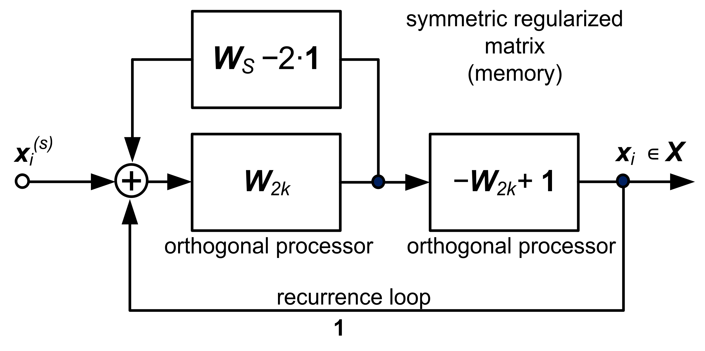
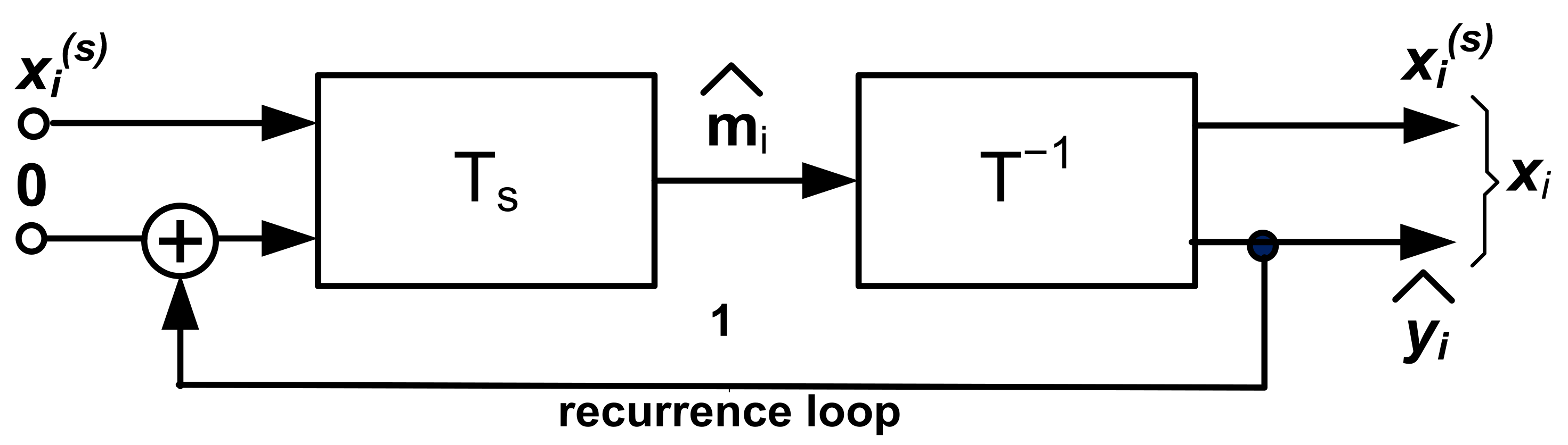
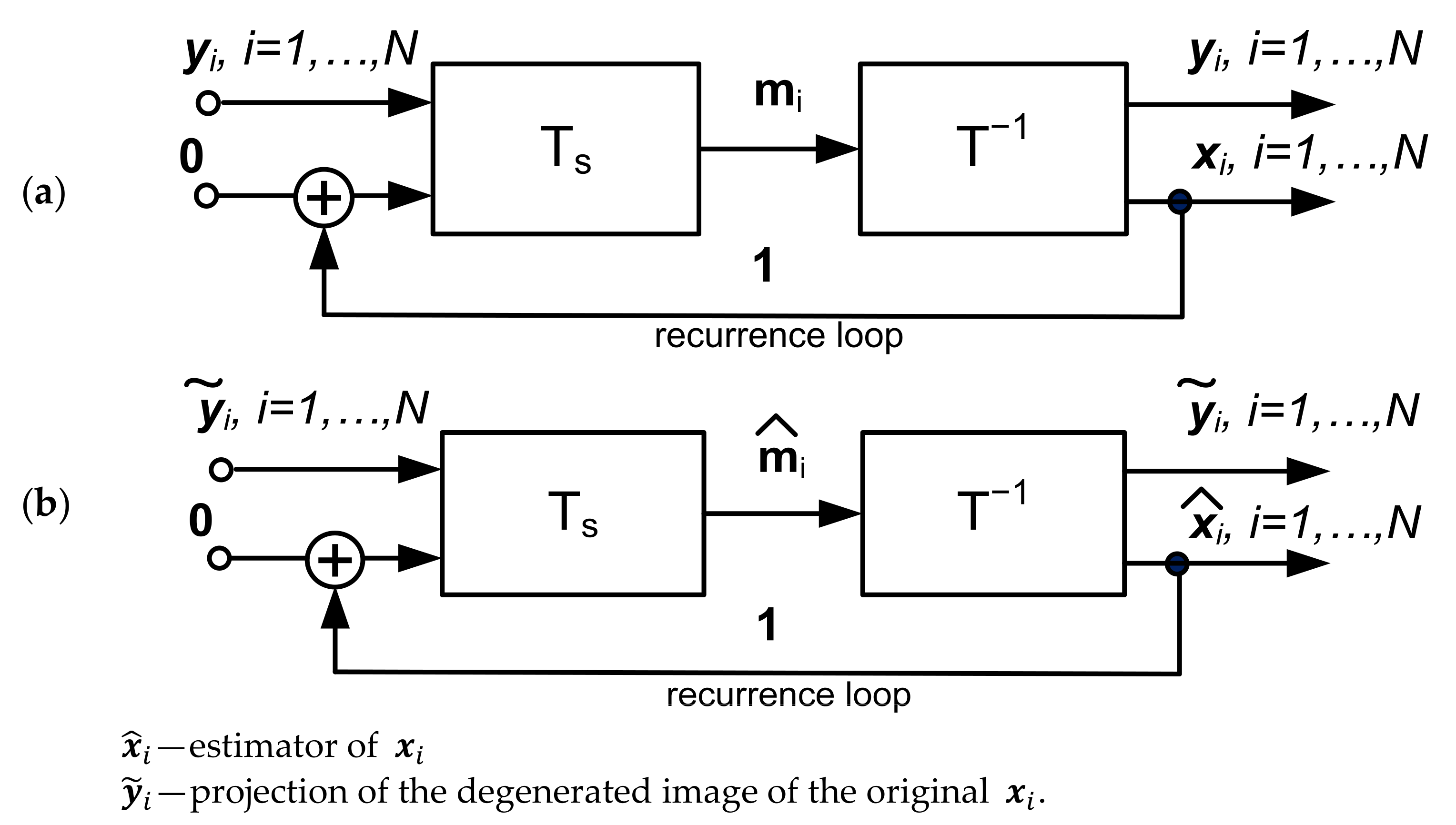
2.1. Machine Learning System for Image Processing
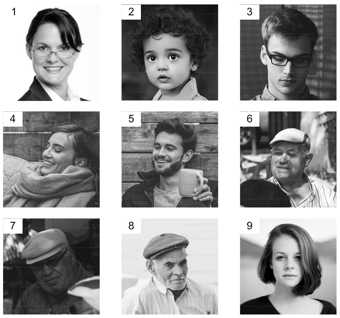
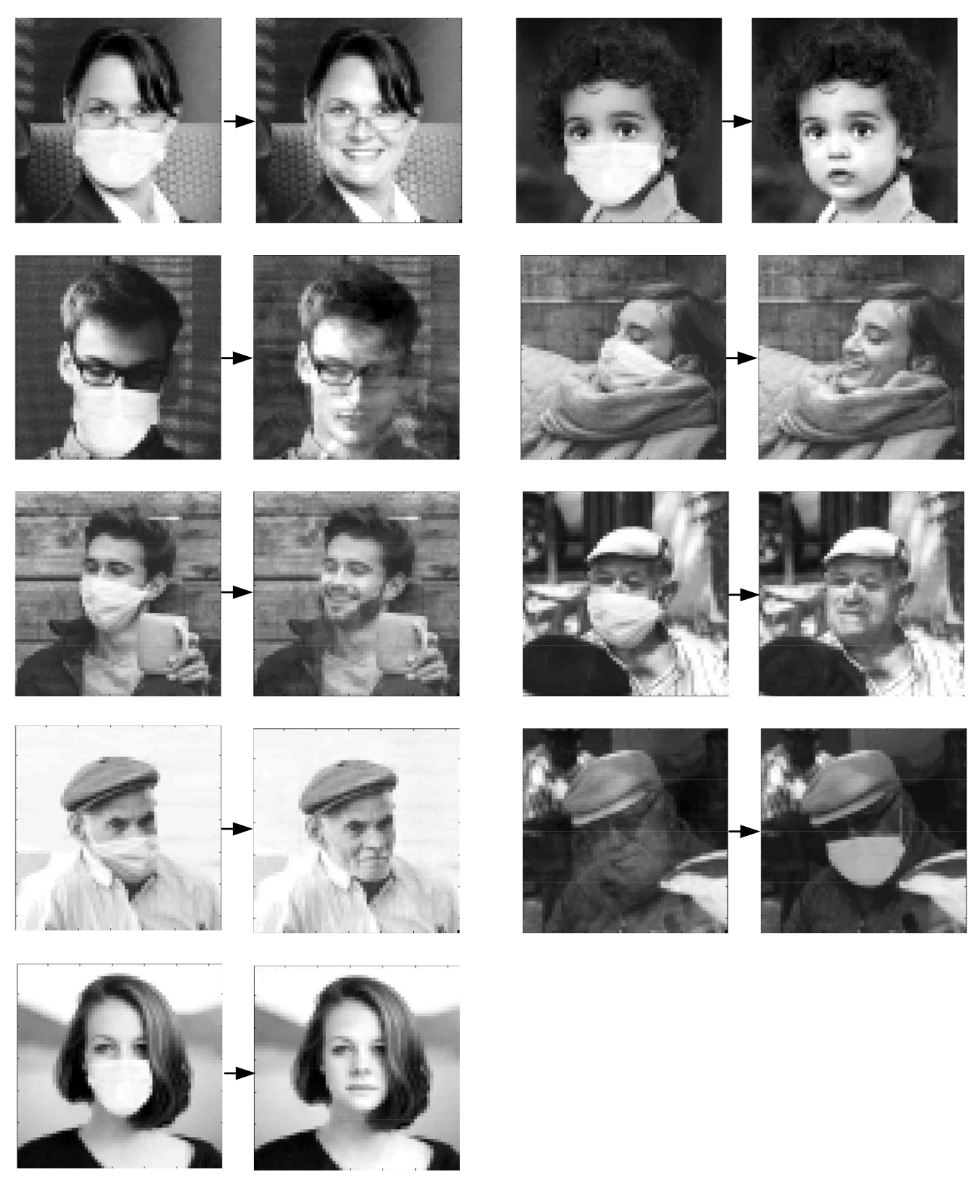
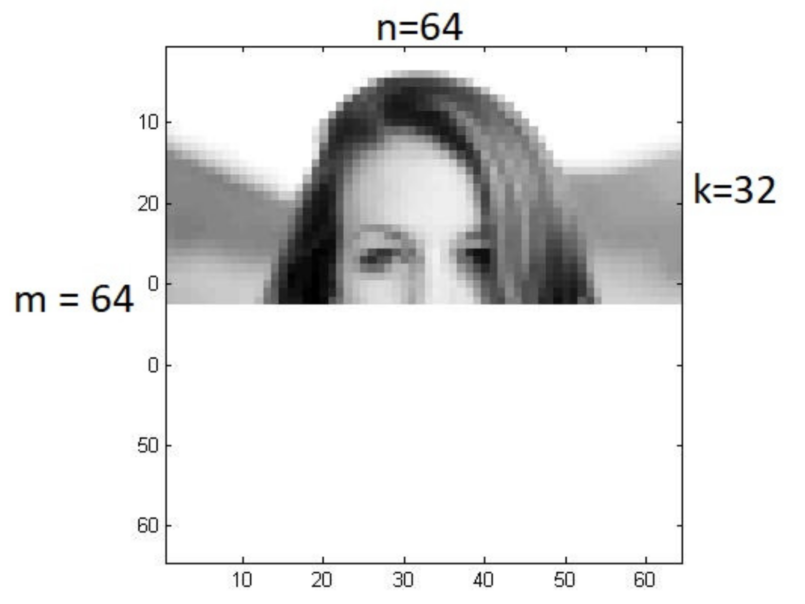
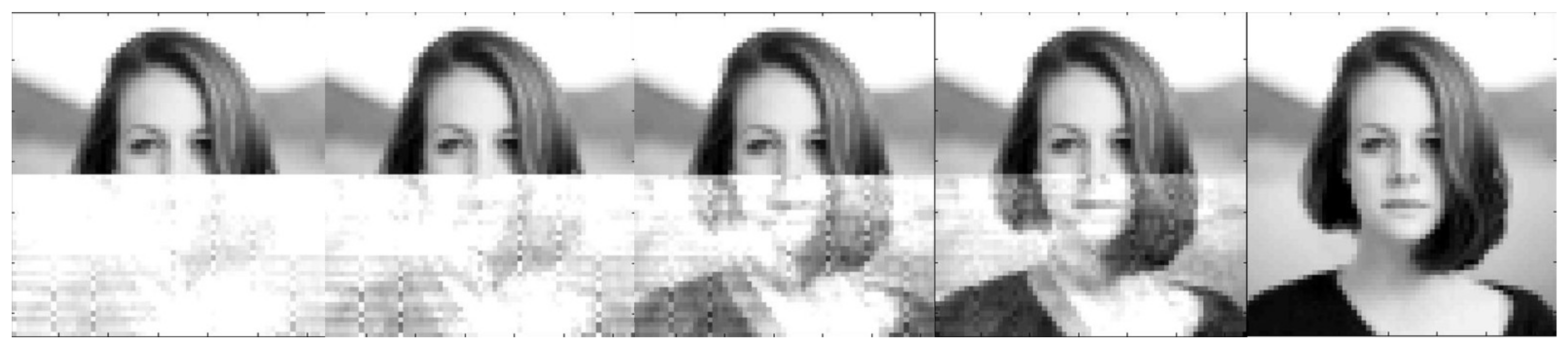
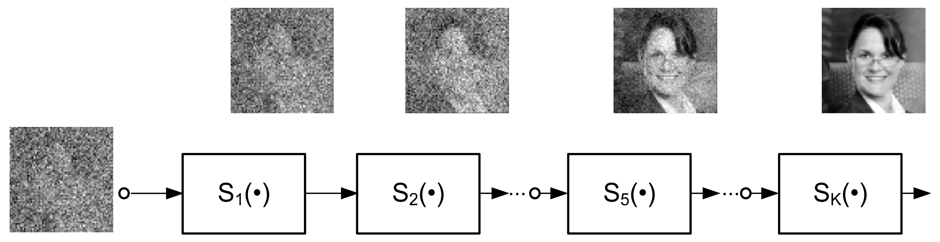
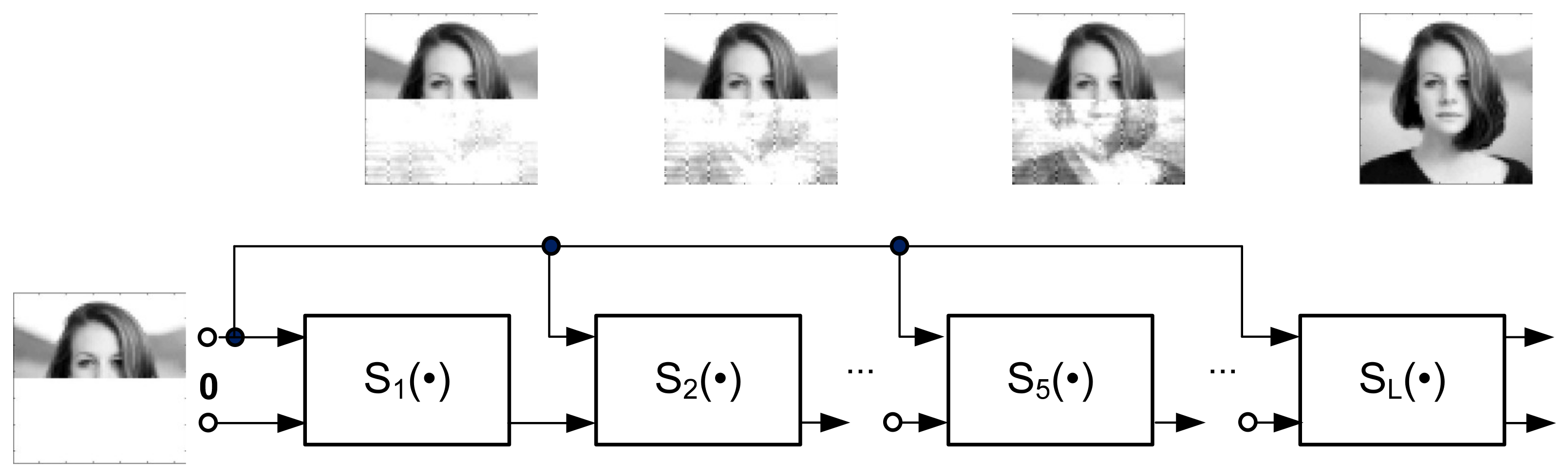
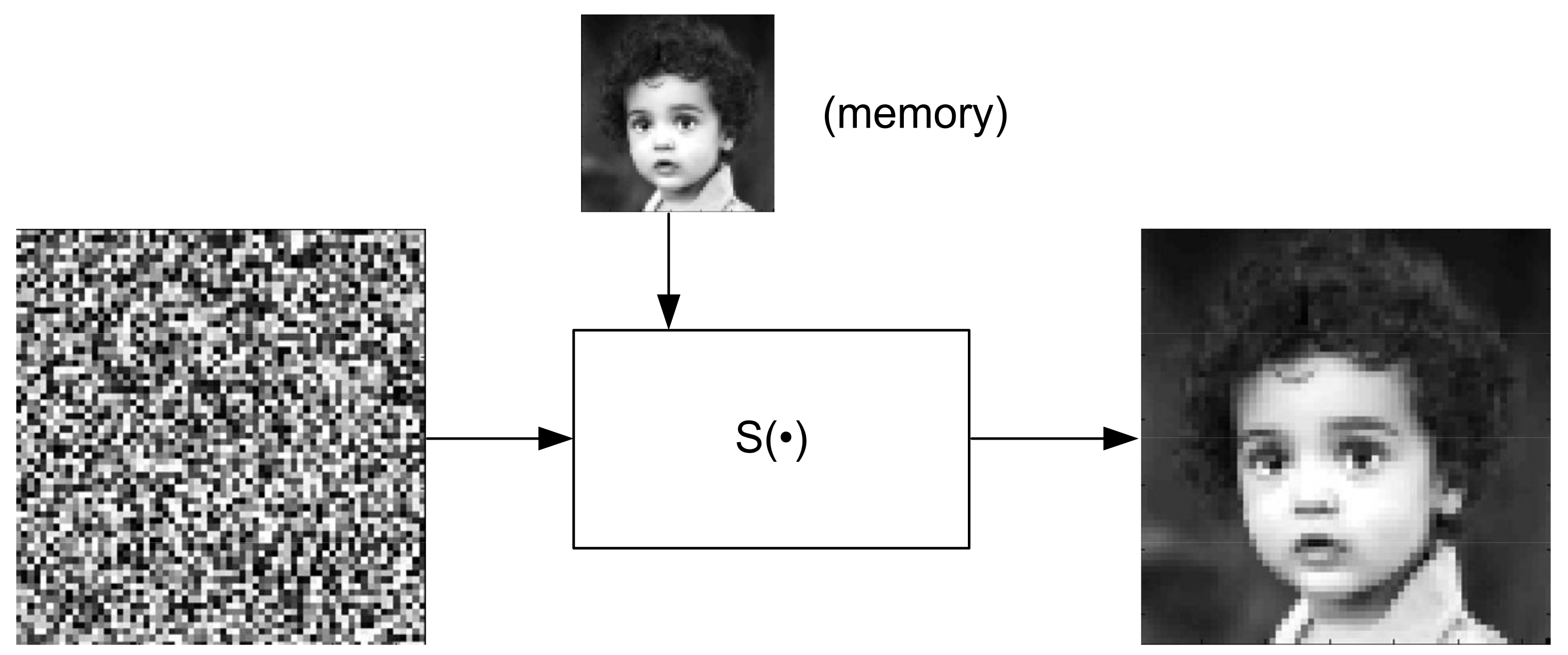
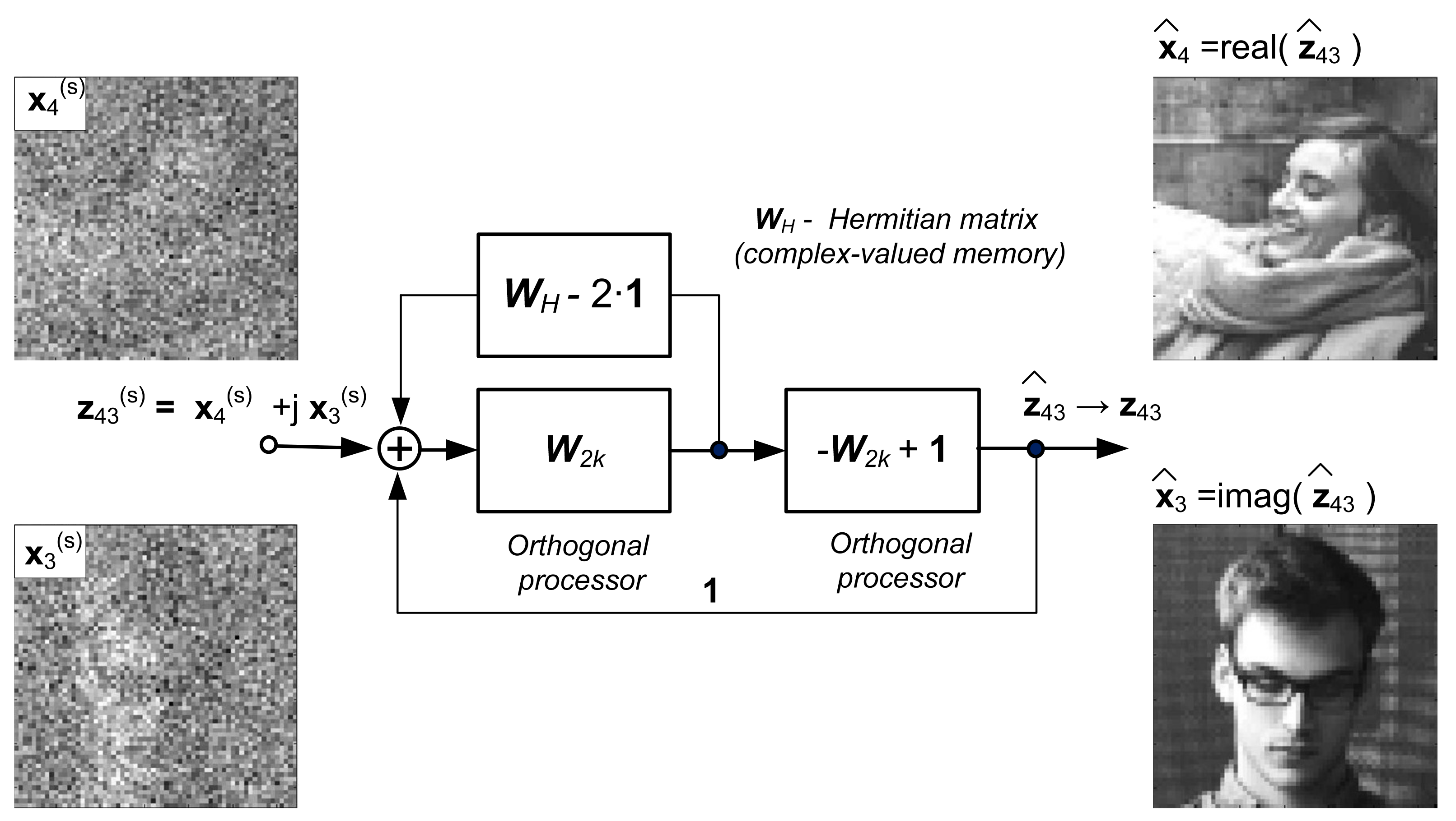
2.2. Computational Verification of the Learning Algorithm—Examples of Face Image Reconstruction and Person Recognition
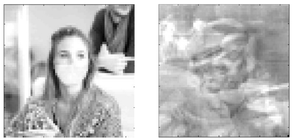
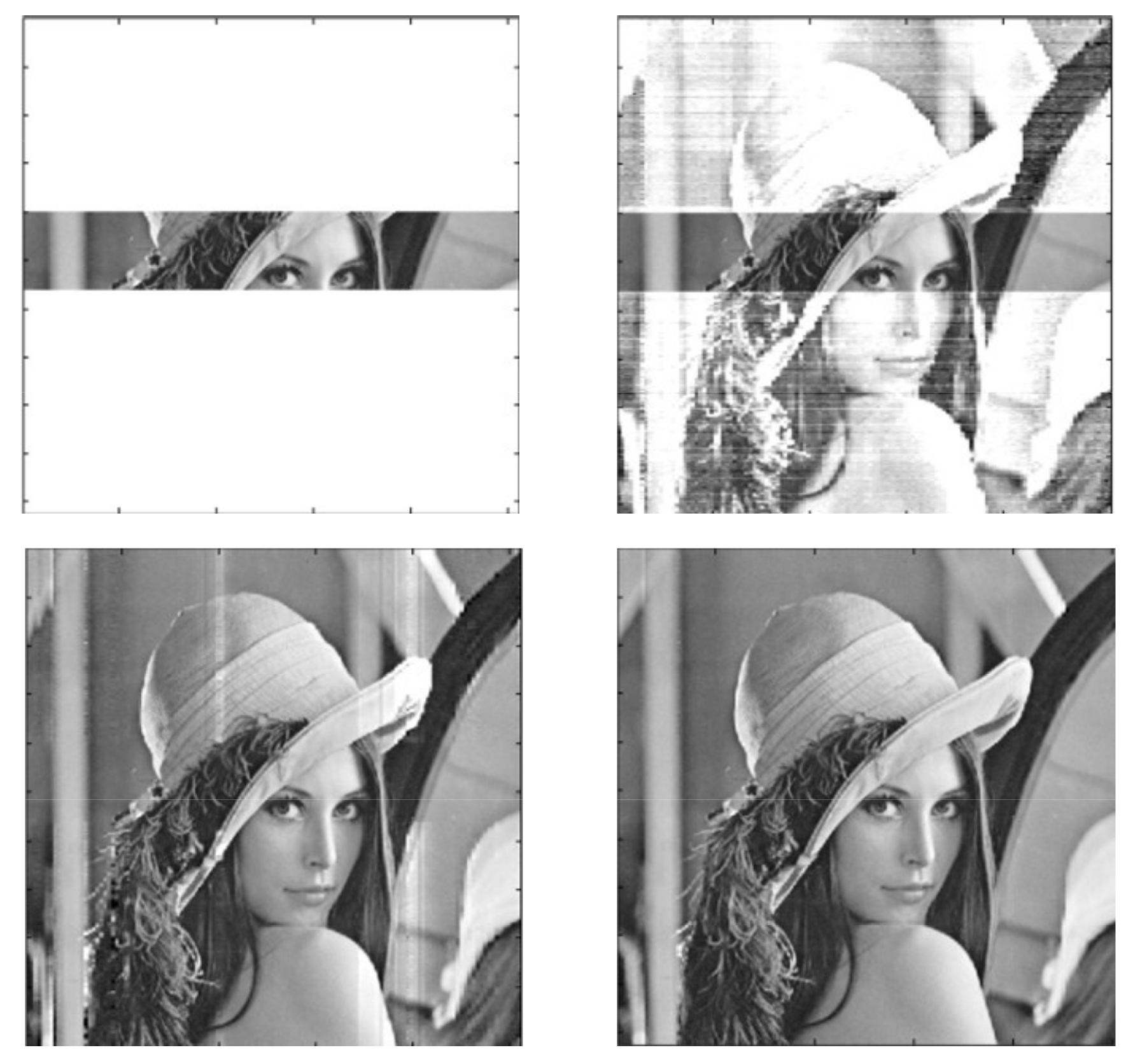
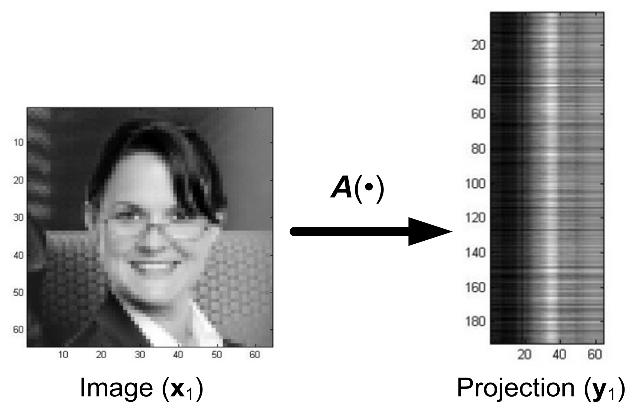
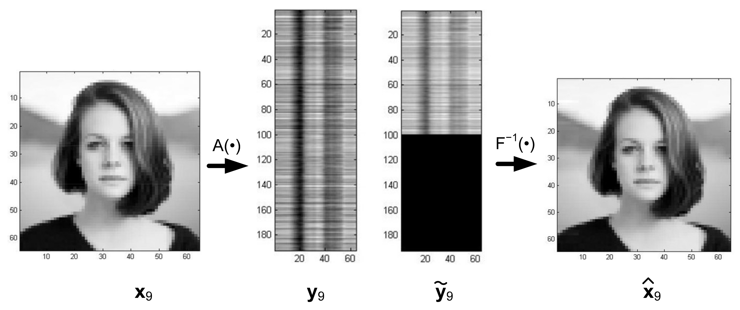
3. Inpainted Image Recognition and Reconstruction as an Inverse Problem
- —known processing operator, for example, is a matrix;
- —original image; and
- —observed degenerate image.
- K—set of feasible solutions;
- —regulizer;
- regularization parameter.
- known real matrix, ;
- real matrix;
- real matrix;
4. Discussion on Some Features of the Machine Learning System
5. Conclusions
Author Contributions
Funding
Institutional Review Board Statement
Informed Consent Statement
Data Availability Statement
Conflicts of Interest
Appendix A
| Algorithm A1. Summary of algorithm [1]. |
|
| Input the set of training points: |
| , |
|
| Create system vectors |
| . |
| Calculate the spectrum of system vectors |
| Create spectrum matrix |
| Calculate Hermitian matrix : |
| Calculate orthogonal transformation : |
| Calculate biorthogonal transformation : |
| . |
|
| for i = 1:N |
| while |
| end |
| end |
| ( steps of recurrence) |
| . |
References
- Citko, W.; Sienko, W. Hamiltonian and Q-Inspired Neural Network-Based Machine Learning. IEEE Access 2020, 8, 220437–220449. [Google Scholar] [CrossRef]
- Gonzales, R.C.; Woods, R.E. Digital Image Processing; Pearson International Edition; Pearson: London, UK, 2008. [Google Scholar]
- Nelson, R.A.; Roberts, R.G. Some Multilinear Variants of Principal Component Analysis: Examples in Grayscale Image Recognition and Reconstruction. IEEE Syst. Man Cybern. Mag. 2021, 7, 25–35. [Google Scholar] [CrossRef]
- Sirovich, L.; Kirby, M. Low Dimensional Procedure for the Characterization of Human Faces. J. Opt. Soc. Am. 1987, 4, 519–524. [Google Scholar] [CrossRef] [PubMed]
- Turk, M.; Pentland, A. Face Recognition Using Eigenfaces. In Proceedings of the IEEE Computer Society Conference on Computer Vision and Pattern Recognition (CVPR ’91), Maui, HI, USA, 3–6 June 1991; pp. 586–591. [Google Scholar]
- Pal, S.K.; Ghosh, A.; Kundu, M.K. (Eds.) Soft Computing for Image Processing. In Studies in Fuzziness and Soft Computing; Physica-Verlang Heidelberg: New York, NY, USA, 2000. [Google Scholar]
- Huang, Z.; Ye, S.; McCann, M.T.; Ravishankar, S. Model-based Reconstruction with Learning: From Unsupervised to Supervised and Beyond. arXiv 2021, arXiv:2103.14528v1. [Google Scholar]
- Kaderuppan, S.S.; Wong, W.W.L.; Sharma, A.; Woo, W.L. Smart Nanoscopy: A Review of Computational Approaches to Achieve Super-Resolved Optical Microscopy. IEEE Access 2020, 8, 214801–214831. [Google Scholar] [CrossRef]
- Ramanarayanan, S.; Murugesan, B.; Ram, K.; Sivaprakasam, M. DC-WCNN: A Deep Cascade of Wavelet Based Convolutional Neural Networks for MR Image Reconstruction. In Proceedings of the IEEE 17th International Symposium on Biomedical Imaging (ISBI), Iowa City, IA, USA, 3–7 April 2020. [Google Scholar]
- Ravishankar, S.; Lahiri, A.; Blocker, C.; Fessler, J.A. Deep Dictionary-transform Learning for Image Reconstruction. In Proceedings of the 2018 IEEE 15th International Symposium on Biomedical Imaging (ISBI 2018), Washington, DC, USA, 4–7 April 2018; pp. 1208–1212. [Google Scholar] [CrossRef]
- Ravishankar, S.; Ye, J.C.; Fessler, J.A. Image Reconstruction: From Sparsity to Data-Adaptive Methods and Machine Learning. Proc. IEEE 2020, 108, 86–109. [Google Scholar] [CrossRef] [PubMed] [Green Version]
- Ravishankar, S.; Bresler, Y. MR Image Reconstruction From Highly Undersampled k-Space Data by Dictionary Learning. IEEE Trans. Med. Imaging 2021, 30, 1028–1041. [Google Scholar] [CrossRef] [PubMed]
- Panagakis, Y.; Kossaifi, J.; Chrysos, G.G.; Oldfield, J.; Nicolaou, M.A.; Anandkumar, A.; Zafeiriou, S. Tensor Methods in Computer Vision and Deep Learning. Proc. IEEE 2021, 109, 863–890. [Google Scholar] [CrossRef]
- Fessler, A.J. Optimization Methods for Magnetic Resonance Image Reconstruction: Key Models and Optimization Algorithms. IEEE Signal Process. Mag. 2020, 37, 33–40. [Google Scholar] [CrossRef] [PubMed]
- Zheng, H.; Sherazi, S.W.A.; Son, S.H.; Lee, J.Y. A Deep Convolutional Neural Network-Based Multi-Class Image Classification for Automatic Wafer Map Failure Recognition in Semiconductor Manufacturing. Appl. Sci. 2021, 11, 9769. [Google Scholar] [CrossRef]
- Szhou, S.K.; Greenspan, H.; Davatzikos, C.; Duncan, J.S.; Ginneken, B.; Madabhushi, A.; Prince, J.L.; Rueckert, D.; Summers, R.M. A Review of Deep Learning in Medical Imaging: Imaging Traits, Technology Trends, Case Studies with Progress Highlights, and Future Promise. Proc. IEEE 2021, 109, 820–838. [Google Scholar]
- Quan, T.M.; Nguyen-Duc, T.; Jeong, W.K. Compressed Sensing MRI Reconstruction Using a Generative Adversarial Network with a Cyclic Loss. IEEE Trans. Med. Imaging 2018, 37, 1488–1497. [Google Scholar] [CrossRef] [PubMed] [Green Version]
- Mardani, M.; Gong, E.; Cheng, J.Y.; Vasanawala, S.S.; Zaharchuk, G.; Xing, L.; Pauly, J.M. Deep Generative Adversarial Neural Networks for compressive sensing MRI. IEEE Trans. Med. Imaging 2019, 38, 167–179. [Google Scholar] [CrossRef] [PubMed]
- Liang, D.; Cheng, J.; Ke, Z.; Ying, L. Deep Magnetic Resonance Image Reconstruction: Inverse Problems Meet Neural Networks. IEEE Signal Process. Mag. 2020, 37, 141–151. [Google Scholar] [CrossRef] [PubMed]
- Sienko, W.; Citko, W. Hamiltonian Neural Networks Based Networks for Learning. In Machine Learning; Mellouk, A., Chebira, A., Eds.; I-Tech: Vienna, Austria, 2009; pp. 75–92. [Google Scholar]
- Gilton, D.; Ongie, G.; Willett, R. Deep Equilibrium Architectures for Inverse Problems in Imaging. arXiv 2021, arXiv:2102.07944v2. [Google Scholar] [CrossRef]
- Arridge, S.; Maass, P.; Oktem, O.; Schonlieb, C. Solving Inverse Problems using Data-driven Models. Acta Numer. 2019, 28, 1–174. [Google Scholar] [CrossRef] [Green Version]
- Ongie, G.; Jalal, A.; Metzler, C.A.; Baraniuk, R.G.; Dimakis, A.G.; Willett, R. Deep Learning Techniques for Inverse Problems in Imaging. arXiv 2020, arXiv:205.06001. [Google Scholar] [CrossRef]
- Gilton, D.; Ongie, G.; Willett, R. Model Adaptation for Inverse Problems in Imaging. arXiv 2021, arXiv:2012.00139v2. [Google Scholar] [CrossRef]
- Giryes, R.; Eldar, Y.C.; Bronstein, A.M.; Sapiro, G. Tradeoffs Between Convergences Speed and Reconstruction Accuracy in Inverse Problems. arXiv 2018, arXiv:1605.09232v3. [Google Scholar] [CrossRef] [Green Version]


| Photo Number | Index Nominal Value | Index Value after 100 Iterations |
|---|---|---|
| 1 | 1.0 | 0.8622 |
| 2 | 2.0 | 1.6240 |
| 3 | 3.0 | 2.3660 |
| 4 | 4.0 | 3.9983 |
| 5 | 5.0 | 5.1259 |
| 6 | 6.0 | 5.8842 |
| 7 | 7.0 | 6.7262 |
| 8 | 8.0 | 8.0466 |
| 9 | 9.0 | 8.9576 |
| Number of Iterations | Index Value | Number of Iterations | Index Value |
|---|---|---|---|
| 1 | −0.0813 | 7 | 1.4607 |
| 2 | 0.1758 | 8 | 1.5394 |
| 3 | 0.5332 | 9 | 1.5843 |
| 4 | 0.8703 | 10 | 1.6078 |
| 5 | 1.1394 | 12 | 1.6233 |
| 6 | 1.3327 | 100 | 1.6240 |
| Photo Number | MSE (Original Photo—Ask Photo) | MSE (Original Photo—Reconstructed Photo) |
|---|---|---|
| 1 | 366.49 | 105.06 |
| 2 | 595.96 | 176.38 |
| 3 | 1573.00 | 570.95 |
| 4 | 398.00 | 37.58 |
| 5 | 552.04 | 114.55 |
| 6 | 675.67 | 112.13 |
| 7 | 828.53 | 221.09 |
| 8 | 171.52 | 26.05 |
| 9 | 327.06 | 40.75 |
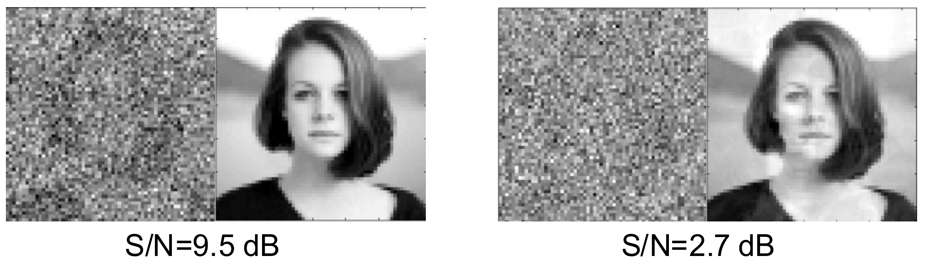
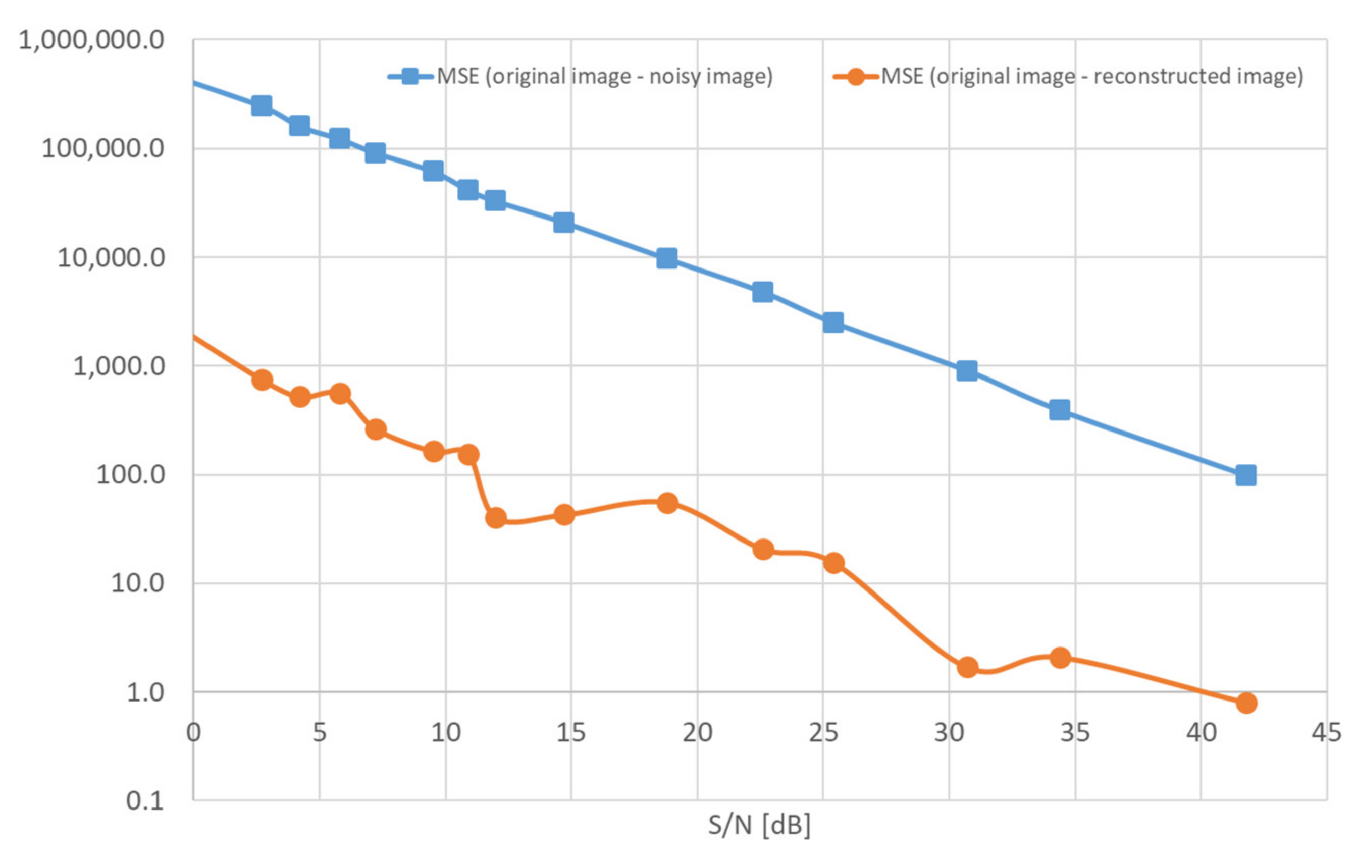
| S/N Ratio [dB] | MSE (Original Image—Noisy Image) | MSE (Original Image—Reconstructed Image) | Index Value |
|---|---|---|---|
| 41.8 | 98.6 | 0.8 | 9.04 |
| 34.4 | 391.9 | 2.1 | 8.97 |
| 30.7 | 909.3 | 1.7 | 9.01 |
| 25.4 | 2523.1 | 15.6 | 8.79 |
| 22.6 | 4807.1 | 20.7 | 8.78 |
| 18.8 | 9698.9 | 55.6 | 9.39 |
| 14.7 | 20,942.0 | 42.9 | 8.54 |
| 12.0 | 32,932.0 | 40.4 | 9.06 |
| 10.9 | 41,500.0 | 155.2 | 9.14 |
| 9.5 | 61,752.0 | 164.5 | 8.66 |
| 7.2 | 91,527.0 | 266.6 | 9.53 |
| 5.8 | 122,950.0 | 563.4 | 8.13 |
| 4.2 | 16,0360.0 | 521.0 | 7.14 |
| 2.7 | 24,6230.0 | 754.2 | 10.45 |
| −2.5 | 62,9540.0 | 4375.8 | 11.17 |
Publisher’s Note: MDPI stays neutral with regard to jurisdictional claims in published maps and institutional affiliations. |
© 2022 by the authors. Licensee MDPI, Basel, Switzerland. This article is an open access article distributed under the terms and conditions of the Creative Commons Attribution (CC BY) license (https://creativecommons.org/licenses/by/4.0/).
Share and Cite
Citko, W.; Sienko, W. Inpainted Image Reconstruction Using an Extended Hopfield Neural Network Based Machine Learning System. Sensors 2022, 22, 813. https://doi.org/10.3390/s22030813
Citko W, Sienko W. Inpainted Image Reconstruction Using an Extended Hopfield Neural Network Based Machine Learning System. Sensors. 2022; 22(3):813. https://doi.org/10.3390/s22030813
Chicago/Turabian StyleCitko, Wieslaw, and Wieslaw Sienko. 2022. "Inpainted Image Reconstruction Using an Extended Hopfield Neural Network Based Machine Learning System" Sensors 22, no. 3: 813. https://doi.org/10.3390/s22030813
APA StyleCitko, W., & Sienko, W. (2022). Inpainted Image Reconstruction Using an Extended Hopfield Neural Network Based Machine Learning System. Sensors, 22(3), 813. https://doi.org/10.3390/s22030813