
Optimizing the Ultrasound Tongue Image Representation for Residual Network-Based Articulatory-to-Acoustic Mapping
 , ,
, ,  and
and 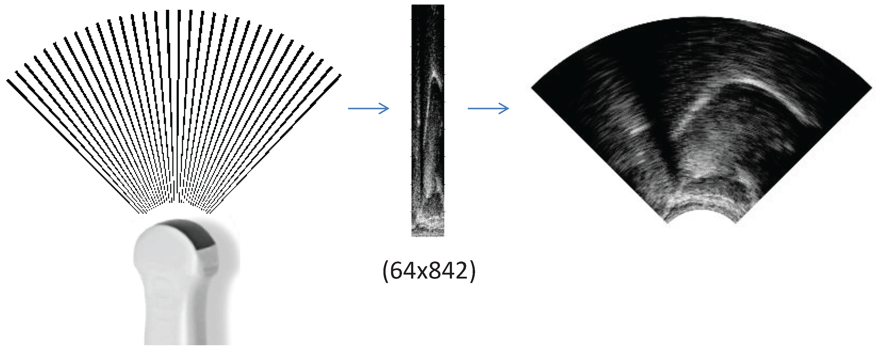
Abstract
1. Introduction
1.1. Representations of Ultrasound Tongue Images
1.2. Contributions of This Paper
2. Materials and Methods
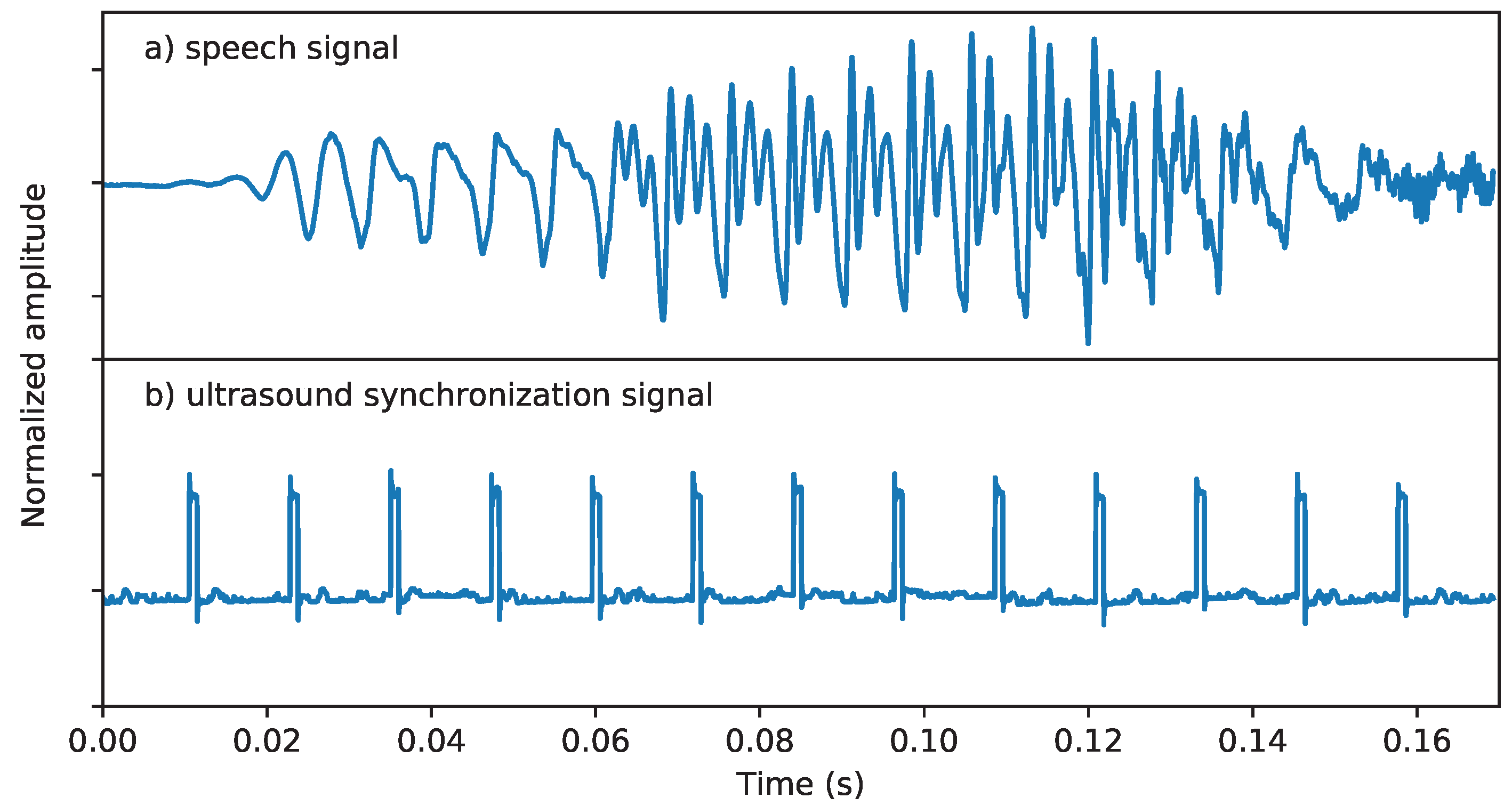
2.1. Data Acquisition
2.2. Input 1: Ultrasound as Raw Scanlines (UTIraw)
2.3. Input 2: Ultrasound as Raw Scanlines, Reshaped to Square (UTIraw-Padding)
2.4. Input 3: Ultrasound as a Wedge-Shape (UTIwedge)
2.5. Target: Spectral Features of the Vocoder
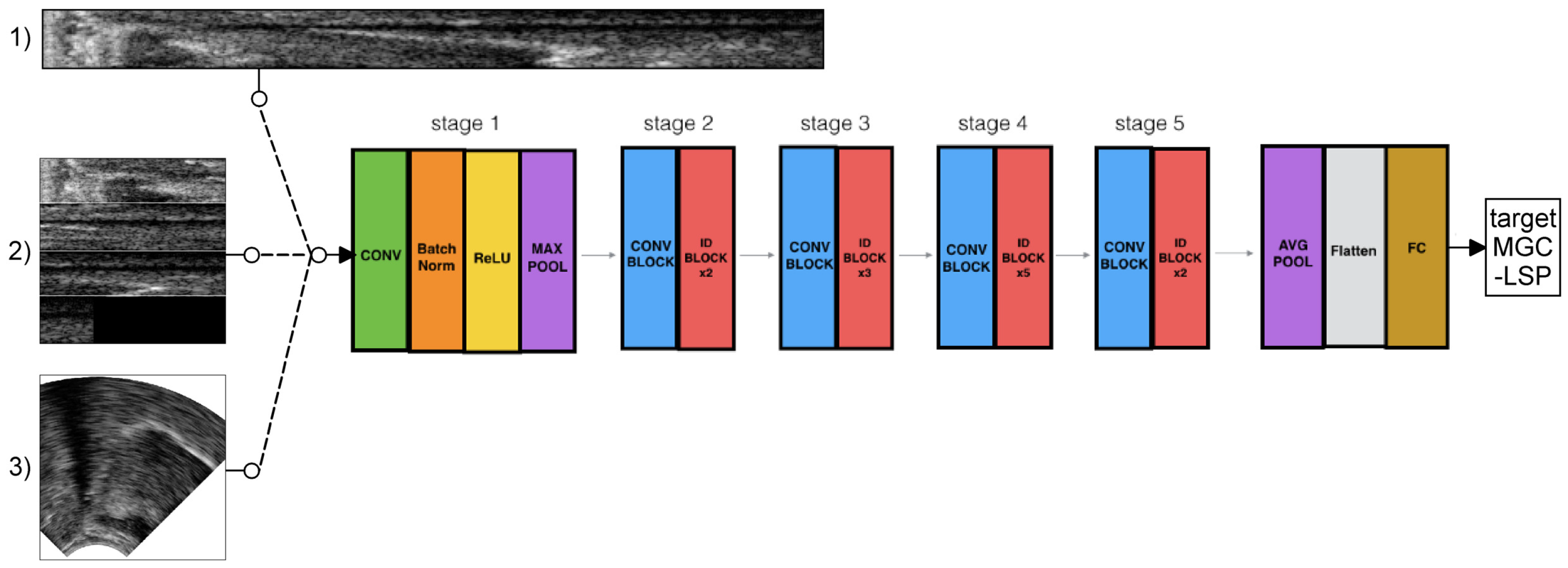
2.6. Training of Deep Neural Networks
3. Results
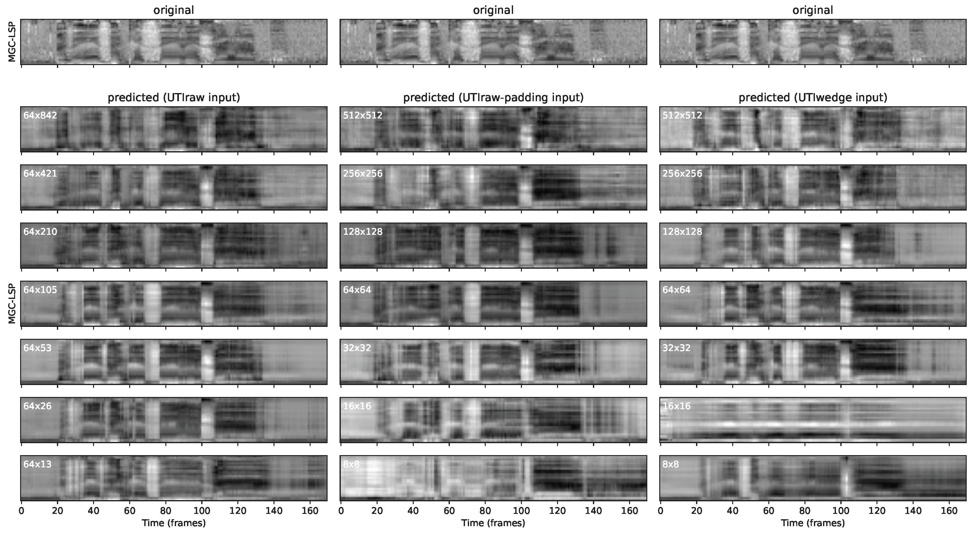
3.1. Demonstration Samples
3.2. Comparison of Raw Scanline Data and Wedge Format
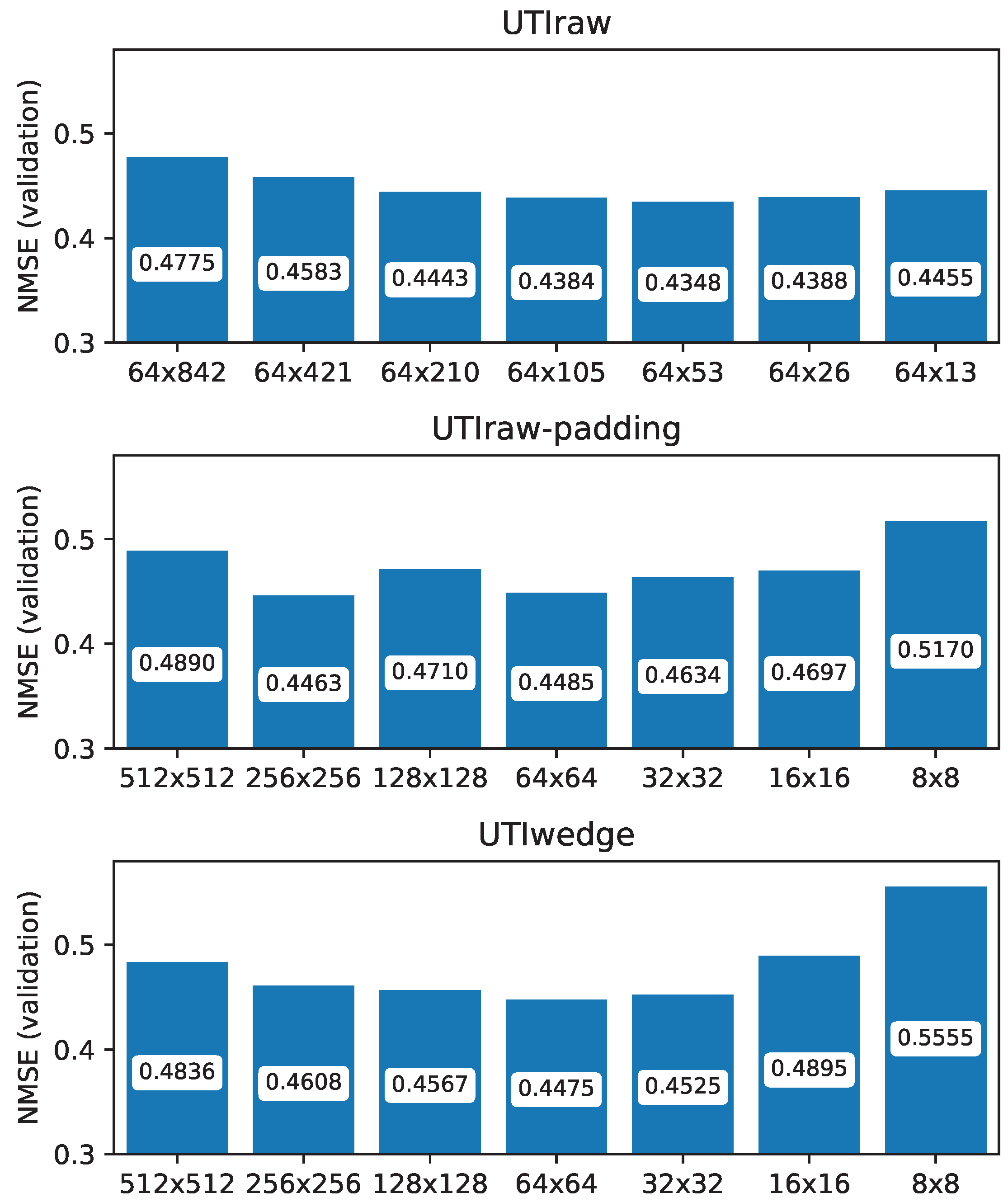
3.3. Relation of Input Image Size and NMSE
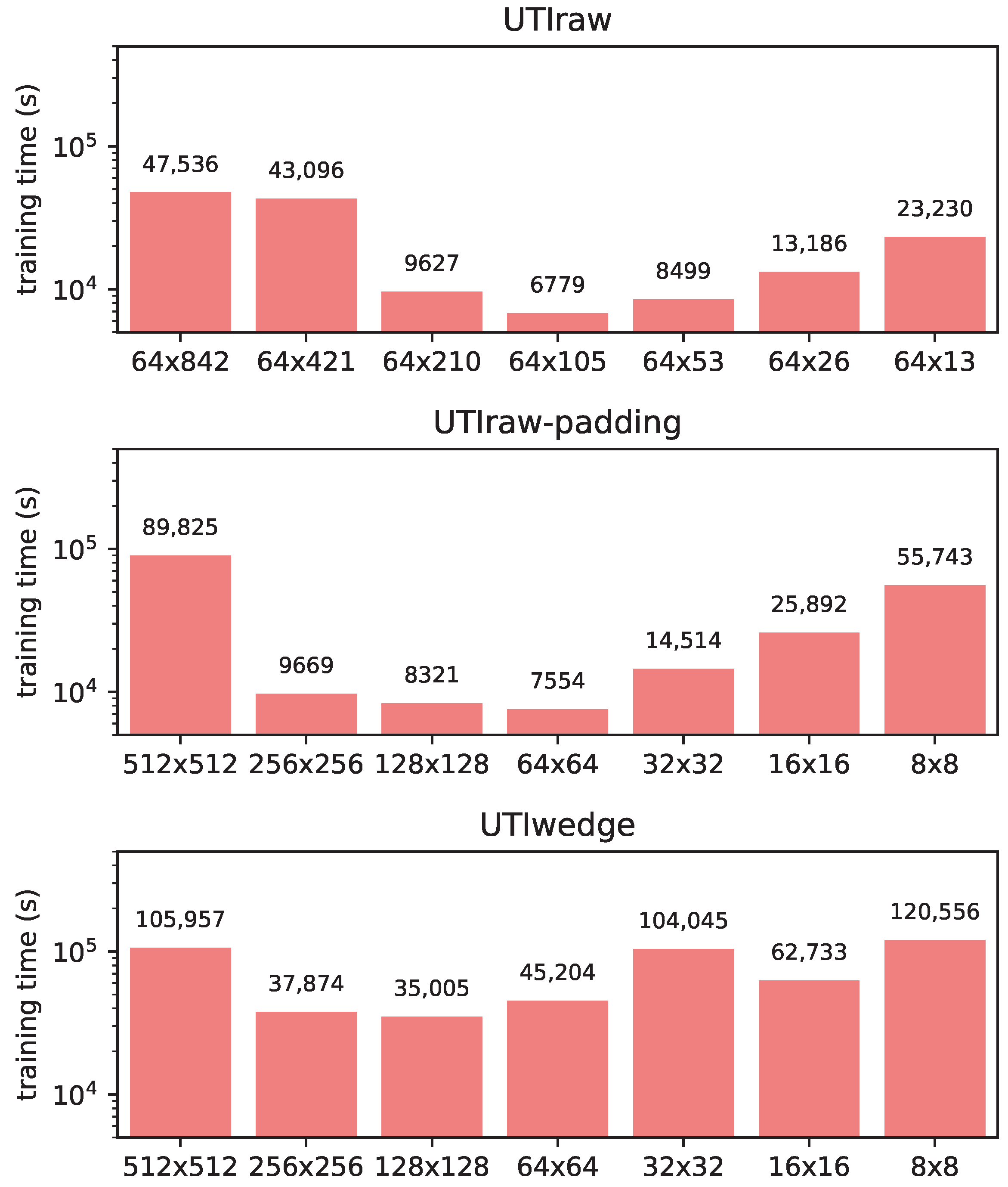
3.4. Training Time
4. Discussion
5. Conclusions
Author Contributions
Funding
Institutional Review Board Statement
Informed Consent Statement
Data Availability Statement
Acknowledgments
Conflicts of Interest
Abbreviations
| AAI | Acoustic-to-Articulatory Inversion |
| AAM | Articulatory-to-Acoustic Mapping |
| CNN | Convolutional Neural Network |
| DNN | Deep Neural Network |
| EMA | Electromagnetic Articulography |
| EOS | Electro-Optical Stomatography |
| LSTM | Long-Short Term Memory |
| MGC-LSP | Mel-Generalized Cepstrum–Line Spectral Pair |
| MGLSA | Mel-Generalized Log Spectral Approximation |
| PMA | Permanent Magnetic Articulography |
| sEMG | surface Electromyography |
| SSI | Silent Speech Interface |
| SSR | Silent Speech Recognition |
| TTS | Text-To-Speech |
| UTI | Ultrasound Tongue Imaging |
References
- Denby, B.; Schultz, T.; Honda, K.; Hueber, T.; Gilbert, J.M.; Brumberg, J.S. Silent speech interfaces. Speech Commun. 2010, 52, 270–287. [Google Scholar] [CrossRef]
- Schultz, T.; Wand, M.; Hueber, T.; Krusienski, D.J.; Herff, C.; Brumberg, J.S. Biosignal-Based Spoken Communication: A Survey. IEEE/ACM Trans. Audio, Speech Lang. Process. 2017, 25, 2257–2271. [Google Scholar] [CrossRef]
- Gonzalez-Lopez, J.A.; Gomez-Alanis, A.; Martin Donas, J.M.; Perez-Cordoba, J.L.; Gomez, A.M. Silent Speech Interfaces for Speech Restoration: A Review. IEEE Access 2020, 8, 177995–178021. [Google Scholar] [CrossRef]
- Denby, B.; Stone, M. Speech synthesis from real time ultrasound images of the tongue. In Proceedings of the ICASSP, Montreal, QC, Canada, 17–21 May 2004; pp. 685–688. [Google Scholar] [CrossRef]
- Denby, B.; Cai, J.; Hueber, T.; Roussel, P.; Dreyfus, G.; Crevier-Buchman, L.; Pillot-Loiseau, C.; Chollet, G.; Manitsaris, S.; Stone, M. Towards a Practical Silent Speech Interface Based on Vocal Tract Imaging. In Proceedings of the 9th International Seminar on Speech Production (ISSP 2011), Montreal, QC, Canada, 20–23 June 2011; pp. 89–94. [Google Scholar]
- Hueber, T.; Benaroya, E.L.; Chollet, G.; Dreyfus, G.; Stone, M. Development of a silent speech interface driven by ultrasound and optical images of the tongue and lips. Speech Commun. 2010, 52, 288–300. [Google Scholar] [CrossRef]
- Hueber, T.; Benaroya, E.l.; Denby, B.; Chollet, G. Statistical Mapping Between Articulatory and Acoustic Data for an Ultrasound-Based Silent Speech Interface. In Proceedings of the Interspeech, Florence, Italy, 27–31 August 2011; pp. 593–596. [Google Scholar]
- Wei, J.; Fang, Q.; Zheng, X.; Lu, W.; He, Y.; Dang, J. Mapping ultrasound-based articulatory images and vowel sounds with a deep neural network framework. Multimed. Tools Appl. 2016, 75, 5223–5245. [Google Scholar] [CrossRef]
- Jaumard-Hakoun, A.; Xu, K.; Leboullenger, C.; Roussel-Ragot, P.; Denby, B. An Articulatory-Based Singing Voice Synthesis Using Tongue and Lips Imaging. In Proceedings of the Interspeech, San Francisco, CA, USA, 8–12 September 2016; pp. 1467–1471. [Google Scholar] [CrossRef]
- Tatulli, E.; Hueber, T. Feature extraction using multimodal convolutional neural networks for visual speech recognition. In Proceedings of the ICASSP, New Orleans, LA, USA, 5–9 March 2017; pp. 2971–2975. [Google Scholar] [CrossRef]
- Csapó, T.G.; Grósz, T.; Gosztolya, G.; Tóth, L.; Markó, A. DNN-Based Ultrasound-to-Speech Conversion for a Silent Speech Interface. In Proceedings of the Interspeech, Stockholm, Sweden, 20–24 August 2017; pp. 3672–3676. [Google Scholar] [CrossRef]
- Grósz, T.; Gosztolya, G.; Tóth, L.; Csapó, T.G.; Markó, A. F0 Estimation for DNN-Based Ultrasound Silent Speech Interfaces. In Proceedings of the ICASSP, Calgary, AB, Canada, 15–20 April 2018; pp. 291–295. [Google Scholar]
- Tóth, L.; Gosztolya, G.; Grósz, T.; Markó, A.; Csapó, T.G. Multi-Task Learning of Phonetic Labels and Speech Synthesis Parameters for Ultrasound-Based Silent Speech Interfaces. In Proceedings of the Interspeech, Hyderabad, India, 2–6 September 2018; pp. 3172–3176. [Google Scholar] [CrossRef]
- Ji, Y.; Liu, L.; Wang, H.; Liu, Z.; Niu, Z.; Denby, B. Updating the Silent Speech Challenge benchmark with deep learning. Speech Commun. 2018, 98, 42–50. [Google Scholar] [CrossRef]
- Moliner, E.; Csapó, T.G. Ultrasound-based silent speech interface using convolutional and recurrent neural networks. Acta Acust. United Acust. 2019, 105, 587–590. [Google Scholar] [CrossRef]
- Gosztolya, G.; Pintér, Á.; Tóth, L.; Grósz, T.; Markó, A.; Csapó, T.G. Autoencoder-Based Articulatory-to-Acoustic Mapping for Ultrasound Silent Speech Interfaces. In Proceedings of the International Joint Conference on Neural Networks, Budapest, Hungary, 14–19 July 2019. [Google Scholar]
- Csapó, T.G.; Al-Radhi, M.S.; Németh, G.; Gosztolya, G.; Grósz, T.; Tóth, L.; Markó, A. Ultrasound-based Silent Speech Interface Built on a Continuous Vocoder. In Proceedings of the Interspeech, Graz, Austria, 15–19 September 2019; pp. 894–898. [Google Scholar] [CrossRef]
- Kimura, N.; Kono, M.C.; Rekimoto, J. Sottovoce: An ultrasound imaging-based silent speech interaction using deep neural networks. In Proceedings of the CHI’19: 2019 CHI Conference on Human Factors in Computing Systems, Glasgow, UK, 4–9 May 2019; pp. 1–11. [Google Scholar] [CrossRef]
- Zhang, J.; Roussel, P.; Denby, B. Creating Song from Lip and Tongue Videos with a Convolutional Vocoder. IEEE Access 2021, 9, 13076–13082. [Google Scholar] [CrossRef]
- Csapó, T.G.; Zainkó, C.; Tóth, L.; Gosztolya, G.; Markó, A. Ultrasound-based Articulatory-to-Acoustic Mapping with WaveGlow Speech Synthesis. In Proceedings of the Interspeech, Shanghai, China, 25–29 October 2020; pp. 2727–2731. [Google Scholar] [CrossRef]
- Shandiz, A.H.; Tóth, L.; Gosztolya, G.; Markó, A.; Csapó, T.G. Neural speaker embeddings for ultrasound-based silent speech interfaces. In Proceedings of the Interspeech, Brno, Czech Republic, 30 August–3 September 2021; pp. 151–155. [Google Scholar] [CrossRef]
- Shandiz, A.H.; Tóth, L.; Gosztolya, G.; Markó, A.; Csapó, T.G. Improving Neural Silent Speech Interface Models by Adversarial Training. In Proceedings of the 2nd International Conference on Artificial Intelligence and Computer Vision (AICV2021), Settat, Morocco, 28–30 June 2021. [Google Scholar]
- Wang, J.; Samal, A.; Green, J.R.; Rudzicz, F. Sentence Recognition from Articulatory Movements for Silent Speech Interfaces. In Proceedings of the ICASSP, Kyoto, Japan, 25–30 March 2012; pp. 4985–4988. [Google Scholar]
- Kim, M.; Cao, B.; Mau, T.; Wang, J. Speaker-Independent Silent Speech Recognition from Flesh-Point Articulatory Movements Using an LSTM Neural Network. IEEE/ACM Trans. Audio Speech Lang. Process. 2017, 25, 2323–2336. [Google Scholar] [CrossRef] [PubMed]
- Cao, B.; Kim, M.; Wang, J.R.; Van Santen, J.; Mau, T.; Wang, J. Articulation-to-Speech Synthesis Using Articulatory Flesh Point Sensors’ Orientation Information. In Proceedings of the Interspeech, Hyderabad, India, 2–6 September 2018; pp. 3152–3156. [Google Scholar] [CrossRef]
- Taguchi, F.; Kaburagi, T. Articulatory-to-speech conversion using bi-directional long short-term memory. In Proceedings of the Interspeech, Hyderabad, India, 2–6 September 2018; pp. 2499–2503. [Google Scholar]
- Cao, B.; Wisler, A.; Wang, J. Speaker Adaptation on Articulation and Acoustics for Articulation-to-Speech Synthesis. Sensors 2022, 22, 6056. [Google Scholar] [CrossRef] [PubMed]
- Fagan, M.J.; Ell, S.R.; Gilbert, J.M.; Sarrazin, E.; Chapman, P.M. Development of a (silent) speech recognition system for patients following laryngectomy. Med. Eng. Phys. 2008, 30, 419–425. [Google Scholar] [CrossRef] [PubMed]
- Gonzalez, J.A.; Cheah, L.A.; Gomez, A.M.; Green, P.D.; Gilbert, J.M.; Ell, S.R.; Moore, R.K.; Holdsworth, E. Direct Speech Reconstruction from Articulatory Sensor Data by Machine Learning. IEEE/ACM Trans. Audio Speech Lang. Process. 2017, 25, 2362–2374. [Google Scholar] [CrossRef]
- Diener, L.; Janke, M.; Schultz, T. Direct conversion from facial myoelectric signals to speech using Deep Neural Networks. In Proceedings of the 2015 International Joint Conference on Neural Networks (IJCNN), Killarney, Ireland, 12–17 July 2015; IEEE: Piscataway, NJ, USA, 2015; pp. 1–7. [Google Scholar] [CrossRef]
- Janke, M.; Diener, L. EMG-to-Speech: Direct Generation of Speech from Facial Electromyographic Signals. IEEE/ACM Trans. Audio Speech Lang. Process. 2017, 25, 2375–2385. [Google Scholar] [CrossRef]
- Wand, M.; Schultz, T.; Schmidhuber, J. Domain-Adversarial Training for Session Independent EMG-based Speech Recognition. In Proceedings of the Interspeech, Hyderabad, India, 2–6 September 2018; pp. 3167–3171. [Google Scholar] [CrossRef]
- Stone, S.; Birkholz, P. Silent-speech command word recognition using electro-optical stomatography. In Proceedings of the Interspeech, San Francisco, CA, USA, 8–12 September 2016; pp. 2350–2351. [Google Scholar]
- Wand, M.; Koutník, J.; Schmidhuber, J. Lipreading with long short-term memory. In Proceedings of the ICASSP, Shanghai, China, 20–25 March 2016; pp. 6115–6119. [Google Scholar]
- Ephrat, A.; Peleg, S. Vid2speech: Speech Reconstruction from Silent Video. In Proceedings of the ICASSP, New Orleans, LA, USA, 5–9 March 2017; pp. 5095–5099. [Google Scholar]
- Sun, K.; Yu, C.; Shi, W.; Liu, L.; Shi, Y. Lip-Interact: Improving Mobile Device Interaction with Silent Speech Commands. In Proceedings of the UIST 2018—31st Annual ACM Symposium on User Interface Software and Technology, Berlin, Germany, 14–17 October 2018; pp. 581–593. [Google Scholar] [CrossRef]
- Ferreira, D.; Silva, S.; Curado, F.; Teixeira, A. Exploring Silent Speech Interfaces Based on Frequency-Modulated Continuous-Wave Radar. Sensors 2022, 22, 649. [Google Scholar] [CrossRef] [PubMed]
- Freitas, J.; Ferreira, A.J.; Figueiredo, M.A.T.; Teixeira, A.J.S.; Dias, M.S. Enhancing multimodal silent speech interfaces with feature selection. In Proceedings of the Interspeech, Singapore, 14–18 September 2014; pp. 1169–1173. [Google Scholar]
- Stone, M. A guide to analysing tongue motion from ultrasound images. Clin. Linguist. Phon. 2005, 19, 455–501. [Google Scholar] [CrossRef] [PubMed]
- Csapó, T.G.; Lulich, S.M. Error analysis of extracted tongue contours from 2D ultrasound images. In Proceedings of the Interspeech, Dresden, Germany, 6–10 September 2015; pp. 2157–2161. [Google Scholar]
- Wrench, A.; Balch-Tomes, J. Beyond the Edge: Markerless Pose Estimation of Speech Articulators from Ultrasound and Camera Images Using DeepLabCut. Sensors 2022, 22, 1133. [Google Scholar] [CrossRef] [PubMed]
- Hueber, T.; Aversano, G.; Chollet, G.; Denby, B.; Dreyfus, G.; Oussar, Y.; Roussel, P.; Stone, M. Eigentongue feature extraction for an ultrasound-based silent speech interface. In Proceedings of the ICASSP, Honolulu, HI, USA, 15–20 April 2007; pp. 1245–1248. [Google Scholar]
- Kimura, N.; Su, Z.; Saeki, T.; Rekimoto, J. SSR7000: A Synchronized Corpus of Ultrasound Tongue Imaging for End-to-End Silent Speech Recognition. In Proceedings of the Language Resources and Evaluation Conference, Marseille, France, 20–25 June 2022; pp. 6866–6873. [Google Scholar]
- Yu, Y.; Honarmandi Shandiz, A.; Tóth, L. Reconstructing Speech from Real-Time Articulatory MRI Using Neural Vocoders. In Proceedings of the EUSIPCO, Dublin, Ireland, 23–27 August 2021; pp. 945–949. [Google Scholar]
- Ribeiro, M.S.; Eshky, A.; Richmond, K.; Renals, S. Speaker-independent Classification of Phonetic Segments from Raw Ultrasound in Child Speech. In Proceedings of the ICASSP, Brighton, UK, 12–17 May 2019; pp. 1328–1332. [Google Scholar] [CrossRef]
- Ribeiro, M.S.; Eshky, A.; Richmond, K.; Renals, S. Silent versus modal multi-speaker speech recognition from ultrasound and video. In Proceedings of the Interspeech, Brno, Czech Republic, 30 August–3 September 2021; pp. 641–645. [Google Scholar]
- Imai, S.; Sumita, K.; Furuichi, C. Mel Log Spectrum Approximation (MLSA) filter for speech synthesis. Electron. Commun. Jpn. Part I Commun. 1983, 66, 10–18. [Google Scholar] [CrossRef]
- Tokuda, K.; Kobayashi, T.; Masuko, T.; Imai, S. Mel-generalized cepstral analysis—A unified approach to speech spectral estimation. In Proceedings of the ICSLP, Yokohama, Japan, 18–22 September 1994; pp. 1043–1046. [Google Scholar]
- He, K.; Zhang, X.; Ren, S.; Sun, J. Deep Residual Learning for Image Recognition. In Proceedings of the 2016 IEEE Conference on Computer Vision and Pattern Recognition (CVPR), Las Vegas, NV, USA, 27–30 June 2016; pp. 770–778. [Google Scholar] [CrossRef]
- Csapó, T.G.; Deme, A.; Gráczi, T.E.; Markó, A.; Varjasi, G. Synchronized speech, tongue ultrasound and lip movement video recordings with the “Micro” system. In Proceedings of the Challenges in Analysis and Processing of Spontaneous Speech, Budapest, Hungary, 14–17 May 2017. [Google Scholar]
- Eshky, A.; Ribeiro, M.S.; Cleland, J.; Richmond, K.; Roxburgh, Z.; Scobbie, J.M.; Wrench, A. UltraSuite: A Repository of Ultrasound and Acoustic Data from Child Speech Therapy Sessions. In Proceedings of the Interspeech, Hyderabad, India, 2–6 September 2018; ISCA: Hyderabad, India, 2018; pp. 1888–1892. [Google Scholar] [CrossRef]
- Ribeiro, M.S.; Sanger, J.; Zhang, J.X.X.; Eshky, A.; Wrench, A.; Richmond, K.; Renals, S. TaL: A synchronised multi-speaker corpus of ultrasound tongue imaging, audio, and lip videos. In Proceedings of the 2021 IEEE Spoken Language Technology Workshop (SLT), Online, 19–22 January 2021; pp. 1109–1116. [Google Scholar] [CrossRef]
- Czap, L. Impact of preprocessing features on the performance of ultrasound tongue contour tracking, via dynamic programming. Acta Polytech. Hung. 2021, 18, 159–176. [Google Scholar] [CrossRef]
- Lulich, S.M.; Berkson, K.H.; de Jong, K. Acquiring and visualizing 3D/4D ultrasound recordings of tongue motion. J. Phon. 2018, 71, 410–424. [Google Scholar] [CrossRef]
- Czap, L. A Nyelvkontúr Automatikus Követése és Elemzése Ultrahang Felvételeken [Automatic Tracking and Analysis of the Tongue Contour on Ultrasound Recordings]. Habilitation Thesis, University of Miskolc, Miskolc, Hungary, 2020. [Google Scholar]
- Maier-Hein, L.; Metze, F.; Schultz, T.; Waibel, A. Session independent non-audible speech recognition using surface electromyography. In Proceedings of the ASRU, San Juan, Puerto Rico, 27 November–1 December 2005; IEEE: San Juan, Puerto Rico, 2005; pp. 331–336. [Google Scholar] [CrossRef]
- Janke, M.; Wand, M.; Nakamura, K.; Schultz, T. Further investigations on EMG-to-speech conversion. In Proceedings of the ICASSP, Kyoto, Japan, 25–30 March 2012; IEEE: Kyoto, Japan, 2012; pp. 365–368. [Google Scholar] [CrossRef]
- Stone, S.; Birkholz, P. Cross-speaker silent-speech command word recognition using electro-optical stomatography. In Proceedings of the ICASSP, Barcelona, Spain, 4–8 May 2020; pp. 7849–7853. [Google Scholar]
- Csapó, T.G.; Xu, K. Quantification of Transducer Misalignment in Ultrasound Tongue Imaging. In Proceedings of the Interspeech, Shanghai, China, 25–29 October 2020; pp. 3735–3739. [Google Scholar] [CrossRef]
- Csapó, T.G.; Xu, K.; Deme, A.; Gráczi, T.E.; Markó, A. Transducer Misalignment in Ultrasound Tongue Imaging. In Proceedings of the 12th International Seminar on Speech Production, New Haven, CT, USA, 14–18 December 2020. [Google Scholar]


Publisher’s Note: MDPI stays neutral with regard to jurisdictional claims in published maps and institutional affiliations. |
© 2022 by the authors. Licensee MDPI, Basel, Switzerland. This article is an open access article distributed under the terms and conditions of the Creative Commons Attribution (CC BY) license (https://creativecommons.org/licenses/by/4.0/).
Share and Cite
Csapó, T.G.; Gosztolya, G.; Tóth, L.; Shandiz, A.H.; Markó, A. Optimizing the Ultrasound Tongue Image Representation for Residual Network-Based Articulatory-to-Acoustic Mapping. Sensors 2022, 22, 8601. https://doi.org/10.3390/s22228601
Csapó TG, Gosztolya G, Tóth L, Shandiz AH, Markó A. Optimizing the Ultrasound Tongue Image Representation for Residual Network-Based Articulatory-to-Acoustic Mapping. Sensors. 2022; 22(22):8601. https://doi.org/10.3390/s22228601
Chicago/Turabian StyleCsapó, Tamás Gábor, Gábor Gosztolya, László Tóth, Amin Honarmandi Shandiz, and Alexandra Markó. 2022. "Optimizing the Ultrasound Tongue Image Representation for Residual Network-Based Articulatory-to-Acoustic Mapping" Sensors 22, no. 22: 8601. https://doi.org/10.3390/s22228601
APA StyleCsapó, T. G., Gosztolya, G., Tóth, L., Shandiz, A. H., & Markó, A. (2022). Optimizing the Ultrasound Tongue Image Representation for Residual Network-Based Articulatory-to-Acoustic Mapping. Sensors, 22(22), 8601. https://doi.org/10.3390/s22228601