1. Introduction
The optical transport network (OTN) is a transport network that enables the transmission, multiplexing, route selection, and monitoring of service signals in an optical domain, ensuring its performance index and survivability. The OTN can support the transparent transmission of customer signals, high-bandwidth multiplexing, and configuration. It also provides end-to-end connectivity and networking capabilities. With the rapid development of network communication technology, the demand for OTN networks has increased significantly in terms of the scale of information volume, demand complexity, and dynamic spatio-temporal distribution. Unlike traditional networks, the OTN can meet more network requirements due to its suitable transmission medium, which has a high transmission speed, more data transmission, and a long transmission distance.
Traditional routing design schemes manually model network demand characteristics and design routing policies in a focused way. The traditional routing protocol is designed for wired networks, with a fixed bandwidth allocation pattern and low bandwidth utilization. It cannot provide differentiated services based on the level of assistance, nor can it cope with the rapid changes in topology and link quality standards in optical network environments. Additionally, because OTN demand has complex spatio-temporal distribution fluctuations, the optimization problem of its routing is an NP-hard problem [
1]. In this case, traditional network routing design schemes do not apply to the OTN.
With the development of new network architectures, such as the software-defined networking (SDN) and the maturation of deep reinforcement learning (DRL) techniques in recent years, software-defined optical transport networks (SD-OTNs) based on the SDN are gaining popularity in the industry. Recent studies have used the DRL to address SDN-related problems, such as QoS-aware secure routing for the SDN-IoT [
2], SDN routing optimization problems [
3], and the SDN demand control [
4]. However, due to DRL agents’ lack of generalization capabilities, they do not achieve good results in new network topologies. Thus, DRL agents cannot make correct routing decisions when presented with unexplored network scenarios during the training phase. The main reason behind this phenomenon is that graphs essentially represent computer networks. In addition, traditional DRL algorithms use typical neural network (NN) architectures (e.g., fully connected convolutional neural networks), which are unsuitable for modeling information about graph structures. Due to the computational effort and high time complexity of the routing optimization problem, traditional DRL algorithms are challenging for the DRL agent to converge quickly when addressing the network routing optimization problem. Additionally, OTN network problems are incredibly complex and have high trial-and-error costs, making it difficult to implement DRL algorithms in real optical networks.
This paper proposes an ensembles- and message-passing neural-network-based deep Q-network (EMDQN) method to solve the SD-OTN routing decision problem. The message-passing neural network (MPNN) is a deep learning (DL) method based on a graph structure [
5]. The MPNN contributes to learning the relationship between graph elements and their rules. In this paper, the MPNN is used to capture information about the relationship between the demand on links and network topology, which can improve the model’s generalization ability. Despite computationally complex network problems, ensemble learning has a unique advantage that can increase sample utilization. We reweigh the sample transitions based on the uncertainty estimates of ensemble learning. This method can improve the signal-to-noise ratio during Q-network updates, and stabilize the learning process of the EMDQN agent, which helps the deep Q-network (DQN) [
6] operate stably in OTN networks.
The main contributions of this paper are as follows:
We propose an SD-OTN routing optimization algorithm based on the reinforcement learning model of the EMDQN. To effectively improve the extrapolation capability of DRL decision-makers, we design a more refined state representation and a limited set of actions.
We use the MPNN algorithm instead of the traditional DQN’s policy networks, which can capture the relationship between links and network topology demand and improve the DRL decision-maker performance and generalization capability. Additionally, we exploit the advantages of efficient exploration through ensemble learning to explore the environment in parallel and improve convergence performance.
We design practical comparison experiments to verify the superior performance of the EMDQN model.
The rest of this paper is structured as follows. In
Section 2, this paper discusses research related to the proposed solution for the network problem.
Section 3 describes the software-defined network system architecture and the OTN optimization scenarios and tasks. In
Section 4, this paper describes the design of DRL-based routing optimization decisions. In
Section 5, this paper presents an extensive evaluation of DRL-based solutions in some realistic OTN scenarios. Finally, in
Section 6, we present our conclusion and directions for future work.
2. Related Research
Traditional routing optimization schemes are usually based on the OSPF (open shortest path first) [
7] or ECMP (equal-cost multipath routing) [
8]. The OSPF protocol routes all flow requests individually to the shortest path. The ECMP protocol increases transmission bandwidth using multiple links simultaneously. However, these approaches, based on fixed forwarding rules, are prone to link congestion and cannot meet the demand of exponential traffic growth. Recently, most heuristic algorithm-based approaches have been built under the architecture of the SDN. The authors in [
9] proposed a heuristic ant-colony-based dynamic layout algorithm for SDNs with multiple controllers, which can effectively reduce controller-to-switch and controller-to-controller communication delays caused by link failures. The authors in [
10] applied a random-based heuristic method called the alienated ant algorithm, which forces ants to spread out across all available paths while searching for food rather than converging on a single path. The authors in [
11] analytically extract historical user data through a semi-supervised clustering algorithm for efficient data classification, analysis, and feature extraction. Subsequently, they used a supervised classification algorithm to predict the flow of service demand. The authors in [
12] proposed a heuristic algorithm-based solution for DWDM-based OTN network planning. The authors in [
13] proposed a least-cost tree heuristic algorithm to solve the OTN path-sharing and load-balancing problem. However, because of a lack of historical experience in data learning, heuristic algorithms can only build models for specific problems. When the network changes, it is difficult to determine the network parameters and there is limited scalability to guarantee service quality. Furthermore, because of the tremendous computational effort and high computational complexity of these methods, heuristic algorithms do not perform well on OTN networks.
With SDN’s maturity and large-scale commercialization, the SD-OTN based on the SDN is becoming increasingly popular in the industry. SD-OTN adapts the reconfigurable optical add-drop multiplexer (ROADM) nodes through the southbound interface protocol and establishes a unified resource and service model. The SD-OTN controller can realize topology and network status data collection, routing policy distribution, and network monitoring. Therefore, many researchers deploy artificial intelligence algorithms in the controller. Deep learning, with its powerful learning algorithms and excellent performance advantages, has gradually been applied to the SDN. To solve the SDN load-balancing problem, Chen et al. [
14] used the long short-term memory (LSTM) to predict the network traffic in the SDN application plane. The authors in [
15] proposed a weighted Markov prediction model based on mobile user classification to optimize network resources and reduce network congestion. The authors in [
16] proposed an intrusion detection system based on SDN and deep learning, reducing the burden of security configuration files on network devices. However, deep learning requires many datasets for training and has poor generalization abilities due to its inability to interact with the environment. These factors make it difficult to optimize the performance of dynamic networks. Compared with deep learning, reinforcement learning uses online learning for model training, changing agent behaviors through continuous exploration, learning, and experimentation to obtain the best return. Therefore, reinforcement learning does not require the model to be trained in advance. It can change its action according to the environment and reward feedback. The authors in [
17] designed a Q-learning-based localization-free routing for underwater sensor networks. The authors in [
18] proposed a deep Q-routing algorithm to compute the path of any source-destination pair request using a deep Q-network with prioritized experience replay. The authors in [
19] proposed traction control ideas to solve the routing problem. The authors in [
20] proposed a routing optimization algorithm based on the proximal policy optimization (PPO) model in reinforcement learning. The authors in [
21] discussed a solution for automatic routing in the OTN using DRL. Although the studies described above have been successful for the SDN demand-routing optimization problem, they do not perform as well in new topologies because they do not consider the model’s generalization capability.
The traditional DRL algorithms use a typical neural network (NN) as the policy network. The NN can extract and filter the features of the input information and data layer by layer to finally obtain the results of tasks, such as classification and prediction. However, as research advances, conventional neural networks are unable to solve all network routing problems and will struggle to handle non-Euclidean-structured graph data. Therefore, we need to optimize the traditional reinforcement learning algorithm to improve its ability to extract the information features of the sample. Off-policy reinforcement learning (Off-policy RL) algorithms significantly improve sample utilization by reusing past experiences. The authors in [
22] propose an off-policy actor–critic RL algorithm based on a maximum entropy reinforcement learning framework. The participants’ goal in this framework is to maximize the expected reward while maximizing the entropy. They achieved state-of-the-art sample efficiency results by combining a maximum entropy framework. However, in practice, the commonly used off-policy approximate dynamic programming methods based on the Q-learning and actor–critic methods are susceptible to data distribution. They can only make limited progress without collecting additional on-policy data. To address this problem, the authors in [
23] proposed bootstrap error accumulation reduction to reduce off-policy algorithm instability caused by accumulating backup operators via the Bellman algorithm. The authors in [
24] developed a new estimator called offline dual reinforcement learning, which is based on the cross-folding estimation of Q-functions and marginalized density ratios. The authors in [
25] used a framework combining imitation learning and deep reinforcement learning, effectively reducing the RL algorithm’s instability. The authors in [
26] used the DQN replay datasets to study off-policy RL, effectively reducing the off-policy algorithm’s instability. The authors in [
27] proposed an intelligent routing algorithm combining the graph neural network (GNN) and deep deterministic policy gradient (DDPG) in the SDN environment, which can be effectively extended to different network topologies, improving load-balancing capabilities and generalizability. The authors in [
28] combined GNN with the DQN algorithm to address the lack of generalization abilities in untrained OTN topologies. OTN topology graphs are non-Euclidean data, and the nodes in their topology graphs typically contain useful feature information that most neural networks are unable to comprehend. They use MPNN to extract feature information between OTN topological nodes, which improves the generalization performance of the DRL algorithm.
However, it is a challenge for a single DRL agent to balance exploration and development, resulting in limited convergence performance. Ensemble learning solves a single prediction problem by building several models. It works by generating several classifiers or models, each of which learns and predicts independently. These predictions are finally combined into a combined prediction, which outperforms any single classification for making predictions [
29]. There are two types of integrated base learning machines. One type involves using various learning algorithms on the same dataset to obtain a base learning machine, which is usually referred to as heterogeneous [
30,
31,
32]. The other type applies the same learning algorithm on a different training set (which can be obtained by random sampling based on the original training dataset, etc.), and the base learning machine obtained using this method is said to be a homogeneous type. However, because of the high implementation difficulty and low scalability of heterogeneous types of base learning machines, expansion to high-dimensional state and action spaces is difficult, making it unsuitable for solving OTN routing optimization problems.
Table 1 summarizes the description of the papers reviewed, whether SDN and RL are considered, and the evaluation indicators. The EMDQN algorithm we propose applies the same reinforcement learning algorithm to different training sets to generate the base learning machine. We combine multiple EMDQN agents to construct an ensemble learning machine and generate diverse samples to effectively generate learning machines with high generalization abilities and significant differences.
4. EMDQN-Based Decision Design for Routing Optimization
In this section, we describe in detail the EMDQN algorithm proposed in this paper.
4.1. DRL-Based Routing Optimization in SD-OTN
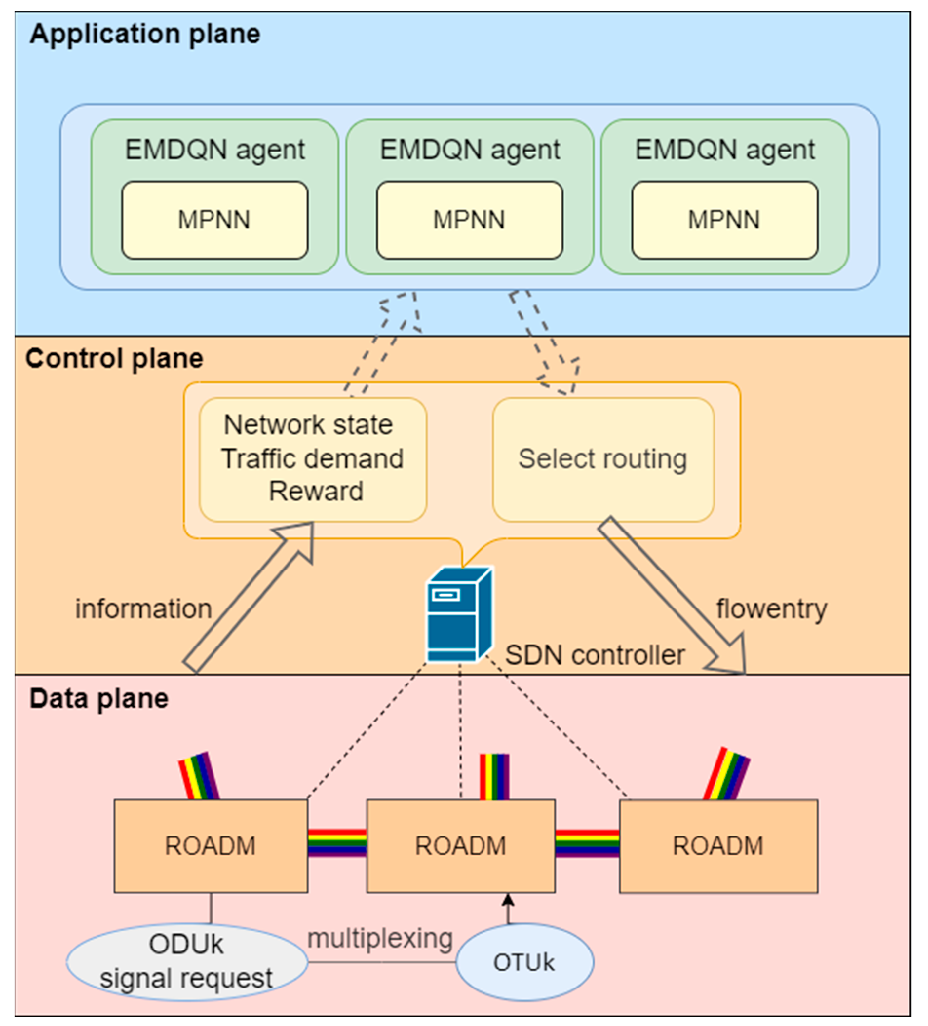
Based on the system architecture described above, the DRL agent’s role is to assign routes to incoming traffic demands for a specific sequence of optical paths (i.e., end-to-end paths) to maximize network utility. Because the DRL agent operates in the electrical domain, traffic demands are treated as requests for ODU signals. These signals, which may originate from different clients, are multiplexed into an optical transform unit (OTU), as shown in
Figure 1. The final OTU frames are transmitted through the optical channels in the OTN [
33].
We use
to refer to an optical transmission network, as shown in Equation (1):
where
and
represent the set of
ROADM nodes and
optical links in the network topology, respectively, as shown in Equations (2) and (3).
We use
to denote the set of link bandwidth capacity, as shown in Equation (4), where
:
The path
from node
to node
is defined as a sequence of links, as shown in Equation (5), where
:
We use
to denote the traffic demand of the path
, and define
as the set of all traffic demands, as shown in Equation (6):
The traffic routing problem in OTN is a classical resource allocation problem [
26]. If the bandwidth capacity of the distributed routing path is greater than the size of the bandwidth requirement, the allocation is successful. After successfully allocating bandwidth capacity for a node pair’s traffic demand, the routing path will not be able to release the bandwidth occupied by that demand until the end of this episode. We use
to describe the remaining bandwidth of the link
, which is the link bandwidth capacity
minus the traffic demands of all paths passing through link
, as shown in Equation (7).
is the set of the remaining bandwidth of all links, as shown in Equation (8).
We use
to denote the allocating traffic demand of the path
, as shown in Equation (9).
is the set of all allocating traffic demands, as shown in Equation (10).
The optimization objective in this paper is to successfully allocate as much of the traffic demand as possible, as shown in Equation (11):
In view of the above optimization objective, the routing optimization can be modeled as a Markov decision process, defined by the tuple, where is the state space, is the action space, is the set of transfer probabilities, and is the set of rewards. The specific design is as follows:
Action space: The action space is designed as shortest hop-based paths of source-destination nodes. The action selects one of the paths to transmit the traffic demand of source–destination nodes. The parameter k is customizable and varies according to the topology’s complexity. The action space is invariant to the arrangement of nodes and edges, which is discretely distributed, allowing the DRL agent to understand the actions on arbitrary network states easily.
State space: The state space is designed as the remaining bandwidth
, the traffic demand
, and the link betweenness. The link betweenness is a centrality metric, which indicates how many paths are likely to cross the link. For each node pair in the topology,
candidate shortest routes are calculated, with the link betweenness value being the number of shortest routes passing through the link divided by the total number of paths, as shown in Equation (12), where
represents the betweenness of the link
,
represents he total number of paths,
represents the number of shortest routes passing through the link
in
candidate shortest routes:
Reward function: The reward function returns a positive reward if the selected link has sufficient capacity to support the traffic demand in an episode; otherwise, it returns no reward and terminates the episode. According to the optimization objective in Equation (11), the final reward for the episode is the sum of the rewards of all successfully assigned traffic demand tuples , as shown in Equation (13), where is the number of traffic demand tuples, represents the reward after the action at time , represents the -th traffic demand successfully assigned, and represents the maximum traffic demand successfully assigned. The higher the reward, the more bandwidth demands are successfully allocated in that time step, and the better the network load-balancing capability.
.
4.2. DQN Algorithm
Based on the above DRL-based optimization solution, this paper selects the DQN algorithm to implement a reinforcement learning agent. The DQN is a classical DRL algorithm based on value functions. It combines a convolutional neural network (CNN) with the Q-learning algorithm, using the CNN model to output the Q-value corresponding to each action to ascertain which to perform [
6].
The DQN algorithm uses two network models containing CNNs for learning: the prediction network and the target network, where and are the network parameters of the prediction and target networks, respectively. The prediction network outputs the predicted Q-value corresponding to the action, whereas the target network calculates the target value and updates the parameters of the prediction network based on a loss function. The DQN copies the parameters of the prediction network model to the target network after each C-round iteration.
The prediction network approximates the action value function through the CNN model
, as shown in Equation (14):
The DQN agent selects and executes an action based on an
-greedy policy. The policy generates a random number in
interval through a uniform distribution. If the number is less than
, it selects an action that maximizes the Q-value; otherwise, it selects an action randomly, as shown in Equation (15):
The target network calculates the target value
by obtaining a random mini-batch storage sample from the replay buffer, as shown in Equation (16), where
is the reward value and
is the discount factor:
The DQN defines the loss function of the network using the mean-square error, as shown in Equation (17). The parameter
is updated by the mini-batch semi-gradient descent, as shown in Equations (18) and (19):
where
represents the number of samples and
represents the update parameter.
The target network is used by the DQN to keep the target Q-value constant over time, which reduces the correlation between the predicted and target Q-values to a certain extent. This operation reduces the possibility of loss value oscillation and divergence during training and improves the algorithm’s stability.
4.3. Message-Passing Neural Network
The CNN model has better results in extracting features from Euclidean spatial data (e.g., picture data), characterized by a stable structure and dimensionality. However, graph-structured or topologically structured data are infinitely dimensional and irregular, and the network surrounding each node may be unique. Such structured data renders traditional CNNs ineffective and unable to extract data features effectively. To address this problem, we use the MPNN rather than the CNN as a network model for the DQN. The MPNN is a type of GNN that is suitable for extracting spatial features of topological graph data [
5].
Through repeated iterations of the process of passing data about the link’s hidden state, the MPNN algorithm abstract information about the characteristics of the network. The characteristic values of the hidden state
include the remaining bandwidth
, the link betweenness
, and the traffic demand feature
. The traffic demand feature
represents the quantitative characteristics of the traffic demand
. Because the traffic demand of the OTN environment is discrete and finite, the traffic demand feature is denoted by an n-element one-hot encoding, and link characteristics that are not included in the
routes have a zero value. Additionally, the size of the hidden state is usually larger than the size of the feature values in the hidden state; thus, we use zero values to populate the feature value vector, as shown in Equation (20):
The MPNN workflow is shown in
Figure 2. We perform a message-passing process between all links which will be executed T times. First, the MPNN receives link hidden features as the input. Second, each link iterates over all of its adjacent links to obtain the link features. In the message-passing process, for each link
, we generate messages by entering the hidden state
of the link and the hidden state
of all neighboring links into the message function
. The message function
is a fully connected CNN. After iterating over all links, the link
receives messages from all neighboring links (denoted by
). It generates a new feature vector
using message aggregation, as shown in Equation (21):
where
represents all neighboring links of the link
.
Second, we update the hidden state of the link by aggregating the feature vector
with the link-hidden state
through the update function
, as shown in Equation (22). The update function
is the Gate Recurrent Unit (GRU), which has the characteristics of high training efficiency.
Finally, after the T-step message transmission, we use the readout function
to aggregate the hidden state of all links and obtain the Q-value, as shown in Equation (23):
where
represents the set of all links in the topology.
4.4. Ensemble Learning
In the DQN algorithm, it is challenging for a single agent to balance exploration and development, resulting in limited convergence performance. Furthermore, errors in the DQN target values can increase the overall error in the Q-function, leading to an unstable convergence. In this paper, we use ensemble learning to solve the above problems. Ensemble learning has the advantage of efficient exploration and can reduce uncertainty in new samples.
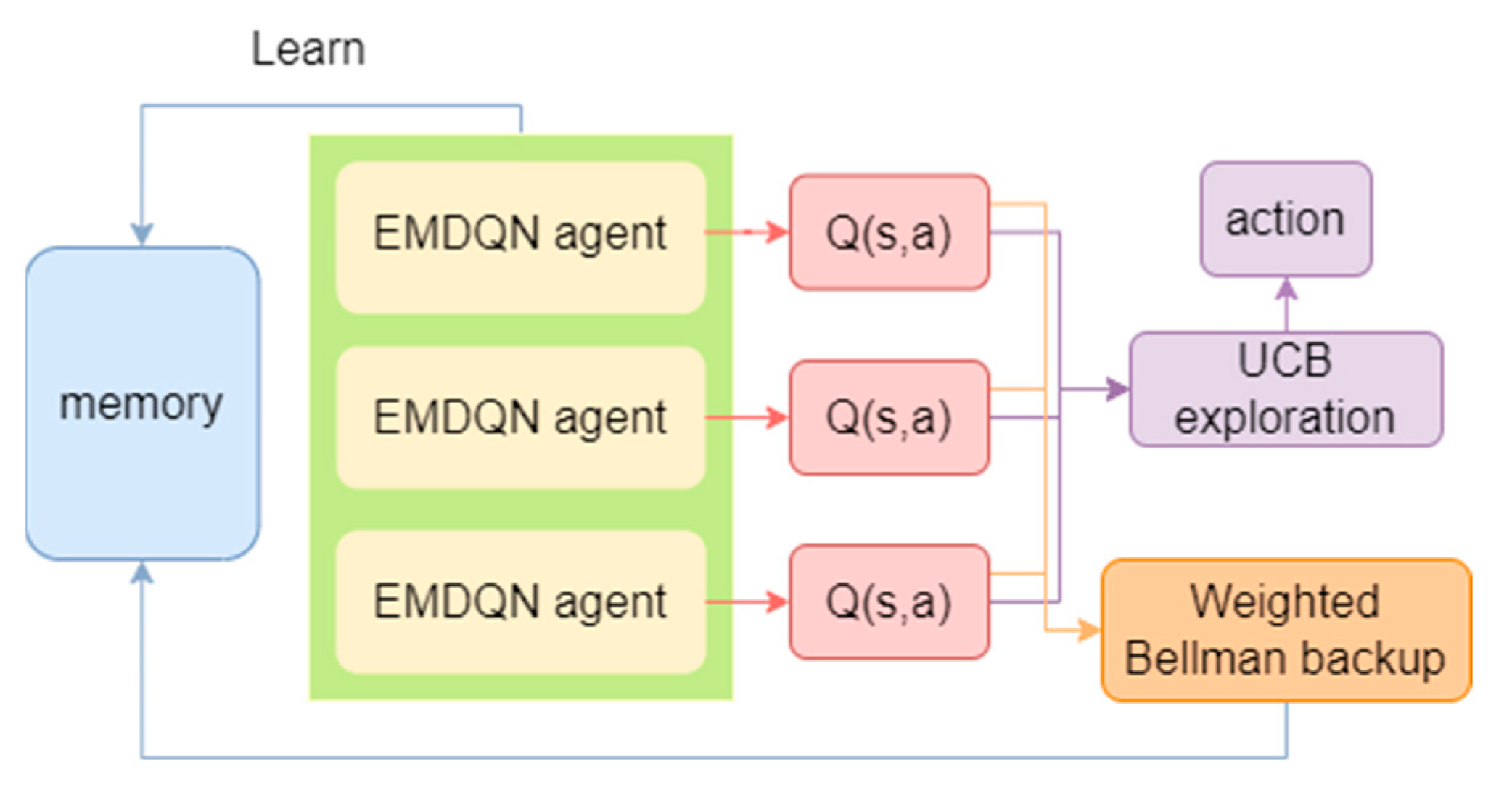
As shown in
Figure 3, ensemble learning is realized by a set of multiple EMDQN agents
, where
represents the parameter of the
-th agent. To diversify the training of the EMDQN agents, we randomly initialize the policy network of all EMDQN agents. In the training phase, we employ the
ϵ-greedy-based upper-confidence bound (UCB) exploration strategy [
34], as shown in Equation (24):
where
and
are the mean and standard deviation of the Q-values output by all MPNN policy networks
. The exploration reward
is a hyper-parameter. When
increases, the EMDQN agents become more active in accessing unknown state–action pairs.
The traditional DQN loss function (Equation (6)) may be affected by error propagation, that is, it propagates the target Q-network
error to the current state of the Q-network
. This error propagation can lead to an unstable convergence. To alleviate this problem, for each EMDQN agent
, this paper uses Bellman weighted backups, as shown in Equation (25):
where
represents the confidence weight of the set of target Q-networks in the interval [0.5, 1.0].
is calculated from Equation (26), where the weight parameter
is a hyper-parameter,
is a sigmoid function,
is the empirical standard deviation of all target Q-networks
.
reduces the weights of sample transitions with high variance between target Q-networks, resulting in better signal-to-noise ratios for network updates.
4.5. The Working Process of the EMDQN Agent
The working process of the EMDQN agent at each iteration is described in Algorithm 1. We first reset the environment and obtain the environment link capacity and traffic demand tuple
(line 1). Subsequently, we execute a loop to continuously assign traffic demands. In the process, we compute
shortest links (Line 3) and allocate the traffic demand for each shortest link through
cycles (Lines 4–8). Based on this, we can compute the Q-value for each action. We select actions using an
-greedy-based UCB exploration strategy (Line 9); subsequently, we apply the chosen route to the environment (Line 10). We store the rewards and state transfer during the interaction with the environment in the experience replay buffer (Line 11) while applying the transferred state (Line 12). The cycle stops when any link is unable to carry the traffic demand. Next, we execute the agent learning phase. For the sampled batch (Line 15), we plot the mask using the Bernoulli distribution (Line 16) and calculate the batch weight using all EMDQN agents. Following that, we multiply the sample by the weight and mask to minimize
(Line 18). Finally, we evaluate the set of EMDQN agents in the environment (Line 21) and collect the rewards, as well as the status of the environment, in the evaluation process to analyze the training situation of the EMDQN agent.
| Algorithm 1: working process of the EMDQN agent |
| 1: s, demand, src, dst ← env.reset() |
| 2: while (Done != False) do |
| 3: k_path ← compute_k_path(k, src, dst) |
| 4: for i ← 1 to k do |
| 5: path ← get_path(i, k_path) |
| 6: s’ ← allocate(s, path, src, dst, demand) |
| 7: k_Q[i] ← compute_Q(s’, path) |
| 8: end for |
| 9: a ← act(k_Q, ε, k_path, s) |
| 10: s’, r, done, demand’, src’, dst’ ← env.step(s, a) |
| 11: agent.rememble(s, a, r, s’, done) |
| 12: s, demand, src, dst ← s’, demand’, src’, dst’ |
| 13: end while |
| 14: for i ← 1 to STEP do |
| 15: batch ← sample() |
| 16: m ← bernoulli() |
| 17: for each agent i do |
| 18: Update agent by minimizing |
| 19: end for |
| 20: end for |
| 21: agent.evaluate() |
5. Experiments and Analysis
In this section, we simulate the SD-OTN routing scenario using the OpenAI gym framework to train and evaluate the EMDQN algorithm. Furthermore, we conduct experiments and analyses by adjusting the hyper-parameters and evaluating the algorithm load-balancing ability and generalization ability.
5.1. Experimental Environment
The computer used for the experiments has an AMD R5 5600G processor with a base frequency of 2900 MHz, a 2 TB solid-state drive, and 32 GB of RAM. The experiment uses the Tensorflow deep learning framework to implement the EMDQN algorithm. We select NSFNET, GEANT2, and GBN for the optical transmission network topology, with the lightpath bandwidth being 200 ODU0 bandwidth units, as shown in
Figure 4. Among these, the NSFNET network contains 14 ROADM nodes and 21 lightpaths, the GEANT2 network contains 24 ROADM nodes and 36 lightpaths, and the GBN network contains 17 ROADM nodes and 27 lightpaths.
In this paper, the lightpath bandwidth requirements are expressed as multiples of ODU0 signals, i.e., 8, 32, and 64 ODU0 bandwidth units. In each episode, the environment generates a traffic demand tuple at random. Additionally, the EMDQN agent should assign the appropriate route for each tuple received. If the assignment is successful, it will receive a reward as defined in Equation (1). Otherwise, it will not be rewarded. Since the new traffic demand is randomly generated, the routing policy designed by the EMDQN agent does not rely on traffic demand distribution information, reducing the EMDQN agent’s overfitting to the particular network scenario used for training.
5.2. Hyper-Parameters Settings
We experimentally select suitable hyper-parameters for the EMDQN agent, as shown in
Figure 5. In the experiments, we chose the NSFNET as the experimental network topology. The size of the link-hidden state is related to the amount of coding information. We set the size of the link-hidden state to twenty and the number of feature values to five, and filled the rest with zero. To facilitate observation, we smoothed the data when drawing the graph.
Figure 5a shows the training results for the different numbers of EMDQN agents. When the number of agents is high, the training slows down and aggravates the overfitting of DRL agents in the application scenario, resulting in poorer results. The performance is optimal when the number of EMDQN agents is two.
Figure 5b shows the training results of the stochastic gradient descent algorithm with different learning rates. When the learning rate was 0.001, the algorithm reward achieved the highest value.
Figure 5c shows the training results for different decay rates of
. In the initial stage of training,
is close to 1. We executed 70 iterations and started to reduce
exponentially using
-decay until it decreased to 0.05. During the process of
reduction, the training curve tends to flatten out, finally reaching convergence. The training results show that the reward value curve is most stable after convergence when
-decay is 0.995.
Figure 5d shows the training results for different
values in Equation (11).
denotes the exploration reward of the EMDQN agent. From the results in
Figure 5d, it is clear that the algorithm reward value is highest when
value is 5.
Figure 5e depicts the training results for different weight parameters
in Equation (14). In this paper, we set the size of samples to 32. As
increases, the sample weights converge and become less than one, which affects the sample efficiency of the EMDQN. The reward of this algorithm reaches its highest value when the value of
is 0.05.
Table 2 shows some relevant parameters of the EMDQN and values taken after tuning the parameters.
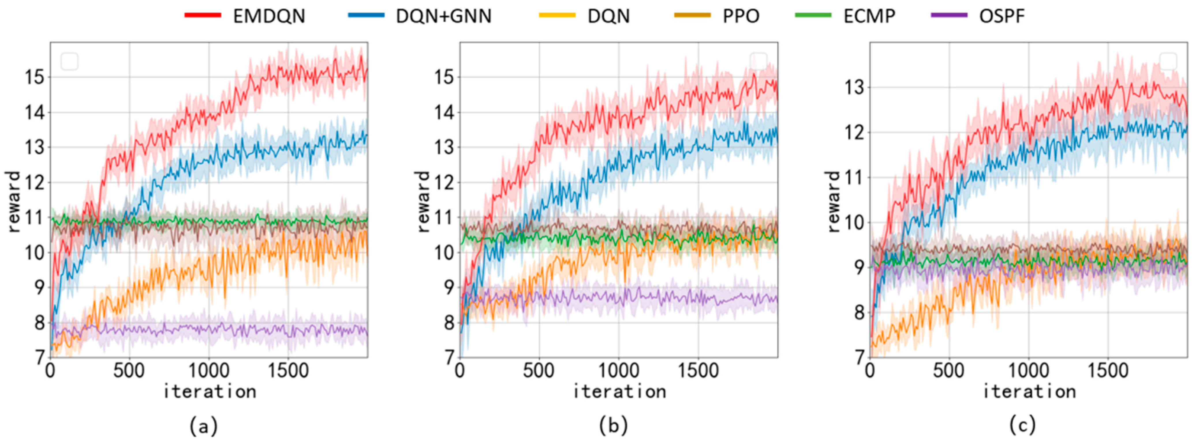
5.3. Load-Balancing Performance Evaluation
In this section, we experimentally evaluate the EMDQN in the three network topologies, as described in
Section 5.1. The DRL agent runs 2000 iterations. In each iteration, the agent trains 50 episodes and evaluates 40 episodes. Furthermore, the DRL agent updates the network during the training period. During the evaluation, the DRL agent does not update the network; rather, it applies the action to the environment intending to maximize the Q-function, and subsequently records network state data, such as rewards, link utilization, and throughput for each episode.
We implement other SDN solutions for performance comparison with EMDQN algorithms, such as OSPF [
7], ECMP [
8], DQN [
17], PPO [
19], and DQN+GNN [
26]. The DQN+GNN is an ablation experiment among the compared algorithms, i.e., a performance comparison of the EMDQN model with ensemble learning removed. The DQN and PPO are classic DRL algorithms that use a fully connected feedforward NN as a policy network. The OSPF is an open shortest path algorithm that performs an action selection by calculating the shortest number of hops of the link traversed between the source and destination nodes. The ECMP algorithm is an equal-value multipath routing protocol that allows the use of multiple links simultaneously in the network. The ECMP algorithm distributes the bandwidth demand equally over
lightpaths in this experiment. Furthermore, OUD0 signals are not divisible, but we can verify the performance in other network scenarios in this way.
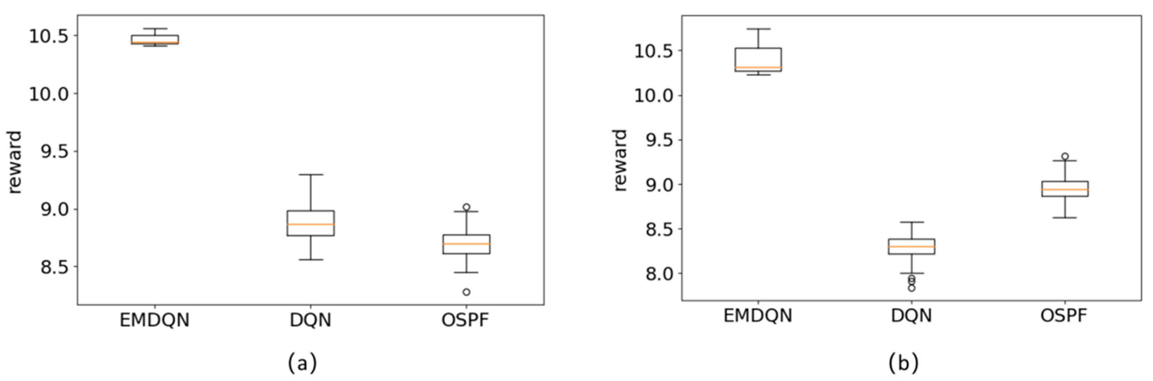
Figure 6 shows the average reward of all algorithms for the three evaluation scenarios, where the confidence interval is 95%. In this paper, we design the reward based on whether the bandwidth demand can be successfully allocated. The greater the reward, the more bandwidth demand is successfully allocated, and the better the network load-balancing capability. In all three evaluation scenarios, the EMDQN algorithm proposed in this paper performs better than other algorithms after convergence. The EMDQN algorithm outperforms the DQN+GNN algorithm with ensemble learning removed after convergence by more than 7%, demonstrating that the multi-agent ensemble learning approach can effectively improve the convergence performance of the DQN. Additionally, the EMDQN and DQN+GNN outperform the classical reinforcement learning algorithms (DQN and PPO) by more than 25% in all three evaluated scenarios. This indicates that the MPNN can effectively improve the decision performance of the reinforcement learning model by capturing information about the relationship between the demand on links and network topology. The DQN and PPO algorithms perform about as well as the ECMP algorithm after convergence. The OSPF algorithm, on the other hand, routes all flow requests singularly to the shortest path. Since this method is based on fixed forwarding rules, it can easily lead to link congestion. Therefore, the OSPF algorithm is only close to ECMP in the GBN scenario and the lowest in other scenarios.
Table 3 shows the average throughput of each algorithm in ODU0 bandwidth units for the three network topologies.
Table 4 displays the average link utilization of each algorithm across the three network topologies. The average throughput and link utilization of the EMDQN are higher than those of other algorithms under various network topologies, indicating that the EMDQN algorithm has a better load-balancing capability for the network after convergence. The performance of the EMDQN algorithm is higher than that of the DQN+GNN algorithm, which is a good indication that ensemble learning can improve the convergence performance of the model. The results show that the EMDQN has excellent decision-making abilities.


 ,
, 


